
Abstract
The LaSaXing Oilfield has entered the ultra-high water cut stage, and the original evaluation indexes of water flooding development effect cannot reflect development status of the oilfield. In order to correctly evaluate the water flooding development effect of the oilfield at ultra-high water cut stage, the indexes were extensively selected in terms of geological conditions, development technologies, production management, and economic benefits, and they were initially screened by observation principle, the Delphi method, and theoretical analysis. Then, the evaluation indexes were quantitatively selected by Pearson correlation analysis and combination of gray clustering-rough set to establish the index system evaluating water flooding development effect of oilfield at ultra-high water cut stage. The practice showed that the index system evaluating the development effect, which was scientific, objective, and strongly applicable, had great significance for comprehensive evaluation of the water flooding development effect of oilfield at ultra-high water cut stage, analysis of development potential, and formulation of development adjustment plan.
Introduction
The LaSaXing Oilfield in Daqing, the largest continental multilayer sandstone reservoir in China, is a representative of unitization sandstone oilfields at ultra-high water cut in China, and it is main part of the Daqing Oilfield with 85 % of gross reserve. After 50 years’ water flooding development, the LaSaXing Oilfield has entered the ultra-high water cut stage with sharply increased water–oil ratio and significant variation of oil–water distribution, development dynamic, and development law, and it faces the challenge of sharply rising water cut, serious production decline, seriously inefficient and ineffective circulation, and difficulty of tapping reservoir potential (Wei et al. 2013; Zhu et al. 2015). In order to maintain long-term stable production in the LaSaXing Oilfield, it is necessary to evaluate the water flooding development effect at ultra-high water cut stage, which has great significance for analyzing potential of oilfield and formulating the applicable development and adjustment program. The scientific evaluation index system is a prerequisite for evaluation of development effect at the ultra-high water cut stage, and the primary work is to screen and establish the evaluation index system (Liu and Xiao 2010).
The research on index system and methods evaluating water flooding development effect are variable worldwide. Since the 1950s, Guthrie and Gerenbegrer (1955), Wright (1958), Parts and Matthews (1959), and Arps (1956) from USA and Щeлкaчeв B (Tong 1981) from former Soviet Union have considered recoverable reserves and recovery factor, production decline rate as indexes evaluating rationality of developing oilfield through water injection. There is little research on the evaluation indexes and method of water flooding development outside China; especially, there is no report on the index system evaluating the water flooding development effect at the ultra-high water cut stage. Comparatively, there is more research on the evaluation indexes and method in China. However, most of methods are applicable in comparative evaluation of oilfield at middle-high water cut stage based on single indexes or multiple indexes and given criteria, and comprehensive evaluation by combining several indexes and applying fuzzy mathematical methods, which are one-sided and not applicable in development at ultra-high water cut stage (Huang and Tang 2000; Zhang et al. 2005; Zhang 2012; Liu et al. 2008; Tang et al. 2001; Jiang et al. 2008). There are few articles about evaluation index system of water flooding development effect at ultra-high water cut stage and its screening method. An evaluation index system applicable in ultra-high water cut stage and its selection method were presented by Yuan (2009) and Sun (2006), but its index system failed to cover the geological characteristic factors and was not capable of quantitatively evaluating some indexes. In addition, selection of indexes based on the statistical occurrence frequency quoted in the literatures is unreasonable because of strong subjective randomness and omission of indexes. The method of indexes selection presented by Ding (2009), Shi (2009), and Li et al. (2012) are strongly subjective and empirical, and their evaluation index system is lack of pertinence and practicality. The investigation shows that the index system of water flooding oilfield at ultra-high water cut stage has been not established worldwide, but it is a prerequisite for understanding and evaluating development rules and status of water flooding oilfield, and systematically and effectively determining the development effect. Therefore, effective selection of the simple and representative evaluation index system is needed to evaluate water flooding oilfield at ultra-high water cut stage. The indexes were extensively selected in terms of the geological conditions, development technologies, production management, and economic benefit, and they were initially selected by observation principle, the Delphi method, and theoretical analysis. Then, the evaluation indexes were quantitatively selected by Pearson correlation analysis and combination of gray clustering and rough set to establish the index system evaluating water flooding development effect of oilfield at ultra-high water cut stage, which provided a basis for quantitative and comprehensive evaluation of development effect.
Extensively selecting evaluation indexes of development effect at ultra-high water cut stage
The purpose of extensively selecting evaluation indexes of development effect is to reflect all information of development effect evaluation as well as possible and ensure that the evaluation indexes are not missed. According to the development characteristics of the LaSaXing Oilfield and through investigation of the literature, the outline of oilfield development management of PetroChina, Sinopec and CNOOC, and the oil and gas industry standards of the People’s Republic of China, and collection of the oilfield development experts experience, and field investigation, 94 indexes were extensively selected in terms of the geological conditions, development technologies, production management, and economic benefits which affect the development effect, and they are shown in Fig. 1.

Initial index set evaluating development effect of water flooding oilfield at ultra-high water cut stage
Indexes of geological conditions
In terms of the system theory, the index system of geological conditions is divided into reservoir physical property, liquid physical property, and reservoir integrity; index system of reservoir physical property is divided into reservoir geometric structure, reservoir characteristics, and reservoir sensitivity; index system of liquid property includes the properties of formation oil, water, and gas, such as oil viscosity and density; the index system of reservoir integrity includes the correlation between oil reservoir and liquid, and property indexes characterizing reservoir integrity. Specifically, the average reservoir pressure characterizes reservoir pressure system; the difference between reservoir pressure and saturation pressure characterizes oil energy in the reservoir; the geologic reserves characterizes reservoir capacity; the oil-bearing area characterizes the reservoir area; the average reservoir depth characterizes the average depth of the reservoir; the average reservoir temperature characterizes the reservoir temperature; the rhythmicity characterizes the sequence state of variation of macro reservoir permeability; the wettability characterizes the capability of oil and water preferentially wetting the surface of rock of oil reservoir; the connectivity coefficient characterizes the connectivity between reservoir pores; the permeability variation coefficient characterizes the macroscopic variation of permeability of sandbody; the permeability ratio characterizes the difference between maximum permeability and minimum permeability of oil-bearing sandbody.
Therefore, the index system of geological conditions of the reservoir at ultra-high water cut stage were established by collecting above analysis indexes, and 39 indexes in terms of geological conditions are shown in Fig. 1.
Indexes of development technologies
The indexes of development technologies, the dynamic technical variable reflecting the status of oil field development, are mainly applied to evaluate dynamic of development units and include perfection of well pattern, water injection condition, variation of water cut, oil production and liquid production, reserve–production condition, and exploitation degree. It is proved through years of development at ultra-high water cut stage in the Daqing Oilfield that the indexes of development technologies are the key to evaluating water flooding development effect at ultra-high water cut stage. Therefore, 35 indexes were refined further in seven aspects of development technologies, and each index of development technologies was reasonably quantified. The indexes are shown in Fig. 1.
-
1.
Perfection of well pattern is quantified by the reserves’ controlled degree of water flooding, the reserves producing degree of water flooding, the single-well-controlled geological reserves, the well pattern density, injector–producer ratio, injector–producer connection factor, etc.
-
2.
Water injection condition is quantified by three kinds of subindexes. The first is to reflect the utilization condition of water injection, including accumulative net injection percent, water flooding index, water consumption ratio and invalid water injection efficiency. The second is to reflect the maintenance of formation energy, including the formation pressure, the maintenance of formation pressure, and drawdown pressure. The third is to reflect the development condition of water injection, including cumulative injection–production ratio, annual injection–production ratio, and monthly injection–production ratio.
-
3.
Variation of water cut is quantified by water cut, water cut increasing rate, speed of water cut increase, water flooding condition, etc. The water flooding condition is not available in oilfield development data, so the recovery percent ratio is defined. The recovery percent ratio is the ratio between the ultimate recovery percent of reservoir (predicted or calculated by relation curve between water cut and recovery percent) and ultimate recovery factor calculated by relative permeability curve. The water flooding condition is determined with recovery percent ratio calculated through the relation curve between water cut and recovery percent of geological reserves.
-
4.
Variation of oil production is quantified by comprehensive decline rate, natural decline rate, oil recovery rate of geological reserves, dimensionless oil recovery rate, and productivity index, etc.
-
5.
Variation of liquid production is quantified by liquid productivity index and liquid recovery rate.
-
6.
Reserve–production condition is quantified by oil recovery rate of residual recoverable reserves, reserve–production ratio, reserve–production balance coefficient, etc.
-
7.
Exploitation degree is quantified by recovery factor, recovery percent of geological reserves, recovery percent of recoverable reserves, etc.
Indexes of production management
Indexes of production management are mainly applied to evaluate the effect of treatment and completion of workload, application of the oil–water well and surface equipment, and dynamic monitoring condition, and there are totally 12 indexes. The first is to quantify the development effect with initial oil production and initial water cut of new single well, gross treatment well times, effective rate of treatment, oil increment of single-well time of treatment, etc., which reflect effect of the workload and treatment. The second is to quantify the development effect with open rate of oil–water well, comprehensive production time efficiency of oil–water well, qualified ratio of zonal injection, etc., which reflect management status of oil–water well, as shown in Fig. 1.
Indexes of economic benefits
Economic benefit indexes are mainly applied to evaluate the economic benefits of management unit and include eight indexes, e.g., operation cost per ton of oil, internal rate of return, input–output ratio, as shown in Fig. 1. The calculation has big workload and great difficulty. The basic data for economic benefit indexes are from the economic evaluation parameter selection criteria (2008) and standard database of the Daqing Oilfield Co. (2014).
The indexes not only include qualitative indexes, but also indexes quantified by geological data of reservoir, development dynamic data, surface engineering, and economic data collected during development of oilfield. These indexes have correlation and similarity. The development effect is jointly influenced by some indexes and little influenced by other indexes. In order to consider influence of indexes on water flooding development effect at ultra-high water cut stage, four categories of indexes were combined to index set evaluating development effect of water flooding oilfield at ultra-high water cut stage. However, it is not necessary select all indexes as evaluation indexes, because they do not accurately and reasonably reflect the development effect at ultra-high water cut stage. In the past, the process of determining evaluation indexes of water flooding development effect was often subjective and empirical, and very few scholars screened the indexes based on scientific mathematical method, so the chosen indexes were often lack of pertinence and practicality. Thus, the correct and scientific methods are needed to select the indexes, and the principle of dynamics, independence, operability, representativeness, and objective should be considered when selecting and optimizing the index system.
Screening method of evaluation indexes of development effect
Observability principle
Observability principle is that the selected evaluation indexes have clear meaning and unified statistical caliber, and the index value is obtained with a statistical procedure. The indexes with fuzzy concept and not measurable actually, and those measurable theoretically but operated with difficulty should not be selected. Based on observability principle, the indexes evaluating development effect were initially screened, and those with data that cannot be obtained are eliminated, ensuring that the initially screened indexes meet the observability principle and can be quantified, and they could be applied. In this paper, 36 water flooding blocks in Sazhong, Sanan, Sabei, Xingbei, Xingnan, and Lamadian in the LaSaXing Oilfield were selected as evaluation objects; the original indexes inconformity with observation principle was removed through statistics. Therefore, 19 indexes, e.g., reservoir sedimentary facies, reservoir structure, reservoir sensitivity, components, and sulfur content of oil, critical temperature and pressure of gas, pH value, rhythmicity, wettability, connectivity coefficient, were removed, as shown in Fig. 2.

Diagram of removed indexes based on the observability principle
Delphi method
Considering the comprehensiveness of extensively selected indexes, numerous indexes in terms of geological conditions, development technologies, production management, and economic benefits were selected as evaluation indexes, and the screening had great difficulty because of complicated influence on the development effect at ultra-high water cut stage and relation between indexes. Thus, the indexes were further quantitatively screened with the Delphi method after screening them with the observability principle.
The Delphi method, also called as expert consultation method (Roberta and Andrea 2013), is essentially an anonymous feedback and consultation method. After collecting the expertise on the study issue, the expertise is organized and summarized, and anonymously fed back to experts. Then, the expertise is collected again, and it is organized and summarized next time until the consistent opinion is obtained. The method not only keeps the advantage of expert panels and brain storming, but also conquers the disadvantage of being interfered by mentality and stress of expert, and it is a scientific and practical method.
In order to obtain the rational and correct indexes screening results in national sci-tech major special project, the procedure of screening evaluation indexes of development effect at ultra-high water cut stage with Delphi method was determined through thorough design. (1) Establish the coordinating group. The group had four persons, including three professors and one lecturer. The main tasks were: preparation of the research topics, determination of the staffs, compilation of the expert questionnaire, organization of consultation, and statistics of data. (2) Choose experts. The experts have been engaged in oilfield development technologies and management in the LaSaXing Oilfield for 20 years, and they are familiar with characteristics of oilfield at ultra-high water cut stage and screening principles of evaluation indexes, e.g., dynamics, independence, operability, representativeness, and purposefulness. The experts have plentiful theoretical and practical experience, senior and professor-level senior technical professionals, master and doctor’s degree. They all have won science and technology awards in their fields. Considering the scale and the operational procedure of projects, 30 consultant experts were chosen in the project. (3) Make expert rating forms with evaluation indexes initially screened through observability principle. In the expert rating forms include the factors influencing evaluation indexes of development effect at ultra-high water cut stage, e.g., ranking scale, criterion, and familiarity. The quantization table is shown in Table 1. (4) Collect the expert rating forms for statistics and analysis, and calculate the statistical analysis result of expert ranking parameters of evaluation indexes. (5) Determine whether the second round of expert assessment is conducted based on the result of the first round of expert assessment. Return the calculation results and supplementary data of first round of expert assessment to the experts and let them re-evaluate the indexes to determine the new weight. (6) Analyze the result of second round of expert consultation to further screen evaluation indexes of development effect at ultra-high water cut stage.
On March 23–24, 2012, the expert consultation conference was held in the Daqing Oilfield, and 30 qualified experts were chosen for initial screening with the Delphi method. Two rounds of expert consultation were conducted to check and correct the data of consultation forms. The Excel database was established, and the statistical analysis was conducted with SPSS version 18.0. The main parameters of expert analysis of each index were calculated, and all main parameters meet the requirements, which showed that the initial screening based on the Delphi method was scientific and reasonable and provided basis for screening of indexes in next step. After initial screening with the Delphi method, 59 items of evaluation indexes were kept and 16 items of evaluation indexes were removed. The removed indexes are shown in Fig. 3.

Diagram of removed indexes based on the Delphi method
Theoretical analysis method
After screening through the Delphi method and combining with field production experience, the logical relationship between indexes influencing the development effect was divided into casual, equivalence, and process ones on basis of reservoir engineering theory (Jiang et al. 2008; Yuan 2009). Moreover, the indexes with casual, equivalence, and process relationship were eliminated by the theoretical analysis method, and the indexes related to each other were removed to further simplify the index system.
-
1.
The casual relationship is that one type of index is resulted from another type of index. The casual relationship is judged by the interactional mechanism and time sequence of occurrence. For example, the well pattern density and the producer–injector ratio are indexes with casual relationship with the reserves’ controlled degree of water flooding.
On basis of geological probability statistics, the formula calculating the reserves’ controlled degree of water flooding with probabilistic method is written as (Qi 1990):
$$\lambda = \frac{{\sum\nolimits_{i = 1}^{k} {\left( {\lambda_{i} \cdot N_{i} } \right)} }}{{\sum\nolimits_{i = 1}^{k} {N_{i} } }}$$(1)$$\lambda_{i} = 1 - \varepsilon^{{\frac{1}{2}}} \exp \left( { - \frac{{0.635A_{i} }}{{\psi (\varepsilon )d^{2} }}} \right)$$(2)$$\varepsilon = \frac{{N_{o} }}{{N_{w} }}$$(3)$$d = \sqrt {\frac{1}{f}}$$(4)where λ is the reserves’ controlled degree of water flooding; k is the gross of oil sandbody; λ i is the reserves’ controlled degree of water flooding of ith oil sandbody; N i is the oil geological reserves of ith oil sandbody, 104 t; A i is the oil-bearing area of ith oil sandbody, km2; d is the well spacing, m; ε is the producer–injector ratio, decimal; \(\psi (\varepsilon )\) is the correction factor of well pattern area (\(\psi (\varepsilon )\) = 0.866 for four-point well pattern, and \(\psi (\varepsilon )\) = 1 for five-point and nine-point well patterns); f is the well pattern density, well/km2; N o is the number of producers, well; N w is the number of injectors, well.
For example, in the northeast block of the Sazhong development zone, the oil-bearing area (A i ) of oil sandbody is 1.9 km2, the geological reserve is 369 million tons, and the block has experienced three well pattern thickenings. First infilling well density was 54.4 wells/km2, reserves’ controlled degree of water flooding was 83.2 %; the second infilling well density was 86.7 wells/km2, reserves’ controlled degree of water flooding was 93.1 %; in 2007, when the water cut of block was 92.5 %, the third infilling well pattern density was 134 wells/km2, reserves’ controlled degree of water flooding was 97.3 %. Five spot patterns, \(\psi (\varepsilon )\) = 1. So, the curve of influence of well pattern density and producer–injector ratio on reserves’ controlled degree of water flooding was calculated with formulae (2)–(4), which is shown in Fig. 4. The figure shows that the reserves’ controlled degree of water flooding is mainly influenced by well pattern density and producer–injector ratio, and it is outcome index of the well pattern density and the producer–injector ratio. The well pattern density and the producer–injector ratio are reason indexes and have causal relationship. At the ultra-high water cut stage, the development effect is improved a little by infilling wells and adjusting injector–producer ratio. Moreover, the influence of infilling well and adjusting injector–producer ratio on development effect is reflected by outcome index. Thus, through analysis of causal relationship, well pattern density and injector–producer ratio are eliminated.
Fig. 4 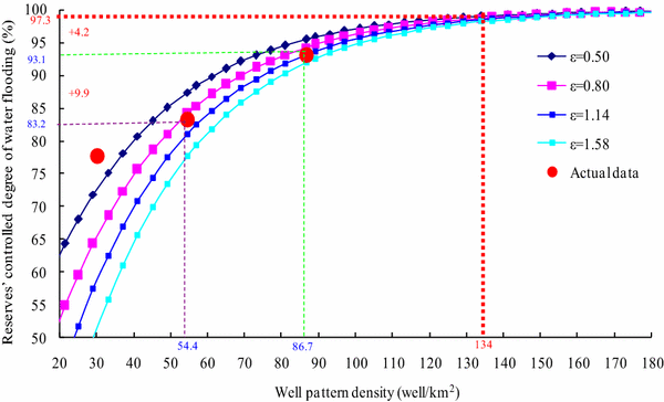
Relation curve between the well pattern density and injector–producer ratio and the reserves’ controlled degree of water flooding
-
2.
Equivalence relationship is that the indexes are not in the causal relationship chain, but have an equivalence relationship. It means that they are same type of indexes. For example, the well pattern density and the single-well-controlled geological reserves are equivalence relationship indexes. As is known, the recovery factor of water flooding oilfield is calculated with the Щeлкaчeв BH (1974) Formula, which is written as
$$E_{\text{R}} = E_{\text{D}} {\text{e}}^{ - af}$$(5)where E R is the recovery factor, %; E D is the oil displacement efficiency, %; a is the well pattern coefficient.
On basis of the Щeлкaчeв BH Formula, Yu (2001) replaced the well pattern density with the single-well-controlled geological reserves and presented another formula calculating the recovery factor of water flooding, which is written as
$$E_{\text{R}} = E_{{{\text{D}}1.0}} {\text{e}}^{ - BN/n}$$(6)where E D1.0 is the oil displacement efficiency with water cut of 1, %; B is the correction factor of well pattern; N is the geological reserve, 104 t; n is the well number, well.
With development data of the Sazhong development zone of the LaSaXing Oilfield, statistics and analysis of the good exponential relationship between the average single-well-controlled geological reserves and well pattern density (correlation coefficient) is conducted, and the formula is written as
$$N_{dj} = \frac{N}{n} = 29.65{\text{e}}^{ - 0.205f}$$(7)where N dj is the single-well-controlled geological reserves, 104 t.
It is shown in formulae (5) and (6) that the well pattern density is the most important factor influencing the recovery factor. With Formula (7), the well pattern density was transformed to the single-well-controlled geological reserves. During oilfield development, the well pattern density could be replaced with the single-well-controlled geological reserves under conditions of E D = E D1.0 and Formula (7), and they are equivalent to each other and have the coordinating relation. Thus, one of them is chosen to evaluate the development effect, and the well pattern is often chosen (Fig. 5).
Fig. 5 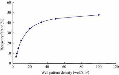
Curve of well pattern density and recovery factor in the Sazhong development zone of the LaSaXing Oilfield
Thus, based on analysis of equivalence relationship, the indexes, e.g., the single-well-controlled geological reserves, the oil increment of single-well time of treatment, and economic limit water cut of old wells, were eliminated.
-
3.
Process relationship is that the indexes are in the middle of the causal chain, and its influence on the result could be replaced with the previous reason indexes. For example, natural decline rate, water cut, water cut increasing rate, number of opening wells, formation pressure, and liquid productivity index have the process relationship, and they are process indexes. Based on the definition of decline rate, the formula of natural decline rate is written as (Tian et al. 2006):
$$D_{t} = 1 - \frac{{1 - f_{wt} }}{{1 - f_{wt - 1} }} \cdot \frac{{F_{t} }}{{F_{t - 1} }} \cdot \frac{{J_{lt} }}{{J_{lt - 1} }} \cdot \frac{{p_{rt} }}{{p_{rt - 1} }} \cdot \frac{{\left( {Ah_{\text{o}} \phi S_{\text{o}} \gamma_{\text{o}} /B_{\text{o}} } \right)_{t - 1} }}{{\left( {Ah_{\text{o}} \phi S_{\text{o}} \gamma_{\text{o}} /B_{\text{o}} } \right)_{t} }}$$(8)When the oilfield is in stable production, the liquid production is stable without stimulation treatment, namely F t = F t−1, J lt = J lt−1, p rt = p rt−1 and Formula (8) is simplified as (Tian et al. 2006):
$$D_{t} = \frac{{1 - f_{wt} }}{{1 - f_{wt - 1} }}V_{lt} B_{wt} = \frac{{f_{wt - 1} - f_{wt} }}{{1 - f_{wt - 1} }}$$(9)where f wt and f wt−1 are the water cut of tth and t − 1th year, %; F t and F t−1 are the well number of tth and t − 1th year, well; J lt and J lt−1 are the liquid productivity indexes of tth and t − 1th year, 104 t/MPa d; p rt and p rt−1 are the formation pressure of tth and t − 1th year; A is the oil-bearing area, km2; h o is the effective thickness, m; ϕ is the porosity, %; γ o is the oil density, g/cm3; B o is the oil volume factor, dimensionless.


It is shown in Formula (8) that the natural decline rate is product of the water cut, number of opening wells, formation pressure, and liquid productivity index. Thus, water cut, number of opening wells, formation pressure, and liquid productivity index are process indexes and could be replaced with the natural decline rate. Then, they are eliminated. Similarly, it is shown in Formula (9) and Fig. 6 that water cut and water cut increasing rate are process indexes and could be replaced with the natural decline rate. Thus, both of them were eliminated.

Curve of natural decline rate at different water cut in the Sazhong development zone of LaSaXing Oilfield
Through analysis of process relationship, water cut, water cut increasing rate, open rate of oil–water well, formation pressure, liquid productivity index, water consumption ratio, gross treatment well times, etc., are eliminated.
In conclusion, based on the theoretical analysis method, e.g., causal, equivalence, and process relationship, the indexes including geological reserves, oil-bearing area, well pattern density, injector–producer ratio, single-well-controlled geological reserves, water cut, water cut increasing rate, formation pressure, water flooding index, water consumption ratio, monthly injection–production ratio, gross decline rate, oil recovery rate of geological reserves, productivity index, liquid productivity index, liquid recovery rate, reserve–production ratio, recovery percent of geological reserves, gross treatment well times, oil increment of single-well time of treatment, open rate of oil–water well, production time efficiency of oil–water well, proportion of new casing damage well, economic limit water cut of old well are eliminated. 35 indexes were kept. The result of screening is shown in Table 2.
Data normalization prior to quantitative screening of indexes
Because of short sequence of statistical data and different dimensions of evaluation indexes, the original data should be normalized before quantitative screening to avoid calculation error resulted from different dimensions (Heffer et al. 1995).
-
1.
Normalization of the positive indexes
The positive index is the one that the greater the value, the better the evaluation result. The normalization formula is written as:
where x ik and u ik are the normalization value and the actual value of kth evaluation block of ith evaluation index, respectively; n is the number of evaluation blocks.
-
2.
Normalization of the negative indexes
The negative index is that the smaller the value, the better the evaluation result. The normalization formula is written as:
-
3.
Normalization of the interval indexes
The interval index reflects that the evaluation result is best when the index data are in a specific range. The normalization formula is written as:
where q 1 is the left boundary of the best interval of index data and q 2 is the right boundary of the best interval of index data.
It is expected to get higher value of quantitative indexes, e.g., geological reserves abundance, oil displacement efficiency, reserves’ controlled degree of water flooding, reserves producing degree of water flooding, recovery percent ratio, recovery percent of residual recoverable reserves, recovery factor, which are called as positive indexes; it is expected to get lower value of indexes, e.g., natural decline rate, comprehensive decline rate, water cut increasing rate, operation cost per ton of oil, which are called as negative indexes; it is expected to get value of a certain range of indexes, e.g., oil recovery rate of geological reserves, oil recovery rate of residual recoverable reserves, the maintenance of formation pressure, injection–production ratio, drawdown pressure, which are called as interval indexes. Above indexes have different dimensions and units, and evenly large difference of numerical order of value. Thus, the evaluation indexes should be normalized before being screened. Only indexes treated with scientific normalization can reflect real and comprehensive evaluation results.
Screening method of evaluation index based on Pearson correlation analysis
In order to further simplify the index system, first quantitative screening of the indexes was carried out through the Pearson correlation analysis. Pearson correlation analysis is that the evaluation indexes with bigger correlation are deleted through analysis of correlation between evaluation indexes of development effect to eliminate influence of repeated information of indexes on evaluation. Based on statistical principle, the formula of calculating the correlation coefficient r is written as (Hauke and Kossowski 2011):
where r ij is the correlation coefficient between the ith and the jth evaluation indexes; x ik is the normalization value for the kth evaluation block of the ith evaluation index; \(\overline{{x_{i} }}\) is the average value of the ith evaluation index.
The critical value M(0 < M < 1) is provided, when r ij > M, one of the evaluation indexes is deleted; when r ij < M, two evaluation indexes are kept. Through the Pearson correlation analysis, the index with the bigger correlation coefficient of same criterion is deleted, ensuring that the information reflected by the indexes is not repeated, and the index system is simple and effective.
Based on the above principles, with data of evaluation indexes of water flooding zones of the LaSaXing Oilfield, the Pearson correlation analysis of evaluation indexes is conducted using SPSS version 18.0 statistical software to obtain correlation coefficient matrix. The field experiences and practices in 36 blocks of the LaSaXing Oilfield show that when M = 0.7, the screened results is relative stable and reasonable; when M > 0.7, the selected results is not varied; when M < 0.7, the evaluation indexes increases, which is not consistent with reality and contradictory with the results of theoretical analysis. Thus, the indexes in Table 2 were screened through correlation analysis. Indexes including sandstone thickness, oil-bearing sandbody layers, accumulative injection–production ratio were removed, and 31 evaluation indexes were kept.
Principle and method of evaluation index screening based on gray clustering-rough set
Gray clustering analysis
After first quantitative screening through the Pearson correlation analysis, the non-operational and repeated indexes were removed to a large extent. However, the screening is conservative for comprehensiveness of results. So the gray clustering analysis of the screening results was needed, and one or more representative indexes were selected in each category to form evaluation index system, which not only met the requirements of comprehensiveness and independence, but also maximized the screening indexes of target.
It was assumed that there are m evaluation indexes, each one has n set of data, and the sequence is (Tan et al. 2003):
For i ≤ j, \(i,j = 1,2, \ldots ,m\), the gray absolute correlation degree X ij of X i and X j is written as:
Then, the correlation matrix between the indexes X i and X j is as follows:
where \(X_{ii} = 1,i = 1,2, \ldots ,m.\)
When critical value \(\lambda \in [0,1]\), the structure of gray correlation matrix A is not influenced by the value of A, and only the screening result of evaluation indexes is influenced. The practices in scientific, economic, and social fields show that λ > 0.5 is required, and when \(X_{\text{ij}} \ge \lambda\), x i and x j are of same type. During screening of the evaluation indexes, based on evaluation principle and F-statistics theory of development effect (Xie and Liu 2006), optimum critical value of λ is determined as λ = 0.7 with data of 36 zones of the LaSaXing Oilfield.
Each type of indexes reflects one aspect of development effect, so at least one index of each type should be included.
Rough set method
Rough set theory, proposed by Pawlak (1982) from Poland in 1982, is a mathematical theory and method dealing with uncertain, imprecise, and incomplete data, and has many advantages. Therefore, the index system was screened quantitatively with attribute reduction method of rough set (Pawlak and Skowron 2007, Ye et al. 2013, Xu et al. 2012).
Evaluation system S for water flooding development effect at ultra-high water cut stage is \(X = \left\{ {x_{1} ,x_{2} , \ldots ,x_{m} } \right\}\), each index has n sets of data. Then, the data of entire system is expressed with n × m matrix X.
Related definitions of rough set theory are:
-
1.
When \(u_{i} \ne u_{j}\), u i and u j are distinguishable in X.
-
2.
When u i in X is mutually distinguishable, then, S is distinguishable in X, denoted by ind(X).
-
3.
If x i in X is removed, S is still distinguishable and \({\text{ind}}(X - x_{i} ) = {\text{ind}}(X)\). Then, x i in X is reduced.
-
4.
If any index in X is not reduced, X is independent (any index in X is not indispensable in index system).
-
5.
For any subset \(A \subseteq X\) in X, when \({\text{ind}}(A) = {\text{ind}}(X)\) and A is independent, A is a minimal set in X: \({\text{MIN}}(X)\) (minimal set in X is not unique).
-
6.
The intersection X c of minimal subset in X is called as the kernel of X, \(X_{c} = \bigcap\limits_{i = 1}^{k} {\min_{i} (X)} ,k\) is number of minimal subsets.
The indexes in X are essential to describe the system, the solution to X c is generally based on discernable matrix, and the establishment of discernable matrix D is the key. For index system X of system S, the discernable matrix D is m rank matrix composed of subset of X:
The above definition showed that D is m rank matrix with zero main diagonal.
According to above method, the classification index data of gray clustering analysis were treated with standard discretization and the kernel was processed using MATLAB software, and the new index sets X c of each criteria layer were obtained. When the relation between x i and x j in X c is:
Or the correlation coefficient \(X(x_{i} ,x_{j} ) > \alpha\) (α is the threshold of evaluation system), an index is removed or one index is displaced with other index, further simplifying X c. Combining with gray clustering constraints of the indexes in each criterion, the core index system (I c) evaluating water flooding development effect at ultra-high water cut stage is determined.
Determination of evaluation index system of development effect
With the index screening method of combining qualitative and quantitative analysis, the indexes were selected step-by-step based on the building principle of evaluation index system of water flooding development effect at ultra-high water cut stage (Fig. 7). Eighteen main evaluation indexes of development effect were finally selected:

Diagram of principle of establishing evaluation index system of development effect of water flooding oilfield at ultra-high water cut stage
-
1.
Evaluation indexes reflecting geological conditions: channel sand ratio, effective thickness, effective permeability, variation coefficient of permeability, initial oil saturation, geological reserves abundance, oil displacement efficiency.
-
2.
Evaluation indexes reflecting development technologies: reserves’ controlled degree of water flooding, reserves producing degree of water flooding, maintenance of formation energy, cumulative net water injection, comprehensive decline rate, water cut increasing rate, oil recovery rate of residual recoverable reserves (reserve–production ratio), and water flooding condition (recovery percent ratio).
-
3.
Evaluation indexes reflecting production management: comprehensive production time efficiency of oil–water well, effective rate of treatment.
-
4.
Evaluation indexes reflecting economic benefit: operation cost per ton of oil.
According to the principle of mathematical statistics, the analysis and determination of rationality of evaluation index system with SPSS version 18.0 software showed that 19.1 % (18/94 = 19.1 %) of initial indexes reflected 97.4 % of original information, and the index system was proved to be reasonable. The application of evaluation indexes system in 36 development zones of the LaSaXing Oilfield in 2014 and 2015 showed that the selected indexes system accorded with the conditions of water flooding development oilfield at ultra-high water cut stage and reflected the water flooding development characteristics of the LaSaXing Oilfield. The investigation shows that there is no public report about evaluation indexes system and selection method applied in the Daqing Oilfield, other oilfields in China, and similar oilfields overseas.
Conclusions
-
1.
Eighteen indexes evaluating water flooding development effect of oilfield at ultra-high water cut stage in terms of geological conditions, development technologies, production management, and economic limit were screened through observation principle, the Delphi method, theoretical analysis, Pearson correlation analysis, and combination of gray clustering-rough set to establish the evaluation index system, and the index system was applied in the LaSaXing Oilfield of Daqing.
-
2.
Screening of evaluation indexes of water flooding development effect of oilfield at ultra-high water cut stage only relying on subjective method or objective statistics is not scientific. The indexes were screened by combining qualitative analysis and quantitative screening, which not only ensures that the screened indexes have the largest influence on evaluation result of criteria layer, but also avoids repetition of information of the same kind of index.
References
Arps JJ (1956) Estimation of primary oil reserves. Trans AIME 207:182–186
China’s National Development and Reform Commission (2008) SY/T 6511-2008 economic evaluating technical requirement for oil field development project and adjustment project. China’s National Development and Reform Commission
Щeлкaчeв BH (1974) Bлияниe нa Heфтeoтдaчy плoтнocти ceтки cквaжинииx paзмeшeния. нx 6:26–30
Daqing Oil Field Co. (2014) Criteria for selection of parameters of economic evaluation and interim measures. Daqing Oil Field Co., Daqing, pp 1–6
Ding QQ (2009) Study on the evaluation methods of development effects of waterflooding typical blocks in Lasaxing oilfield. Daqing Petroleum Institute, Daqing
Guthrie RK, Gerenbegrer MH (1955) The use of multiple correlation analysis for interpreting petroleum engineering data. In: Drilling and production practice. American Petroleum Institute, pp 130–137
Hauke J, Kossowski T (2011) Comparison of values of pearson’s and spearman’s correlation coefficients on the same sets of data. Quaest Geogr 30(2):87–93
Heffer KJ, Fox RJ, McGill CA (1995) Novel techniques show links between reservoir flow directionality, earth stress, fault structure and geomechanical changes in mature waterfloods. SPE J 2:91–98
Huang BG, Tang H (2000) Evaluation index system and evaluation method for waterflooding development effect. Southwest Petroleum Institute press, Nanchong, pp 16–25
Jiang RZ, Liu XB, Wang HJ et al (2008) Application of variables synthetical selection in the production evaluation for oilfelds in high water-cut period. Pet Geol Recovery Effic 15(2):99–101
Li B, Bi YB, Pan H et al (2012) Combination method for selecting comprehensive oilfield development effect evaluation targets. Pet Forum Sci Technol 3:38–41
Liu CL, Xiao W (2010) Index system of the water flooding development of oil fields and its structural analysis. Pet Explor Dev 37(3):344–348
Liu XT, Yang CD, Yang J et al (2008) A new discussion on comprehensive evaluation system of development effect in complex fault-block reservoirs. Fault Block Oil Gas Field 15(1):80–83
Parts M, Matthews CS (1959) Prediction of injection rate and production history for multifluid five-spot floods. JPT, May 98
Pawlak Z (1982) Rough sets. Int J Inf Comput Sci 11:341–356
Pawlak Z, Skowron A (2007) Rudiments of rough sets. Inf Sci 177(1):3–27
Qi YF (1990) Some theoretical considerations on optimal well pattern analysis in a water flooding sandy oil reservoir. Acta Pet Sin 11(4):51–60
Roberta T, Andrea F (2013) Standardising HSE training through Delphi. SPE 164939
Shi CF (2009) A stuty on methods of evaluating oil field development system of water flooding. Chinese Geology University, Beijing
Sun W (2006) Study of evaluation system and methods for oilfield development in high water-cut stage. University of Petroleum, Dongying
Tan HQ, Peng CC, Wu GH et al (2003) Gray clustering analysis and its application to petroleum exploration in Gudong area. Oil Gas Geol 3(1):97–101
Tang H, Li XX, Huang BG et al (2001) Using responding factors to evaluate comprehensively water flooding effect. J Southwest Pet Inst 23(6):38–40
Tian XD, Wang FL, Shi CF et al (2006) Variation law of production decline rate in Lasaxing oilfield. Acta Pet Sin 27(S):137–141
Tong XZ (1981) Oil well production and reservoir dynamic analysis. Petroleum Industry Press, Beijing, pp 37–60
Wei HT, Lin YB, Shi JP et al (2013) Study on the seepage law of oil-water during development of Changyuan Reservoir. J Southwest Pet Univ (Sci Technol Ed) 35(6):109–114
Wright FF (1958) Field results indicate significant advances in water flooding. JPT
Xie JJ, Liu CP (2006) Fuzzy mathematics method and its application. Huazhong University of Science and Technology Press, Wuhan, pp 2–5
Xu WH, Li Y, Liao XW (2012) Approaches to attribute reductions based on rough set and matrix computation in inconsistent ordered information systems original research article. Knowl-Based Syst 27(3):78–91
Ye DY, Chen ZJ, Ma SL (2013) A novel and better fitness evaluation for rough set based minimum attribute reduction problem. Inf Sci 222:413–423
Yu QT (2001) Determination of trend maximum well number and evaluation method for infilling efficiency. Pet Geol Oilfield Dev Daqing 20(4):22–25
Yuan BG (2009) Evaluation system of development effect in Ultra-high water cut stage of water flooded oilfield. Pet Geol Oilfield Dev Daqing 28(2):53–58
Zhang JF (2012) Evaluation methods of development effect for water drive oilfield and development trend. Lithol Reserv 24(3):118–122
Zhang XZ, Zhang LH, Xiong Y et al (2005) Evaluation method and its application in developing high water cut oilfield. Daqing Pet Geol Oilfield Dev Daqing 24(3):48–50
Zhu LH, Du QL, Jiang XY et al (2015) Characteristics and strategies of three major contradictions for continental facies multi-layered sandstone reservoir at ultra-high water cut stage. Acta Pet Sin 36(2):210–216
Acknowledgments
This paper is financially supported by the national sci-tech major special project of China (2011ZX05010-002 and 2011ZX05052-004), Key Project of Heilongjiang Education Apartment (12511z003), and Project of Daqing Oilfield Co., Ltd (DQYT-0505003-2014-JS-305, DQYT-0505003-2015-JS-220, and DQYT-0501002-2014-JS-83).
Author information
Authors and Affiliations
Corresponding author
Rights and permissions
Open Access This article is distributed under the terms of the Creative Commons Attribution 4.0 International License (http://creativecommons.org/licenses/by/4.0/), which permits unrestricted use, distribution, and reproduction in any medium, provided you give appropriate credit to the original author(s) and the source, provide a link to the Creative Commons license, and indicate if changes were made.
About this article

Cite this article
Wen, H., Sun, N. & Liu, Y. Index system evaluating water flooding development effect of oilfield at ultra-high water cut stage. J Petrol Explor Prod Technol 7, 111–123 (2017). https://doi.org/10.1007/s13202-016-0249-3
Received:
Accepted:
Published:
Issue Date:
DOI: https://doi.org/10.1007/s13202-016-0249-3