
Abstract
This paper investigates the dynamic angle of repose underneath the submarine pipeline. A series of tests are carried out to explore the bottom velocity in the scour hole for the case of with spoiler, and gap-ratio in unidirectional current. On that basis, the formulas of dynamic angle of repose in the scour hole are proposed using a sand deposition model. The formulas consider the bottom velocity (which is mainly influenced by the spoiler height and gap-ratio) that dominates the angle of repose. The calculation results are verified by the test data and a good agreement is obtained.
Introduction
As an important carrier, submarine pipeline was widely used to transport oil and gas from offshore to land. Nevertheless, due to the pipeline’s suspending caused by local sour, the slippage may exist and induce the accidents of pipe destruction. The extent of slippage is determined by the shape of scour hole. Related literature shows that the angle of repose is one of the main influencing factors for the profile of scour hole (Zhan and Xie 1996). Thus, the study of repose angle is significant for the pipeline maintenance and protection. By now, numerous related researches have been carried out to investigate this issue. Lane (1953) found that the angle of repose is proportional to the sediment diameter and varies with the sediment shape. Jin and Shi (1990) conducted physical model studies to explore the effect of the diameter and roughness of sediment on the angle of repose and obtained the formulas for different types of sediment. The formula of underwater repose angle was investigated by Shi et al. (2007) with a sand deposition model. Using a similar approach, Huang et al. (2008) derived the formulas of dynamic angle of repose for the cohesive and non-cohesive sediment. Yang et al. (2009) experimentally studied the angle of repose according to the conception of exposure degree. The repose angle for the submarine pipeline without spoiler was investigated by Yang et al. (2011). Nakashima et al. (2011) concluded, using the two-dimensional discrete element method (DEM), that the angle of repose is greatly influenced by the friction coefficient and rolling friction values, but the impact of elemental radius and gravity is very small. More related studies can be found in Zhou et al. 2002; Liu et al. 2005 and Wang et al. 2010.
Although much has been done on the topic of the repose angle, there is comparatively little research on the angle under the submarine pipeline. This paper investigates the formulas of dynamic repose angle in the scour hole for a pipe with spoiler and various gap-ratios. The gap-ratio (e) refers to the ratio of the gap height (S) beneath the pipe over pipe diameter (D).
Physical model experiments
Experimental set up
The laboratory experiments in this paper include two cases. For case one, the test was carried out in an annular flume which is 24.8 m long, 0.5 m wide and 0.6 m deep. Two pipes with the same diameter are laid and fixed in the flume, which are pipe A and pipe B, as seen in Fig. 1a. Part of the flume surrounding the pipe B was filled with sand to imitate seabed. The height of the sand bed was 0.15 m and the length was 5 m; pipe A was laid on a fixed bed which was at the same level as the sandy bed. The experimental arrangement is shown in Fig. 1a.

Experiment arrangement
For the case two, it was carried out in a current sink, which is 30 m long, 0.6 m wide and 1.0 m deep. The thickness of sand bed was 0.2 m and the length was 20 m. The experimental arrangement is shown in Fig. 1b.
Experiment parameters and procedure
In case one, the length of the pipe in the experiments is 0.5 m with the outer diameter being, respectively, 0.07 m, 0.09 m and 0.11 m. The experiment put L = 0.25D and 0.5D (D is the pipe diameter) two heights of spoilers which are made by the organic glass on the top of the pipe (see Fig. 1c). The water temperature was measured using a thermometer and kept at a constant of 16 °C, which had a kinematic viscosity of 1.118 × 10⁻⁶ m2/s. Water depth was kept at a constant of 0.4 m for all experiments. The inflow velocity (u0) on the height of the horizontal pipe axes was 0.24, 0.3 and 0.4 m/s, respectively. Before each test, the water level was adjusted to a required height. The mean diameter of sand used in all experiment was 0.56 mm and the porosity of the sand was n = 0.49. The gap-ratio was zero in this case.
In case two, the length of the tested pipe in experiments was 0.6 m with the outer diameter being 0.10 and 0.11 m, respectively. Four heights of spoilers which are L = 0.125D, 0.25D, 0.375D and 0.5D were used in the test. The gap between seabed and pipe is S = 0.3 and 0.5, respectively (S is the gap height). The inflow velocity (u0) on the height of the horizontal pipe axes was 0.24, 0.3 and 0.4 m/s, respectively. The same type of sand was used in this case. The experiment parameters are listed in Table 1. The experiments in group A are mainly used to investigate the influence of parameter on the repose angle as well as calibrate the derived formula. Group B are mainly used to determine the parameters of bottom velocities k (Run 13) and k′ (Run 14) (see below). The mechanical properties of spoiler investigated are shown in Table 2.
Measurements were mainly carried out on the movement bed. The incoming flow velocity upstream of the pipe and the bottom velocity in the scour hole were measured using an acoustic doppler velocimeter (ADV). Such flow measurements were used to investigate the variation of bottom velocity for different height of spoiler and gap. Furthermore, after the scour attained equilibrium, the section profiles of the scour hole were measured using a measuring pin with the minimum precision of 0.1 mm so as to obtain the angle of repose and verify the formulas.
Theoretical considerations
Previous research showed that the dynamic angle of repose can be investigated by the initial two accumulated layers of sand which is a ‘two layered sand model’(Huang et al. 2008). Using a similar approach, the forces acting on the sand particle were investigated by a sand deposition model (see Fig. 2). It is assumed that the width of the two layer model is d, d refers to the mean diameter of sand particles; and the length is nd (here n is the particle number of the bottom layer).

The sand deposition model (revised after Huang et al. 2008)
In equilibrium, there exist two angles, the angle α upstream which begins at point E; and the angle β downstream which starts at point F (as shown in Fig. 3). The sand particle in this study is non-cohesive, namely, no viscous force is considered, and it is assumed to be a sphere to simplify the sand model and calculation. The forces acting on the sand are uplift force (FL), submerged weight (WS), drag force (FD), lateral force (FE), and frictional resistance (Rf), as shown in Fig. 3.

The forces acting on the sand particle
The dynamic angle of repose upstream (α)
The forces acting on the sand deposition model at pointE are shown in Fig. 3. The individual forces are discussed as follows, respectively:
-
1.
Uplift force FL: The uplift force on a sand grain can be expressed as:
$$ F_{\text{L}} = C_{\text{L}} \frac{\pi }{4}d^{2} \gamma \frac{{u_{\text{b}}^{2} }}{2g}. $$(1) -
2.
Submerged weight WS: The submerged weight of sand particle can be written as:
$$ W_{\text{S}} = \frac{1}{6}\pi d^{3} (\gamma_{\text{s}} - \gamma ). $$(2) -
3.
Drag force FD: The drag force on a particle mainly depends on the bottom velocity, and it can be expressed as:
$$ F_{\text{D}} = C_{\text{D}} \left( {1 + \frac{\sqrt 2 }{2}} \right)d^{2} \gamma \frac{{u_{\text{b}}^{2} }}{2g}. $$(3) -
4.
Lateral force FE: The lateral force of sand particle can be written as:
$$ F_{\text{E}} = \frac{1}{2}\left( {1 + \frac{\sqrt 2 }{2}} \right)^{2} (\gamma_{\text{e}} - \gamma )d^{3}. $$(4) -
5.
Frictional resistance Rf: The frictional resistance can be represented by submerged weight and uplift force.
$$ R_{\text{f}} = \left[ {\left( {n + \frac{1}{2}} \right)W_{\text{s}} - nF_{\text{L}} } \right]f_{0}. $$(5)
At equilibrium, the sum of drag force and lateral force is equal to the frictional resistance in the x direction.
Substituting Eqs. (1)–(5) into Eq. (6), the following equation was obtained:
And the angle α can be written as:
where CL is the coefficient of uplift force; CD is the drag force coefficient; d is the mean particle size of sand; f0 is the friction coefficient; g is the gravitational acceleration; n is the total number of grains in the bottom layer; ub is the bottom velocity of water in scour hole; α is the dynamic angle of repose upstream; γ is the bulk density of water; γs is the bulk density of sand particles; γe is the saturated wet density of sand; CL can be chosen as a constant of 0.178 (Qian and Wan 1983), and CD could be taken as a constant of 0.45 for the turbulence condition (Shao and Wang 2005); f0 can be written as f0 = tanα; n can be determined as \( n = \frac{\sqrt 2 }{2\tan \alpha } + \frac{1}{2} \) (Huang et al. 2008).
The dynamic angle of repose downstream (β)
The sand deposition model at point F is similar to the point E, as seen in Fig. 3. It is assumed that the flow velocity in the scour hole remains unchanged, so the formulas of forces keep the same. However, the direction of frictional resistance and lateral force becomes opposite, thus, the force equation is expressed as follows:
Substituting all parameters into Eq. (9), then the formula of angle β is obtained:
Due to the boundary effect of the seabed, the directions of flow before and after the lowest point in the scour hole are along the seabed, which accelerate the bed scour and sediment transport. As such, the angles are slightly smaller than the theoretical value, so that the formulas Eqs. (8) and (10) must be revised by the calibration coefficient δ and η:
where δ and η are less than 1 and can be obtained from experimental data.
Experiment results and discussion
Experimental observations
The velocity at the lowest point of the scour hole was measured with ADV for different incoming flow. The results show that the ratio of bottom velocity (ub) and inflow velocity (u0 which is the incoming velocity at the horizontal axis of pipeline), decreases as the Reynolds number increases, as seen in Fig. 4. For the pipe with spoiler (e.g. L = 0.25D, e = 0), the velocity ratio is remarkably greater than the no spoiler one. However, for the pipe with the gap-ratio of 0.3 and L = 0.25D, the ratio is significantly reduced and even smaller than the no spoiler case.

Variations of bottom velocity for various scenarios with D = 0.11 m
The sandy bed scouring beneath the pipe with different spoiler heights and velocities were investigated. It can be seen that the scour depth increased significantly as the spoiler height and incoming flow velocity increased (see, Fig. 5); besides, the deepest point of the scour hole moved further downstream. This indicates that the spoiler and fluid velocity have influence on the repose angle. As shown in Fig. 5a, b, for the same pipe size, the angle of α increases with the increment of incoming velocity; the angle β, however, has a converse trend which decreases as the velocity increase. For the given laboratory condition (e.g. given incoming velocity), the angle β is significantly reduced as the spoiler height increases; however, the angle α increases slightly (see, Fig. 5b, d, f). In addition, it clearly demonstrates that the increase of spoiler height and flow velocity leads to more sand transport.

Experimental photos show the scour beneath the pipe for various cases with D = 0.09 m
Determination of coefficients
-
(a)
Bottom velocity
For the pipe without spoiler and gap, the bottom velocity ub is only related to the Reynolds number. By fitting analysis of the experiment data (Run 01–09 without spoiler), the fitted curve is shown in Fig. 6. Using the least square method, the relation can be expressed as:
$$ \frac{{u_{\text{b}} }}{{u_{0} }} = - 0.0435[\lg (Re)]^{2} + 0.335\lg (Re) - 0.32 $$(13)where Re is the flow Reynolds number defined as Re = u0D/ν.
Fig. 6 
The fitting curve between ub/u0 and lg(Re)
-
(b)
The coefficient of k
When a spoiler is fixed on the pipe, the bottom velocity \( u_{\text{b}}^{\prime } \) is now related to the height of spoiler and the Reynolds number. Assuming that \( u_{\text{b}}^{\prime } \) can be expressed by ub with a correction coefficient k, which may be written as \( k = \frac{{u_{\text{b}}^{\prime } }}{{u_{\text{b}} }} = f\left( \frac{L}{D} \right). \) Figure 7 provides test data for Run 13, it can be seen that a linear relationship exists between k and L/D, also with the least square method, it can be expressed as:
$$ k = 0.37\left( \frac{L}{D} \right) + 1. $$(14)Fig. 7 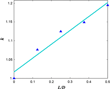
The relationship curve between k and L/D
-
(c)
The coefficient of k′
When the spoiler and gap both exist, the bottom velocity is related to the gap-ratio, spoiler height and the Reynolds number. Assuming \( u_{\text{b}}^{\prime \prime } \) now can be expressed by \( u_{\text{b}}^{\prime } \) with a coefficient of k′, namely, \( k^{\prime } = \frac{{u_{\text{b}}^{\prime \prime } }}{{u_{\text{b}}^{\prime } }} = f(e). \) For Run 14, the relationship between k′ and e is plotted in Fig. 8, the numerical relationship can be obtained by the method of least square:
$$ k^{\prime } = 0.25e^{2} - 0.49e + 1. $$(15)Fig. 8 
The relationship curve between k′ and e


Comparison of dynamic angle of repose between test values and calculated values
After comparing with the test data, it is found that when δ = 0.45 and η = 0.6 the test data fit the calculated values very well. The comparison between the calculated results [which is obtained by Eqs. (11) and (12)] and the experimental data for different conditions are discussed as follows:
-
1.
The pipe with spoiler but without gap
For a pipe with a spoiler installed on the top, Fig. 9 illustrates the relationship between angle of repose and sand Reynolds number. The sand Reynolds number is defined as Re * = u * d/ν (where u * is friction velocity). As seen in Fig. 9, for a certain pipe size, the angle α increases slightly as the sand Reynolds number increase; and there is a corresponding reduction for the angle β. This trend will be more marked, when the spoiler is higher. For a given incoming velocity, the angle α reduces slightly with the increase of pipe diameter; but there is a small increase for the angle β.
Fig. 9 
Comparison of calculated values and test data (radian value), the hollow symbols stand for α; the solid symbols stand for β; filled circleL = 0.25D calculated values: left pointing triangleD = 7 cm test, filled triangleD = 9 cm test, filled squareD = 11 cm test. Open star L = 0.50D calculated values: right pointing triangleD = 7 cm test, filled diamondD = 9 cm test, filled inverted triangleD = 11 cm test
For a small spoiler height (e.g. L = 0.25D), the values of angle α are within 0.35–0.47 and the angle of β are within 0.11–0.27. While the spoiler height is 0.5D, the values of α are within 0.36–0.49, and of β are within 0.06–0.26 (as shown in Table 3, Run 01–09). This indicates that the spoiler has a more obvious impact on the angle β than α. Besides, Fig. 9 shows a favorable match between the calculated results and measured data.
Table 3 The calculated value and test data for angle α and β -
2.
The pipe with spoiler and gap
Figure 10 shows the data for the existence of both spoiler and gap. It can be seen from Fig. 10 that there is a little reduction for angle α compared with the case of no gap; meanwhile, there is a noticeable increase for angle β (as shown in Table 3, Run 07–12). And this trend will become more obviously if the gap-ratio increases. As shown in Fig. 10, the angle α for e = 0.5 is a slightly smaller than that for e = 0.3 but a contrary trend exists for β. Also, reasonably good agreement between the calculated and experimentally measured angle is obtained.
Fig. 10 
Comparison of calculating values and test data (L = 0.25D), the hollow symbols stand for α; the solid symbols stand for β; filled circlee = 0.3 calculated values: filled squareD = 11 cm test values; open stare = 0.5 calculated values: filled inverted triangleD = 11 cm test values


Conclusion
This paper investigated the variations of bottom velocity and the dynamic angle of repose under various pipe sizes, spoiler heights, and gap-ratios. Based on the results presented above, the following conclusions can be drawn:
-
1.
The bottom velocity in the deepest point of scour hole without and with the spoiler and gap was discussed by experimental study. It increases with the increment of the Reynolds number and spoiler height but decreases with the gap-ratio. This indicates that spoiler enhances the seabed scouring but gap reduces the scouring.
-
2.
Using a sand deposition model, the formulas of dynamic angle of repose [e.g., Eqs.(11), (12)] for different conditions were obtained. The angle α increases with the growth of sand Reynolds number and spoiler height, but reduces as the gap-ratio. The angle β has a contrary trend.
-
3.
Comparison between the calculated values and experimental data shows that the formulas in this study can represent the variations of the angle of repose.
Inadequate and prospect
Our results may not be used to calculate the angle in the case of high Reynolds number, cohesive sediment and irregular sediment, however, it lays a theoretical foundation for further study on the dynamics angle of repose below the submarine pipeline.
Abbreviations
- C L :
-
The coefficient of uplift force, which is 0.178 (Qian and Wan 1983)
- C D :
-
The drag force coefficient, which is 0.45 (Shao and Wang 2005)
- D :
-
The diameter of the pipe
- D :
-
The mean particle size of sand
- e :
-
The gap-ratio (e = S/D)
- f 0 :
-
The friction coefficient
- g :
-
The gravitational acceleration
- k :
-
A correction coefficient
- k′:
-
A correction coefficient
- L :
-
The height of spoiler
- N :
-
The total number of grains in the bottom layer
- Re :
-
The flow Reynolds number
- Re * :
-
The Reynolds number of sand particle
- S :
-
The gap height
- u 0 :
-
The incoming velocity of water in upstream
- u b :
-
The bottom velocity of water on the seabed
- α :
-
The dynamic angle of repose upstream
- β :
-
The dynamic angle of repose downstream
- δ :
-
The calibration coefficient
- η :
-
The calibration coefficient
- γ :
-
The bulk density of water
- γ s :
-
The bulk density of sand particles
- γ e :
-
The saturated wet density of sand
References
Huang CW, Zhan YZ, Lu JY (2008) The formula of dynamic angle of repose for cohesive and non-cohesive uniform sediment. Guangdong Water Resour Hydropower 6:1–4
Jin LH, Shi XQ (1990) Study on the underwater angle of repose for model sand. J Sediment Res 3:87–93
Lane EW (1953) Progress report on studies on the design of stable channels by the bureau of reclamation. Proc ASCE 79(280)
Liu XY, Specht E, Mellmann J (2005) Experimental study of the lower and upper angle of repose of granular materials in rotating drums. Powder Technol 154:125–131
Nakashima H, Shioji Y, Kobayashi T, Aoki S, Shimizu H, Miyasaka J, Ohdoi K (2011) Determining the angle of repose of sand under low-gravity conditions using discrete element method. J Terrramech 48:17–26
Qian N, Wan ZH (1983) Sediment transport dynamics. Science Press, Beijing
Shao XJ, Wang XK (2005) Introduction to river dynamics. Tsinghua University Press, Beijing, p 38
Shi YL, Lu JY, Zhan Z, Huang CW, Yu JY (2007) The calculation of underwater angle of repose and dry density of sediment. Eng J Wuhan Univ 40(3):14–17
Wang W, Zhang JS, Yang S, Zhang H, Yang HR, Yue GX (2010) Experimental study on the angle of repose of pulverized coal. Particuology 8:482–485
Yang FG, Liu XN, Yang KJ, Cao SY (2009) Study on the angle of repose of nonuniform sediment. J Hydrodyn 21(5):685–691
Yang LP, Shi B, Guo YK (2011) Calculation on dynamic angle of repose for submarine pipeline on sandy Seabed. Appl Mech Mater 137:210–214
Zhan YZ, Xie BL (1996) Under water angle of rest for non-cohesive sediment. Int J Hydroelectr Energy 14(1):56–59
Zhou YC, Xu BH, Yu AB, Zulli P (2002) An experimental and numerical study of the angle of repose of coarse spheres. Powder Technol 125:45–54
Acknowledgments
This study was financially supported by the National High-Tech Research and Development program of China (863 Program, Grant No. 2008AA09Z309), National Nature Science Fund of China (Grant No. 50879084, 51279189), China Scholarship Council and University of Aberdeen.
Author information
Authors and Affiliations
Corresponding author
Rights and permissions
Open Access This article is distributed under the terms of the Creative Commons Attribution 2.0 International License (https://creativecommons.org/licenses/by/2.0), which permits unrestricted use, distribution, and reproduction in any medium, provided the original work is properly cited.
About this article
Cite this article
Yang, L., Shi, B. & Guo, Y. Study on dynamic angle of repose for submarine pipeline with spoiler on sandy seabed. J Petrol Explor Prod Technol 2, 229–236 (2012). https://doi.org/10.1007/s13202-012-0037-7
Received:
Accepted:
Published:
Issue Date:
DOI: https://doi.org/10.1007/s13202-012-0037-7