
Abstract
Firstly, based on the river health evaluation theory and starting from the integrity of the river system, the river health evaluation index system is selected. Secondly, the index systems of river health assessment including river morphology, hydrological and environmental characteristics, habitat elements and human activity characteristics are determined. Thirdly, set-pair (SPA) evaluation theory and extension were dealt with, a set-pair analysis-extension coupling model is constructed. Finally, taking Huangchuan Rive as an example, the ecological health evaluation on the river channel is carried out by using set-pair analysis-extension coupling model. The results of the comprehensive evaluation using the set-pair analysis-extension coupling method is obtained through calculation. It is proved by practice that the method of river health evaluation using the coupling model of set-pair analysis and extension theory could make full use of the data transformation and extension calculation, which shows the superiority in calculating correlation degree, and could reflect the determination and uncertainty of practical problems. It is possible to comprehensively consider all relevant factors. The paper provides a new idea for solving the relevant problems and obtains more accurate conclusion.
Introduction
River ecological health is an important aspect of river system management. With the development of industrial and agricultural production and social economy, river health has been paid more and more attention by all levels of society and governments (Meyer 1997: Gibson et al. 2016). With the understanding of the river natural attributes and water shortage challenges, the goal of river management has been evolved from a single water resources function to the multiple objectives of river ecosystem management (Thorpjh et al. 2006; Razmkhah et al. 2010). Accordingly, as an assessment tool and technical means, the contents of river health assessment are gradually changed to the integrity and sustainability of river ecosystem in long-term evolution under the dual action of natural and human activities(Zhang et al. 2010; Wei et al. 2019). A river health status should be a decision basis for regional development planning and river managers (Lee et al. 2010; OMID et al. 2014). Because the river health and life involve many factors including natural and social attributes, it has the characteristics of diversity, variability and uncertainty, therefore, the river ecological health evaluation system belongs to the typical complex system (Wei et al. 2019; Yang et al. 2016). Although the previous methods, such as variable fuzzy evaluation, gray theory, extension and set-pair analysis, have made beneficial progress, there still exist some defectives (Zhai et al. 2016; Ladon et al. 1999). For example, extension theory can take all factors into account comprehensively, but the correlation degree is often calculated with the interval important points, and consider those points as the best scheme, which could miss some important constraints and result in differences between the results and actual situations (Gao et al. 2017; Gao et al. 2007). The set pair analysis method could solve the intermediate transformation problems, but it is difficult to determine the coefficient of difference in the evaluation(Yang et al. 2015; Zhang et al. 2014). The combination of set-pair analysis with extension theory could not only apply extension theory to calculate correlation degree, but also reflect the determination and uncertainty of practical problems, therefore, the accuracy of river health evaluation should be improved. By using this method, the grade of samples to be tested could be reasonably assessed. Therefore, based on the construction of comprehensive evaluation index system of river health, this paper systematically studies SPA evaluation theory, extension theory and set-pair analysis-extension coupling method. The improved set-pair analysis method and extension theory are introduced. The set pair analysis and identical inverse partition method are applied to extensional set domain(Ellmore et al. 2015; Erst et al. 2012). A set-pair analysis-extension coupled comprehensive evaluation model for river health evaluation is constructed. A new perspective to evaluate river health is explored. Finally, taking the Huangchuan River (which is a main tributary of the Huaihe River) as an example, the ecological health evaluation is carried out by using the studied methods. The results of comprehensive evaluation using set-pair analysis-extension coupling method were obtained. It is proved from the results that the evaluation results have an important reference value for the water resources rational exploitation, the improvement of water efficiency and ecological environment.
Methods
Construction of river health comprehensive evaluation standard index system.
The comprehensive evaluation index system for river health is constructed according to the following five principles (Chen et al. 2014;Whited et al. 2012); (1) to form a comprehensive and relatively independent indicator system;(2) easy operation, easy access to evaluation data and information; (3) qualitatively reflect the degree of river health; (4) quantitative calculation; (5) real description of the river status. Based on those consideration, through literature investigation, field investigation, expert interview, combined with the characteristics of ecological environment and social-economic characteristics in river basin, the standard index system of river health evaluation was finally determined, which includes the characteristics of river morphology, hydrology, environment, habitat elements and human activities, see Table1.
Improved set-pair analysis based on extension theory
-
(1)
SPA evaluation theory
Set pair analysis was proposed by Zhao Keqin in 1989(Zhao 2000), which is based on the idea that divides the system's certainty into two aspects:" concordant "and" opposite". Uncertainty could be defined by the "difference". The concordant, opposite and difference (three aspects) are interconnected, influenced and transformed mutually(Wohle 2017; Xia and Yan 2004).Here,we introduce the correlation degree to express the uncertainty of the system, to quantify and identify the uncertainty.
Let set pair H = (A,B) is composed of set A and B. The set pair H could be separated to obtain N characteristics, in which, A and B share the opposite number of characteristics S、P, the remaining characteristics are F, which can be expressed using the following formula(1)
$$\mu_{AB} = \frac{S}{N} + \frac{F}{N}i + \frac{P}{N}j = a + bi + cj$$(1)In which, μAB is correlation degree; i is difference uncertainty coefficient; i ∈ (-1, 1); j is opposite degree coefficient; a、b、c is the concordant degree coefficient, difference degree and opposite degree coefficient under a certain characteristic respectively, which satisfies the condition a + b + c = 1.
Such kind of method can only make a rough analysis on the membership grade according to the a,b,c. It neglects the degree of comprehensive membership, and also ignores the importance of indicators and the coefficient of difference.
-
(2)
Theory of extenics
Born in 1983, Extenics is a new subject overlapped by mathematics, engineering sciences and philosophy(Liu. 2015). The extension theory takes physical element as the logical cell, and takes physical element theory and set-extension theory as the basis(Mingwu, Juliang, 2014). The physical element takes the ordered three dimension R = (thing, characteristic, quantity) = (N,C,V) as the basic elements to describe an event. Different objects can be represented by the elements with the same feature. Physical elements are extensible. Correlation degree k(x0) is the degree which an element belongs to an evaluation level, which can be calculated with the following Eq. (2).
$$k(x_{0} ) = \frac{{\rho (x_{0} ,X_{0} )}}{{\rho (x_{0} ,X) - \rho (x_{0} ,X_{0} )}}{\kern 1pt} {\kern 1pt} {\kern 1pt} {\kern 1pt} {\kern 1pt} {\kern 1pt} {\kern 1pt} {\kern 1pt} {\kern 1pt} {\kern 1pt} {\kern 1pt} {\kern 1pt} {\kern 1pt} {\kern 1pt} {\kern 1pt} {\kern 1pt} {\kern 1pt} {\kern 1pt} {\kern 1pt} {\kern 1pt} {\kern 1pt} {\kern 1pt} {\kern 1pt} {\kern 1pt} {\kern 1pt} {\kern 1pt} {\kern 1pt} {\kern 1pt} {\kern 1pt} {\kern 1pt} {\kern 1pt} {\kern 1pt} {\kern 1pt} {\kern 1pt} {\kern 1pt} {\kern 1pt} {\kern 1pt} {\kern 1pt} {\kern 1pt} \rho (x_{0} ,X) \ne \rho (x_{0} ,X_{0} )$$(2)$$\rho (x_{0} ,X_{0} ) = \left| {x_{0} - \frac{a + b}{2}} \right| - \frac{b - a}{2}$$$$\rho (x_{0} ,X) = \left| {x_{0} - \frac{c + d}{2}} \right| - \frac{d - c}{2}$$In which, ρ (x0, X) and ρ (x0, X0) are physical moment of point x0 to domain X and X0, respectively (Fig. 1), (x0, X)–(x0, X0) is the location of the point x0 to the relevant two domains.
Fig. 1 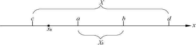
Schematic diagram of extension set theory domain

Improved set pair analysis–extension coupling method
-
(1)
The basic principle and evaluation steps
The flow chart of improved set pair analysis and extension coupling method is shown in Fig. 2
Fig. 2 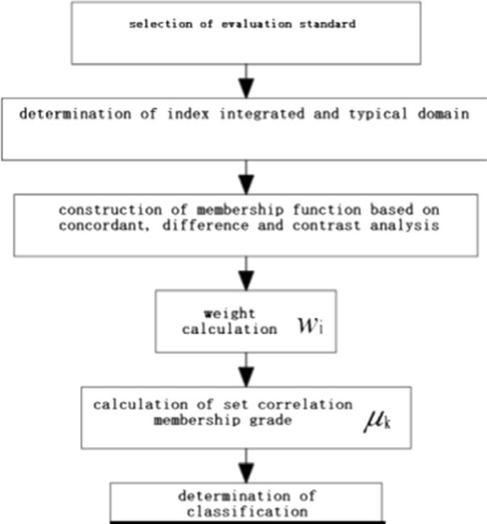
Flow chart of evaluation process in improved coupling set pair analysis and extension theory
-
(2)
Model construction
For an evaluation problem, let N = N1, N2, …, Nk, …, NK (k = 1,2, …, K) be entire domain, Cj is the jth (j = 1,2, …, m)evaluated indicator, vjk represents quantitative value of element Nk relevant to indicator Cj, then, the evaluated value for indicator k could be defined as the concordant Rk by using physical element. i,e.
$$R_{k} = (N_{k} ,C_{j} ,V_{k} ) = \left[ {\begin{array}{*{20}c} {N_{k} } & {C_{1} } & {V_{1k} } \\ {} & {C_{2} } & {V_{2k} } \\ {} & \vdots & \vdots \\ {} & {C_{m} } & {V_{mk} } \\ \end{array} } \right]$$(3)in which, Vk = (ajk, bj) is the value domain of Nk relevant to indicator Ci, then, the entire domain Rk is composed of the concordant elements from evaluated indicators, i.e.
$$\begin{gathered} \hfill \\ R_{K} = \left[ {\begin{array}{*{20}c} N & {N_{1} } \\ C & {V_{1} } \\ \end{array} {\kern 1pt} {\kern 1pt} {\kern 1pt} {\kern 1pt} {\kern 1pt} {\kern 1pt} {\kern 1pt} {\kern 1pt} {\kern 1pt} {\kern 1pt} {\kern 1pt} \begin{array}{*{20}c} {N{}_{2}} & {...} \\ {V_{2} } & {...} \\ \end{array} {\kern 1pt} {\kern 1pt} {\kern 1pt} {\kern 1pt} {\kern 1pt} {\kern 1pt} {\kern 1pt} {\kern 1pt} {\kern 1pt} \begin{array}{*{20}c} {N_{K} } \\ {V_{K} } \\ \end{array} } \right] = \left[ {\begin{array}{*{20}c} N & {C_{m} } & {N_{2} } & {...} & {N_{K} } \\ {C_{1} } & {(a_{11} ,b_{11} )} & {(a_{12} ,b_{12} )} & {...} & {(a_{1K} ,b_{1K} )} \\ {C_{2} } & {(a_{21} ,b_{21} )} & {(a_{22} ,b_{22} )} & {...} & {(a_{2K} ,b_{2K} )} \\ \vdots & \vdots & \vdots & \ddots & \vdots \\ {C_{m} } & {(a_{m1} ,b_{m1} )} & {(a_{m2} ,b_{m2} )} & {...} & {(a_{mK} ,b_{mK} )} \\ \end{array} } \right] \hfill \\ \end{gathered}$$(4)The section domain of the relevant evaluation indicators can be defined as;
$$R_{m} = \left[ {\begin{array}{*{20}c} N & {C_{1} } & {V_{1d} } \\ \begin{gathered} \hfill \\ \hfill \\ \end{gathered} & \begin{gathered} C_{2} \hfill \\ \vdots \hfill \\ \end{gathered} & \begin{gathered} V_{2d} \hfill \\ \vdots \hfill \\ \end{gathered} \\ {} & {C_{m} } & {V_{md} } \\ \end{array} } \right] = \left[ {\begin{array}{*{20}c} N & {C_{1} } & {\left\langle {a_{1d} ,b_{1d} } \right\rangle } \\ \begin{gathered} \hfill \\ \hfill \\ \end{gathered} & \begin{gathered} C_{2} \hfill \\ \vdots \hfill \\ \end{gathered} & \begin{gathered} \left\langle {a_{2d} ,b_{2d} } \right\rangle \hfill \\ \vdots \hfill \\ \end{gathered} \\ {} & {C_{m} } & {\left\langle {a_{md} ,b_{md} } \right\rangle } \\ \end{array} } \right]$$(5)in which, N represents the total grades of evaluation subjects, (amd, bmd) represents the value domain of indicator Cm under certain conditions. Then, Rp (p = 1,2, …, P) (the concordant physical elements relevant to total evaluation samples) is as follows;
$$R_{P} = \left\lfloor {\begin{array}{*{20}c} P & {p_{1} } & {p_{2} } & \cdots \\ {C_{1} } & {v_{11} } & {v_{12} } & \cdots \\ {C_{2} } & {v_{21} } & {v_{22} } & \cdots \\ \begin{gathered} \vdots \hfill \\ C_{M} \hfill \\ \end{gathered} & \begin{gathered} \vdots \hfill \\ v_{m1} \hfill \\ \end{gathered} & \begin{gathered} \vdots \hfill \\ v_{m2} \hfill \\ \end{gathered} & \begin{gathered} \ddots \hfill \\ \cdots \hfill \\ \end{gathered} \\ \end{array} {\kern 1pt} {\kern 1pt} {\kern 1pt} {\kern 1pt} {\kern 1pt} {\kern 1pt} {\kern 1pt} {\kern 1pt} {\kern 1pt} {\kern 1pt} {\kern 1pt} \begin{array}{*{20}c} {p_{p} } \\ {v_{1p} } \\ {v_{2p} } \\ \begin{gathered} \vdots \hfill \\ v_{mp} \hfill \\ \end{gathered} \\ \end{array} } \right\rfloor$$(6)It can be resulted from the relations between extension set and set pair (concordant, differences, opposite) that if sample j falls in the scope of standard k (k = 1,2, …, K), then, the relation between sample and k is concordant, i.e., it locates in the positive domain of the standard extension set, X0 = (Fj,k, Fj,k-1), the calculation model of relevant correlation membership degree is as follows;
$$\mu_{k} (x_{ij} ) = \left\{ \begin{gathered} \frac{{2(F_{j,k + 1} - x_{ij} )}}{{F_{j,k + 1} - F_{j,k} }}{\kern 1pt} {\kern 1pt} {\kern 1pt} {\kern 1pt} {\kern 1pt} {\kern 1pt} {\kern 1pt} {\kern 1pt} {\kern 1pt} {\kern 1pt} {\kern 1pt} {\kern 1pt} {\kern 1pt} {\kern 1pt} {\kern 1pt} x_{ij} \ge \frac{{F_{j,k} + F_{j,k + 1} }}{2} \hfill \\ {\kern 1pt} {\kern 1pt} \frac{{2(x_{ij} - F_{j,k + 1} )}}{{F_{j,k + 1} - F_{j,k} }}{\kern 1pt} {\kern 1pt} {\kern 1pt} {\kern 1pt} {\kern 1pt} {\kern 1pt} {\kern 1pt} {\kern 1pt} {\kern 1pt} {\kern 1pt} {\kern 1pt} {\kern 1pt} {\kern 1pt} x_{ij} < \frac{{F_{j,k} + F_{j,k + 1} }}{2}{\kern 1pt} {\kern 1pt} {\kern 1pt} {\kern 1pt} {\kern 1pt} \hfill \\ \end{gathered} \right.$$(7)in which, Fj,k and Fj,k+1 refer to limitation values for different grades, respectively, μk (xij) is correlation membership degree of standard positive domain constructed from indicator j in the grades k relevant to evaluation sample i.
If the ith sample j falls in the scope of adjacent grades of k, i.e. k-1 (k > 2) or k + 1, and still in the corresponding transition positive domain, X1 = (Fj,k-1, Fj,k)or X2 = (Fj,k+1, Fj,k+2), and the relation of j and k could be defined as difference, the relevant calculation equation is as follows;
$$\mu_{k} (x_{ij} ) = \left\{ \begin{gathered} \frac{{\rho (x_{ij} ,X_{0} )}}{{\rho (x_{ij} ,X) - \rho (x_{ij} ,X_{0} )}}{\kern 1pt} {\kern 1pt} {\kern 1pt} {\kern 1pt} {\kern 1pt} {\kern 1pt} {\kern 1pt} {\kern 1pt} {\kern 1pt} {\kern 1pt} {\kern 1pt} {\kern 1pt} {\kern 1pt} {\kern 1pt} {\kern 1pt} {\kern 1pt} {\kern 1pt} {\kern 1pt} {\kern 1pt} {\kern 1pt} {\kern 1pt} \rho (x_{ij} ,X) \ne \rho (x_{ij} ,X_{0} ) \hfill \\ - \rho (x_{ij} ,X_{0} ){\kern 1pt} {\kern 1pt} {\kern 1pt} {\kern 1pt} {\kern 1pt} {\kern 1pt} {\kern 1pt} {\kern 1pt} {\kern 1pt} {\kern 1pt} {\kern 1pt} {\kern 1pt} {\kern 1pt} {\kern 1pt} {\kern 1pt} {\kern 1pt} {\kern 1pt} {\kern 1pt} {\kern 1pt} {\kern 1pt} {\kern 1pt} {\kern 1pt} {\kern 1pt} {\kern 1pt} {\kern 1pt} {\kern 1pt} {\kern 1pt} {\kern 1pt} {\kern 1pt} {\kern 1pt} {\kern 1pt} {\kern 1pt} {\kern 1pt} {\kern 1pt} {\kern 1pt} {\kern 1pt} {\kern 1pt} {\kern 1pt} {\kern 1pt} {\kern 1pt} {\kern 1pt} {\kern 1pt} {\kern 1pt} {\kern 1pt} {\kern 1pt} {\kern 1pt} {\kern 1pt} {\kern 1pt} {\kern 1pt} {\kern 1pt} {\kern 1pt} {\kern 1pt} {\kern 1pt} {\kern 1pt} {\kern 1pt} {\kern 1pt} {\kern 1pt} {\kern 1pt} {\kern 1pt} {\kern 1pt} {\kern 1pt} {\kern 1pt} {\kern 1pt} {\kern 1pt} {\kern 1pt} {\kern 1pt} {\kern 1pt} {\kern 1pt} \rho (x_{ij} ,X) = \rho (x_{ij} ,X_{0} )\rho x_{ij} \in X_{0} \hfill \\ - 1{\kern 1pt} {\kern 1pt} {\kern 1pt} {\kern 1pt} {\kern 1pt} {\kern 1pt} {\kern 1pt} {\kern 1pt} {\kern 1pt} {\kern 1pt} {\kern 1pt} {\kern 1pt} {\kern 1pt} {\kern 1pt} {\kern 1pt} {\kern 1pt} {\kern 1pt} {\kern 1pt} {\kern 1pt} {\kern 1pt} {\kern 1pt} {\kern 1pt} {\kern 1pt} {\kern 1pt} {\kern 1pt} {\kern 1pt} {\kern 1pt} {\kern 1pt} {\kern 1pt} {\kern 1pt} {\kern 1pt} {\kern 1pt} {\kern 1pt} {\kern 1pt} {\kern 1pt} {\kern 1pt} {\kern 1pt} {\kern 1pt} {\kern 1pt} {\kern 1pt} {\kern 1pt} {\kern 1pt} {\kern 1pt} {\kern 1pt} {\kern 1pt} {\kern 1pt} {\kern 1pt} {\kern 1pt} {\kern 1pt} {\kern 1pt} {\kern 1pt} {\kern 1pt} {\kern 1pt} {\kern 1pt} {\kern 1pt} {\kern 1pt} {\kern 1pt} {\kern 1pt} {\kern 1pt} {\kern 1pt} {\kern 1pt} {\kern 1pt} {\kern 1pt} {\kern 1pt} {\kern 1pt} {\kern 1pt} {\kern 1pt} {\kern 1pt} {\kern 1pt} {\kern 1pt} {\kern 1pt} {\kern 1pt} {\kern 1pt} {\kern 1pt} {\kern 1pt} {\kern 1pt} {\kern 1pt} {\kern 1pt} {\kern 1pt} {\kern 1pt} {\kern 1pt} {\kern 1pt} {\kern 1pt} {\kern 1pt} {\kern 1pt} {\kern 1pt} {\kern 1pt} {\kern 1pt} {\kern 1pt} {\kern 1pt} {\kern 1pt} {\kern 1pt} {\kern 1pt} {\kern 1pt} {\kern 1pt} {\kern 1pt} {\kern 1pt} {\kern 1pt} {\kern 1pt} {\kern 1pt} {\kern 1pt} {\kern 1pt} {\kern 1pt} {\kern 1pt} {\kern 1pt} {\kern 1pt} {\kern 1pt} {\kern 1pt} {\kern 1pt} {\kern 1pt} \rho (x_{ij} ,X) \ne \rho (x_{ij} ,X_{0} )\rho x_{ij} \notin X_{0} \rho x_{ij} \in X{\kern 1pt} {\kern 1pt} {\kern 1pt} {\kern 1pt} {\kern 1pt} \hfill \\ \end{gathered} \right.$$(8)$$\rho (x_{ij} ,X_{0} ) = \left| {x_{ij} - \frac{{F_{j,k} + F_{j,k + 1} }}{2}} \right| - \frac{{F_{j,k + 1} - F_{j,k} }}{2}$$(9)$$\rho (x_{ij} ,X) = \left| {x_{ij} - \frac{{F_{j,k - 1} + F_{j,k + 2} }}{2}} \right| - \frac{{F_{j,k + 2} - F_{j,k - 1} }}{2}$$(10)in which, Fj,k-1 and Fj,k+2 are limitation value of grades respectively; ρ(xij, X) and ρ(xij, X0)are the distance of the measured value of sample i to the indicator j of the grade k in the extension positive and standard domain respectively. In formula (10), when k = 1, then Fj,k-1 = Fj,k, when k = K, then, Fj,k+2 = Fj,k.
When the sample j is out of the extension positive domain,i.e. X = (Fj,k-1, Fj,k+2), and falls in the adjacent grade k – 2 or k + 2, or out of any standard grades, then, in the extension negative set domain Y, then, the relation of sample j and k is opposite, i.e. μk (xij) = -1.
As mentioned above, the relation of set pair and extension domain constructed by measured data and standard grade is shown in Fig. 3
Fig. 3 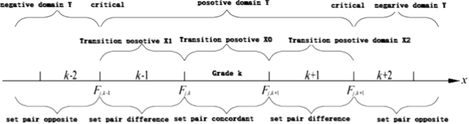
The relationship between set pair of concordant, difference, opposite, and extension set theory domain
Comprehensive indicator’s weight and correspondent membership degree μk (p) are calculated respectively by using the following equations.
$$\mu_{k} = \sum\limits_{j = 1}^{M} {w_{j} \mu_{k} (x_{ij} )}$$(11)in which, wi is indicator weight. The corresponding assessment criteria are defined as,
$$K = \max \left\{ {\mu_{1} ,\mu_{2} , \cdot \cdot \cdot ,\mu_{m} } \right\}$$(12)in which, K refers to determined evaluation grade.


Case Study
River background and data sources
The Huangchuan river is a tributary on the south bank of the Huaihe River, which is originated from the northern foot of Dabie Mountain and flows through Xinxian, Guangshan and Huangchuan county, empties into the Huaihe River at the west of Sihetai village. The total length of the main channel is 140 km, and the basin area covers 2400 km2. The upper reach of the Huangchuan river flows through the steep Dabie Mountains, the middle reach pass through hilly area with gentle slope. The region below Huangchuan is plain area and belongs to agricultural and industrial region. In the Huangchuan river basin, the mountain area amounts to 75%. The overall terrain is high in south and low in north. The trend of terrain is inclined from southwest to northeast. The land surface elevation varies from 35 to 1010 m. The average annual runoff of the river is 1200 million m3. The annual average suspended sediment transport is 216,000 t. Annual sediment transport modulus is 132 t/(km2). A schematic diagram of the river system in the Huangchuan basin is shown in Fig. 4.

Schematic diagram of Huangchuan River water system
By the end of 2016, several water projects have been built in the region, there were 1 large reservoir,4 medium-sized reservoirs,10 small reservoirs and many sluice dams in the river basin.
In this paper,14 control sections were used to evaluate the health grades of Huangchuan River. From August to October in 2017, the riparian zone, water quality and biological conditions at 14 control section points were investigated and monitored by the Project Team. Systematical data including water quality, ecosystem status, water resources and flow environment were obtained. We also conducted a questionnaire survey for the public satisfaction on river systematic management. On the basis of investigation and monitoring, the information provided by Xinxian, Guangshan, Huangchuan and Xinyang Water Conservancy Bureau was collected, which could be meet the requirement for basic data. Based on reviewing results using standard methods, the data reliability meets evaluation requirements.
Determination of physical elements model in the entire and section domain
The physical element matrix (R1、R2、R3、R4) and section matrix of river health evaluation both in entire and section domain could be constructed respectively, as follows;
in which, R1、R2、R3、R4 and Rm are the matrix in entire and section domain respectively, N is the grade of evaluation objectives; C is an evaluation characteristic factor.
Ecological health evaluation on Huangchuan River.
In the physical element extension matrix of health evaluation of Huangchuan river, there are 16 evaluation factors. The evaluation concordant physical element is R2017. The methods of set pair and extension coupling are based on Eq. (3)-(10). The evaluation results for different indicators are seen in Table 2.
Comparing with Table 1, it can be seen from Table 2 that water quality category c7, Sewage treatment rate c8 are illness, which means the Huangchuan river water pollution is serious, at same time, it shows low sewage treatment ability. The riparian integrity index c3 is low, which shows that there is no natural buffer zone, lack of ecological barriers between rivers and land, the ecological function is weak. Low self-regulation ability leads to weak sewage interception and low sewage load capacity as well as low self purification. The evaluation result of satisfaction index of ecological flow c4 shows that the water resources in the Huangchuan river basin could meet the ecological water demand in the relevant river reaches without water transfer from outside basin, but, due to serious water pollution, water quality could not meet the requirement, thus, the river health is affected seriously. River channel corridor connectivity index c11 shows that the river channel corridor system connectivity in Huangchuan basin is low. The main reason is that during recent years many reservoirs, sluice gates and water projects have been built. Ecological improvement projects are carried out in the downstream urban areas and many rubber dams have been constructed. Although such projects have played an active role in ensuring river channel ecological water use, urban water use, landscape construction and environmental improvement, it inevitably cuts off the longitudinal connectivity of the river channel, resulting in low connectivity of channel ecological corridors, which in turn leads to the reduction of the effective transfer of flow materials. The river energy and information transition would be affected. The diversity of species would be reduced. Eventually, the level of river health grade of the biodiversity index c10 was reduced.
Indicators c2、c14 fall in sub-health domain. The reason may be related to the unreasonable development of water use and sandstone exploitation, which increases the soil erosion in the riparian zone, results in river channel silt deposition and river channel block up. The flood control standards would be lowered, and the ecological security of the river is threatened.
Inputting the correlation degree in Table 2 and the index weights into formula (11), the integrated correlation degree of the health state of the Huangchuan river can be obtained, see Table 3. The results show that the health degree of the Huangchuan river is sub-health, the main reasons are water resources over-development, low river channel corridor longitudinal connectivity, lack of riparian natural buffer zone and water pollution. The evaluation results are consistent with the present actual situation of the river management. It also shows that the method of set pair and extension coupling model is suitable to carry out river ecological health assessment.
Discussion and conclusions
The paper firstly put forward the standard index system of river health evaluation, which is qualitatively reflection of river health degree, and real description of the river status. The standard index system of river health comprehensively makes consideration of the relevant characteristics such as river morphology, hydrology, environment, habitat elements and human activities.
Then, set pair analysis-extension coupling method was studied. The relationship between set pair and extension could be classified as concordant, different, opposite in different domains. The coupling model of set pair and extension was constructed. Comprehensive indicator’s weight and correspondent membership degree are calculated respectively by using the relevant models.
Taking Huangchuan river as an example, the physical elements model in the entire and section domain were determined. Ecological health evaluation on Huangchuan river was carried out. Through calculation, the evaluation results for different indicators were achieved.
The method of river health assessment based on the coupling evaluation theory of set-pair analysis and extension makes full use of the extension transformation and calculation, which shows the superiority in calculating correlation degree, and can reflect the determination and uncertainty of practical problems. The model comprehensively considers different factors. The present study provides a new idea in solving the problem of determining the different degree of set pair analysis, and obtains more accurate conclusions.
It is shown by the evaluation results that the health status ot the Huangchuan river is unhealthy. It is necessary to take relevant technical measures such as river regulation, pollution control and ecological restoration as soon as possible to improve the river ecological health so that it can be gradually restored to a healthy environment.
In view of illegal encroachment on river channels, low quality of water environment, insufficient environmental flow and serious damage to water ecology, further relevant measures are needed, such as strengthening management of livestock and poultry breeding, improving control of agricultural non-point source and municipal solid waste treatment in Guangshan and Huangchuan counties along the middle and lower reaches of the river, and rising treatment rate of sewage discharge. Therefore, it is necessary to carry out natural resources control and utilization with the aim of improving Huangchuan river ecological health. Through the rational development of water resources, rising water efficiency, realizing water pollution and other measures, the health level of the Huangchuan river would be raised with a view to sustainable water resources development.
Availability of data and materials
All the data and materials in the current study are available from the corresponding author on reasonable request.
References
Bozor O, Ghaddad AS, Mario MA (2014). Multi-objective quantity-quality reservoir operation in sudden pollution.Water resources Management. 28(1): 567–586
Chen LG, Shi Y, Qian X (2014) Hydrology, hydrodynamics and water quality model for impounded rivers. Adv Water Sci 25(6):856–863
Ellmore JR, Baxter CV, Connolly PJ (2015) Spatial complexity reduces interaction strengths in the meta-food web of a river floodplain mosaic. Ecology 96(1):274–283
Erst ST, Olden JD, Schick RS (2012) Characterizing connectivity relationships in freshwaters using patch-based graphs. Landscape Ecol 27(2):303–317
Gao F, Li L, Huang Q (2017) Progress of river health assessment in changing environment. J Adv Water Sci 37(6):81–87
GaoY, Wang H, Wang F(2007) Construction of river health life assessment index system.J Adv water sci 18(2) :252-257
Gibson MJ, Savic DA, Djordjevic S (2016) Accuracy and computational efficiency of 2D Urban Surface flood modelling based on cellular Automata. Procedia Engineering 154:801–810
Ladson AR, White LJ, Doolan JA (1999) Development and testing of an index of stream condition for waterway management in Australia: index of stream condition. Freshw Biol 41(2):453–468. https://doi.org/10.1046/j.1365-2427.1999.00442.x
Lee HW, Bhang KJ, Park SS (2010) Effective visualization for the spatio-temporal trend analysis of the water quality in the Nakdong river of Korea. Eco Inform 5(4):281–292
Li Y, Zhang Y, Ni W (2015) River health assessment based on entropy weighted extension element model. Transact xi’an University Technol 31(2):189–194
Liu Y (2015) Study on coupling repair of river system structure and function[D]. Dalian University of Technology, Dalian, p 2015
Meyer JL (1997) Stream health:incorporating the human dimension to advance stream ecology.J North American Benthol Soc 16:439–447.
Razmkhah H, Abrishamchi A, Torkian A (2010) Evaluation of spatial and temporal variation in water quality by pattern recognition techniques: a case study on Jajrood River ( Tehran, Iran). J Environ Manage 91(4):852–860
Thorpjh TMC, Delong MD (2006) The riverine ecosystem synthesis: bio-complexity in river networks across space and time. River Res Appl 22(2):123–147
Wang M, Jin J, Zhou Y. 2014. Coupling method and application of set pair analysis. BEIJING:Science Press.152–160.
Wei Q, Li Q, Duan L, 2019. River health comprehensive evaluation in the reach of Tieling in Liaohe River protection area. 50 (1) :134-141.
Whited DC, Kimball JS, Lucotch JA (2012) A riverscape analysis tool developed to assist wild salmon conservation across the North Pacific Rim. Fisheries 37(7):305–314
Wohle E (2017) Connectivity in rivers. Prog Phys Geogr 41(3):345–362
Xia JH, Yan ZM (2004) Advances in research of ecological riparian zones and its trend of development. Journal of Hohai University (natural Sciences) 32(3):252–255
Yang Z, Yang K, Li J (2016) Grey cluster river health assessment coupling model based on SPA theory. Journal of Water Resources and Power 42(7):775–782
Zhai J, Xu G, Guo S (2016) Study on the evaluation method of river health based on coordinated development degree. J Hydraulic Eng 34(8):1–5
Zhang J, Dong Z, Sun D (2010) River health evaluation indicator system based on dominant water function partition. J Hydraulic Eng 41(8):883–892
Zhang Xi, Liu Li, Yan Feng (2014) Application of the set pair analysis model based on normal membership in river health evaluation. water resource power. 32 (3):44–46
Zhao KQ (2000). Set pair analysis and its preliminary application.Hangzhou:Zhejiang Sci Technol Press
Acknowledgements
The study was supported by the National Natural Science Fund of China ( No.50579020)
Funding
The study was supported by the Natural Science Fund of China (No.50579020).
Author information
Authors and Affiliations
Corresponding author
Ethics declarations
Conflicts of interest
The author declare that there should be no known competing financial interests or personal relationships that could have appeared to influence the work reported in this paper.
Consent for publication
All the data in the paper can be published without any competing financial interests or personal relationships that could have appeared to influence the work reported in this paper.
Consent to Participate (Ethics)
The author consents to participate in the works under the Ethical Approval and Compliance with Ethical Standards.
Ethics approval
The author declare that there are no known competing financial interests or personal relationships that could have appeared to influence the work reported in this paper.
Additional information
Publisher's Note
Springer Nature remains neutral with regard to jurisdictional claims in published maps and institutional affiliations.
Rights and permissions
Open Access This article is licensed under a Creative Commons Attribution 4.0 International License, which permits use, sharing, adaptation, distribution and reproduction in any medium or format, as long as you give appropriate credit to the original author(s) and the source, provide a link to the Creative Commons licence, and indicate if changes were made. The images or other third party material in this article are included in the article's Creative Commons licence, unless indicated otherwise in a credit line to the material. If material is not included in the article's Creative Commons licence and your intended use is not permitted by statutory regulation or exceeds the permitted use, you will need to obtain permission directly from the copyright holder. To view a copy of this licence, visit http://creativecommons.org/licenses/by/4.0/.
About this article

Cite this article
Zhou, K. Application of set-pair analysis and extension coupling model in health evaluation of the huangchuan river, China. Appl Water Sci 12, 198 (2022). https://doi.org/10.1007/s13201-022-01719-y
Received:
Accepted:
Published:
DOI: https://doi.org/10.1007/s13201-022-01719-y