
Abstract
Hydrometers are widely used in industry for liquid density measurement. It is important to achieve rapid and high accuracy calibration for hydrometers. Based on the Archimedes principle, a fully automatic hydrometer calibration system in NIM was designed using Cuckow’s method. The liquid density of n-tridecane (C13H28)is calibrated with 441 g high-purity fused silica ring as the solid density standard. The buoyancy of hydrometer is measured by static weighing system with resolution 0.01 mg. The alignment between liquid surface and hydrometer scale was achieved by the lifting platform with the positioning accuracy of 10 μm. According to the weighing value of hydrometer in air and liquid, the density correction value at different scales is calculated. Hydrometer covering a full range (650–1500) kg/m3can be calibrated without changing the liquid. Taking the calibration data of PTB as reference, the experimental data show that the measurement uncertainty of this system is better than 0.3 division (k = 2).
1 Introduction
Hydrometers include petroleum hydrometers, alcoholmeters, saccharometers, lactometers, soil hydrometers, and other mass-fixed hydrometers, which use Archimedes’ principle to measure the density or relative density of liquids. That is, when a hydrometer is suspended in a liquid, the weight of the liquid displaced by the submerged portion of the suspended hydrometer is equal to the weight of the hydrometer itself. Therefore, based on the depth that the hydrometer sinks in the liquid, the density and relative density of the liquid, as well as its concentration, may be measured directly with a scale [1,2,3]. The hydrometer has a wide measurement range and a simple structure, which is easy to operate and relatively inexpensive. Thus, applications of the hydrometer are extremely varied, in fields ranging from the petrochemical industry to food and medical sanitation. In order to ensure measurement accuracy, it is necessary to regularly calibrate hydrometers.
Hydrometers are usually calibrated by using a direct comparison approach. This method employs a comparison measurement based on a density standard reference and involves submerging the standard hydrometer and the to-be-calibrated hydrometer in the same calibration liquid, and comparing their submersion levels. The advantages of this method include the use of a simple device and low cost. However, the following deficiencies exist: (1) low measurement efficiency. During the measurement process, it is required that the to-be-calibrated hydrometer is freely suspended in the liquid. Since each hydrometer measures only a relatively narrow range of densities, for a full range of measurement, i.e., (650–2000) kg/m3, calibration of each density point requires a liquid with a specified density, resulting in the need to prepare over 200 different liquids; (2) these liquids are corrosive and toxic. The standard liquids used in the direct comparison approach are toxic, oftentimes consisting of a mixture of petroleum products, an alcohol-water blend, ethyl hydrogen sulfate, sulfuric acid, mercury iodide, or potassium iodide, all of which are harmful to the human body and pollute the environment; (3) measurement uncertainty is not good enough. In the direct comparison approach, because the measurement on hydrometer is taken at the bottom of the meniscus, a deviation in the line of sight during a manual reading may easily result in error, such that the uncertainty of the measurement is scarcely better than 0.4 division of the scale (k = 2).
One important reason we use the direct comparison approach for hydrometer calibration is that the previous density traceability system in National Institute of Metrology, China (NIM) is based on liquid density reference, such as pure water. With the development of science and technology, the density traceability system gradually transitioned from liquid density reference to solid density reference. In particular, due to advances in the precise measurement of Avogadro’s constant to support the new quantum-based definition of the kg, the XRCD method was developed. This technique utilized solid density reference using a single-crystal silicon sphere of high purity and reduced measurement uncertainty to 2 × 10⁻⁸. The establishment of the solid density reference provided new methods and approaches for the precise measurement of liquid density and calibration of hydrometer [4,5,6]. Using the Cuckow’s calibration method, this paper investigates a fully automatic calibration system for the hydrometer, which allows rapid and accurate calibration of (650–1500) kg/m3 full-range hydrometer without using different liquids [7,8,9,10].
2 The Mathematical Model of Hydrometer Calibration
Cuckow’s method based on Archimedes’ principle is used for hydrometer calibration. The steps are as follows.
2.1 Liquid Density Measurement
Hydrometer calibration is performed using the principle of hydrostatic weighing. The first step is determining the density of the liquid in which the hydrometer is placed. A highly stable solid with a known density (e.g., a silicon ring, silicon cylinder, fused silica ring, or fused silica cylinder) is employed as the density standard. Using the buoyancy calculation formula, the reading of the balance (wSi_L) when weighing the solid density standard in the liquid may be expressed as
where mSi is the mass of the solid density standard, kg; vSi is the volume of solid density standard at 20 °C, m3; βSi is the expansion coefficient of solid density standard, in °C−1; ρL(t) is the density of the standard liquid at temperature t, kg/m3; ρwe is the density of the weight, kg/m3; and ρair is the density of air [11], kg/m3. Thus, the standard liquid density at temperature t can be expressed as
2.2 Weighing Hydrometer in Air
The hydrometer is weighed in air, under the effects of aerostatic buoyancy and gravity. Its weight wair, as shown by the reading on balance is
where mHy is the mass of hydrometer in vacuum, kg;v1 and v2, m3, are the two volumes of the hydrometer, as shown in Fig. 1; αv is the expansion coefficient of hydrometer, °C−1; ta is air temperature, °C; ρair is air density, kg/m3; ρwe is the density of weight, kg/m3.
2.3 Weighing Hydrometer in Liquid
The to-be-calibrated scale is used as a boundary to divide the hydrometer into an upper portion and a lower portion, as shown in Fig. 1, with the upper and lower portions at 20 °C having volumes of v1 and v2, respectively.
The hydrometer is immersed in a standard liquid. A balance is used to measure the weight of hydrometer in this standard liquid at temperature t. Assuming that the contact angle of the liquid is zero degrees, the weight wLiq is
where d is the stem diameter of hydrometer, m; γliq(t) is the surface tension of the standard liquid, N/m. Assuming the hydrometer is placed in a liquid at 20 °C, and the to-be-calibrated scale aligns well with the liquid surface, then the density of the liquid ρ(tR) satisfies the equation
where γ(tR) is the surface tension of the liquid, N/m. Based on Eqs. (1)–(5), and assuming that second-order or higher-order variables can be reasonably neglected, the density of the liquid ρ(tR) is calculated as:
The correction value of the current measuring scale is calculated as
where ρnominal is the nominal value of the measuring scale of the hydrometer, kg/m3.
3 Hydrometer Calibration System Design
The hydrometer calibration system include a weighing unit, a temperature measurement and control unit, and a liquid surface alignment control unit, as in Fig. 2.

Design schematic of hydrometer calibration in NIM
The design of these three parts are described in detail below.
3.1 Weighing Unit
The weighing unit includes a high-accuracy electronic comparator, a load switching mechanism, and a suspension system, as shown in Fig. 3. The electronic comparator is a Mettler Toledo XP505 (measurement range: 520 g, resolution: 0.01 mg), which is used in conjunction with class E1 weights. The hydrometer is loaded by hanging it under the comparator XP505. The measurement range of the hydrometer is (650–1500) kg/m3; its maximal total length is 400 mm, where the maximal length of stem is 200 mm; the maximal diameter and bulb section of stem is 5 mm and 41 mm, respectively; and maximal weight of hydrometer in air is 243 g.

Weighting module with automatic load switching function
The solid density standard consists of a fused silica ring of high purity, which has an outer diameter of 86 mm, an inner diameter of 56 mm, and a height of 60 mm. Its volume, calibrated by the Physikalisch-Technische Bundesanstalt (PTB) in Germany, is (200.37282 ± 0.00050) cm3, and its mass is (441.29218 ± 0.00020) g. The solid density standard is loaded to the comparator XP505 via two metallic wires, each with a diameter of 0.3 mm, and a suspension system made of stainless steel. During measurements, the hydrometer traverses the ring-shaped solid density standard, thus ensuring that the density and temperature of the liquids at the location of the ring are consistent with them near hydrometer.
Hydrometer and solid density standard are weighed using the same comparator, and to make alternate loading possible, forward and backward ball screws (formed by the combination of two ball screws) are used, respectively, which are driven by a servo motor and a small planetary reducer. Because the directions of movement of the ball screws are opposed to one another, alternate loading of the hydrometer and the solid density standard to the comparator XP505 can be performed.
n-tridecane (C13H28) is usually used as standard density liquid. The density of n-tridecane is approximately 756 kg/m3 at 20 °C. If the nominal value of hydrometer is less than 756 kg/m3, hydrometer will float in the liquid and cannot sink. In order to calibrate hydrometer below n-tridecane density, a stainless-steel ring is used on stem as ballast, which is hung to the balance with suspension device and platinum wire together when first zero weighing is performed.
Because the weighing measurement is carried out in air by using an ABA substitution method, the air buoyancy of the weight needs to be considered. The Vaisala PTU300 is used to measure air temperature, humidity, and pressure, with permissible deviations of ± 0.2 °C, ± 0.30 hPa, and ± 1.7%RH, respectively. Current air density is calculated based on the CIPM-2007 equation for air density [11], and air buoyancy is determined. Further, for stable measurement of the electronic comparator with high precision, a windshield is installed covering the entire weighing unit, a vibration-isolation foundation is used, and temperature control for the entire room is provided by an air conditioner, within(20 ± 2) °C.
3.2 Temperature Control and Measurement Unit
Temperature stability is a key factor affecting the calibration uncertainty of hydrometers. Given the Tamson TV7000 as the basis for designing thermostatic module, the volume of the water bath is 70 L, and a glass container with a diameter of 200 mm is installed inside to store the liquid with standard density (i.e., C13H28, or n-tridecane). A dual-cycling system is employed to perform temperature control, in which the Tamson TLC15 acts to adjust the cooling process. To facilitate the stability control of the liquid surface when the hydrometer is calibrated, a rotating speed control stirrer is added to the TV7000, which is configured to adjust stirring speed. Further, a valve is installed at the bottom for internal liquid discharge. The glass container storing C13H28 is installed with a platinum resistance thermometer (Ametek DTI1000), having a permissible measurement deviation of ± 0.01 °C.
The tray and the connection rods used in the installation of the solid density standard are all made of stainless steel, which has high thermal conductivity, and the connection rods will be partially in liquid and partially in air during raising and lowering of the liquid surface. In order to ensure temperature stability of the liquid environment, the portion of the connection rods that touches the liquid surface is made of Teflon.
3.3 Scale Alignment Unit
When calibrating the hydrometer, the liquid surface needs to be lifted up or down to align with each to-be-calibrated scale. An electric lift is applied to move the TV7000 water bath vertically, as shown in Fig. 4. The lift works as follows: the Mitsubishi servo motor drives the planetary reducer, the synchronous belt is propelled and three sets of ball screws are controlled to synchronously drive the water bath up and down. The three sets of ball screws traverse a distance of 500 mm, and the location precision is 10 μm, which keeps the platform stable and ensures that the formation of the meniscus has high repeatability. The lifting platform can be controlled by computer or manually method: (1) the computer-controlled component involves sending a preset number of pulses to the servo motor; (2) the manually controlled component consists of a manual pulse generator connected to the servo motor. A pulse command may be transmitted manually, and in combination with the CCD image system, alignment between the liquid surface and the scale of the hydrometer can be accurately controlled. Via observation with the CCD camera, the liquid surface may be aligned with the to-be-calibrated scale of the hydrometer such that when the surface approaches the scale of the hydrometer, the water bath lifting system is shut down. Fine adjustments are then performed manually in order to precisely align the liquid surface with the scale.

Lifting platform driven by stepper motor
3.4 CCD Image Acquisition Unit
The optical system delivers images of scale to CCD image sensor, and as the front end of the image collection, the performance parameters of the optical system directly determine image collection quality. The field of view is 13 mm × 10 mm, the distance from the stem of hydrometer to CCD image sensor is approximately 600 mm, and the Gaussian equation based on the coaxial optical system is
where u is the object distance, v is the image distance, and u + v = 600 mm. A 1/2″ megapixel CCD sensors applied, with a photosensitive surface height of 4.8 mm, and a magnification factor of β = 4.8 mm/10 mm = 0.48. The focal distance f of the objective lens is
Based on the diffraction limit and the definition of Rayleigh’s rule, the resolution of the objective lens σL can be calculated as
where the relative aperture is F = f/D, D is the entrance pupil diameter of the objective lens, and λ is the wavelength of the incident light. This equation indicates that the resolution of the objective lens is in direct proportion to the size of the relative aperture. Therefore, an objective lens with a relatively small aperture should be selected. When the F value of the objective lens is 3 and the average wavelength of the optical source λ is 585 nm, the resolution of the objective lens σL is 2.1 μm.
The theoretical resolution σS of the CCD image sensor is:
where LC is the length of the smallest pixel of the CCD image sensor, and β is the magnification factor of the optical system. Because the minimum pixel dimension of the CCD image sensor adopted in this system is 5.5 μm × 5.5 μm and β is 0.48, the theoretical resolution σS of the CCD image sensor is 23.0 μm. The theoretical resolution σ0 of entire optical system is calculated as
Therefore, this CCD image system can effectively improve the alignment accuracy of the liquid surface with the scale of hydrometer.
The entire calibration system uses a programmable logic controller (PLC), thus allowing the computer to collect weight data, temperature data, and CCD images. In addition, vertical movement of the electric lifting platform is controllable.
4 Experiment and Uncertainty Budget
4.1 The Temperature Stability of Thermostat
The thermostatic performance of the liquid environment is the most important technical indicator of the Cuckow’s system. Given this, the thermostatic properties of the water bath, primarily including short- and long-term temperature stability, must be measured. The temperature stability curve after the stabilization of the liquid temperature is shown in Fig. 5.

Temperature curve of water bath
Data analysis of liquid temperature shows that the combined TV7000/TLC15 thermostatic control system stabilizes the liquid temperature within ± 10.0 mK during a prolonged experimental run, which satisfies the thermostatic requirements of the Cuckow’s measurement method. Experiments, however, indicate the existence of relatively large temperature pulses, both at the moment that the temperature control system is initiated and when the stirrer is switched on. The reason of the temperature pulses at the moment that the temperature control system is initiated is due to the fact that default parameters of TV7000 are used, including a heating power of 100 W and a duration of 1 min, which are very large thermal shocks for a stabilized liquid environment of 10 mK. The temperature fluctuation occurring when the stirrer is turned on is caused by the rapid mechanical abrasion of the stirrer, which generates heat that warms the liquid. Therefore, during measurements, these two heating zones should be avoided, and measurements need to be taken after the temperature has stabilized.
4.2 Density-Temperature Characteristics of n-Tridecane (C13H28)
Prior to the hydrometer calibration, the silicon ring must be loaded in order to measure the density and temperature of n-tridecane. There is a time difference between these two measurements, during which the temperature, and hence the density, of the n-tridecane may vary. To analyze the magnitude of this variation, the density of n-tridecane within a temperature range of (19–21) °C is measured, shown in Fig. 6.

n-tridecane liquid density versus temperature curve
The experimental data indicate that there is basically a linear relationship between the density and temperature of n-tridecane (C13H28):
Given that the liquid temperature difference between the liquid density measurement and the hydrometer calibration is often within ± 2 mK, the relative error of the liquid density measurement at 20 °C can be calculated using the equation below
Therefore, based on the difference between the two temperatures, the liquid density must be corrected. The average relative difference between density values calculated using the fitting equation and measurement values was found to be 4.23 ppm, indicating that, given the temperature of a liquid, the liquid density of C13H28 can be calculated using a fitting method based on the equation. Thus, it is not necessary to perform liquid measurement each time; however, due to the drift of liquid density, this curve needs to be recalibrated each month.
4.3 Hydrometer Calibration and Comparison
To validate the effectiveness of the hydrometer calibration system in NIM based on the Cuckow’s method, 4 hydrometers were calibrated, and calibration data provided by the Physikalisch-Technische Bundesanstalt (PTB, Germany) were used as Ref. [12,13,14,15]. The hydrometer data are shown in Table 1.
The comparison results are shown in Figs. 7, 8, 9 and 10, and En ratio is used in this proficiency testing between two labs [17].

Comparison data (ID: 1862)

Comparison data (ID: 15)

Comparison data (ID: 122)

Comparison data (ID: 1704)
The comparison data indicate that the measurement values are equivalent to the PTB measurement data. Thus, the effectiveness of the hydrometer measurement system based on the Cuckow’s method is validated.
4.4 Uncertainty Budget
Based on measurement principles, the calibration of the hydrometer consists of two steps: measuring the liquid density and weighing the hydrometer. Therefore, to determine the uncertainty of the hydrometer calibration, the uncertainty of the liquid density measurement first needs to be analyzed [16].
-
(1)
Uncertainty budget on n-tridecane (C13H28) density measurement
The mathematical model for measuring the liquid density is
Define
A partial derivative is derived for this equation, and taking into consideration measurement repeatability, A-type standard uncertainty is introduced. This yields the equation for calculating the uncertainty of the liquid density standard:
where
The calculation data are shown in Table 2.
-
(2)
Uncertainty budget on hydrometer calibration
The mathematical model for hydrometer calibration is
Define
Thus, the above calculation equation can be rewritten as
A partial derivative is derived for this equation, and, taking into consideration measurement repeatability, A-type standard uncertainty is introduced. This yields the equation for calculating the uncertainty of hydrometer calibration:
where
The calculation data are shown in Table 3.
The division of hydrometer for test is 0.2 kg/m3, then if expressed in units of division values, the expanded combined uncertainty is 4.18E−02/0.2 = 0.209 division. Therefore, the Cuckow’s method can be applied to perform a full-range calibration of the hydrometer, with an uncertainty better than 0.3 division (k = 2).
5 Conclusion
-
1.
Using a fused silica ring of high purity as the solid density standard and based on Archimedes’ principle, the Cuckow’s method was applied to calibrate the hydrometer. This technique required only one type of liquid to calibrate the full-range hydrometer.
-
2.
A hydrometer calibration system consisting of a weighing unit (resolution: 0.01 mg), temperature-control unit (permissible measurement deviation: ± 0.01 °C), and scale alignment unit was designed, and the two steps of weighing the hydrometer in air and in liquid were completed. In addition, the alignment between the liquid surface and the scale was performed based on the CCD image collection system, with a mechanical location precision of 10 μm.
-
3.
Experimental data indicated that there is linear relationship between the density of n-tridecane (C13H28) and temperature, within the range of (19–21) °C. The relative difference between density values calculated using the fitting equation and actual measurement values was found to be 4.23 ppm. Using Physikalisch-Technische Bundesanstalt (PTB) data as reference, the hydrometer calibration system in NIM was validated. The expanded uncertainty was 0.3 division value (k = 2).
Abbreviations
- w Si_L :
-
Weighing value of solid density standard in C13H28 (kg)
- m Si :
-
Mass of the solid density standard (kg)
- v Si :
-
Volume of solid density standard at 20 °C (m3)
- β Si :
-
Expansion coefficient of solid density standard (°C−1)
- ρ L(t):
-
Density of the standard liquid at temperature t (kg/m3)
- ρ we :
-
Density of the weights for weighing (kg/m3)
- ρ air :
-
Air density during the weighing (kg/m3)
- w air :
-
Weighing value of hydrometer in air (kg)
- m Hy :
-
Mass of hydrometer in vacuum (kg)
- v 1 and v 2 :
-
Two volumes of hydrometer, as shown in Fig. 1 (m3)
Fig. 1 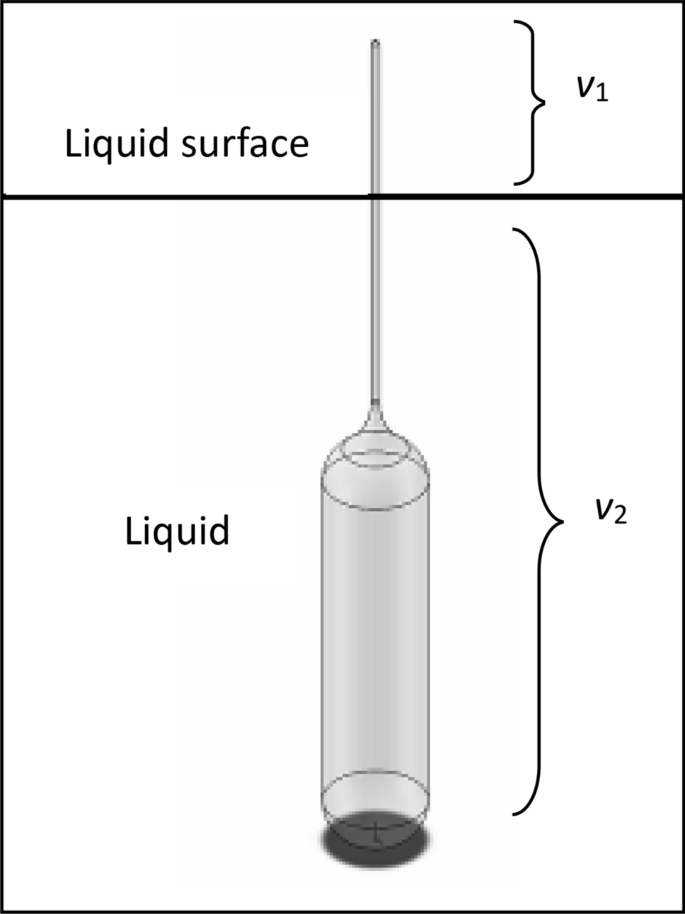
The to-be-calibrated hydrometer
- α v :
-
Expansion coefficient of hydrometer (°C−1)
- t a :
-
Air temperature during measurement (°C)
- w Liq :
-
Weighing value of hydrometer in liquid at temperature t (kg)
- d :
-
Stem diameter of hydrometer (m)
- γ liq(t):
-
Surface tension of standard liquid (N/m)
- ρ(t R):
-
Density of liquid at reference temperature tR (kg/m3)
- γ(t R):
-
Surface tension of liquid (N/m)
- ρ nominal :
-
Nominal value of measuring scale on hydrometer (kg/m3)
- Δρ :
-
Correction value of current measuring scale (kg/m3)
- u :
-
Object distance (mm)
- v :
-
Image distance (mm)
- f :
-
Focal distance f of objective lens (mm)
- σ L :
-
The resolution of objective lens (μm)
- F :
-
The relative aperture (/)
- D :
-
Entrance pupil diameter of objective lens (mm)
- λ :
-
Wavelength of incident light (nm)
- σ S :
-
Theoretical resolution of CCD image sensor (μm)
- L C :
-
Length of the smallest pixel of CCD image sensor (μm)
- β :
-
Magnification factor of optical system (/)
- σ 0 :
-
Theoretical resolution of entire optical system (μm)

References
Stott V 1938 Hydrometers, in The Science of Petroleum, ed A E Dunstan (London, Oxford University Press) vol III p 2322-7.
ISO 649-11981Laboratory glassware-density hydrometers for general purposes-specification.
ISO 649-2 1981 Laboratory glassware-density hydrometers for general purposes-test methods and use.
Nicolaus R A and B onsch G, Absolute volume determination of a silicon sphere with the spherical interferometer of PTB Metrologia 42 (2005) 24-31.
Fujii Kenichi, Present State of the Solid and Liquid Density Standards Metrologia 41 (2004) S1-S15.
Nicolaus R A, Fujii K, Primary Calibration of the Volume of Silicon Spheres Meas Sci Technol 17 (2006) 2527-2539.
Cuckow F W, A new method of high accuracy for the calibration of reference standard hydrometers J. Chem. Ind. 68 (1949) 44-9.
Lee Y J, Chang K H, and Oh C Y, Automatic Alignment Method for Calibration of Hydrometers Metrologia 41 (2004) S100-S104.
Lorefice S and Malengo A, Calibration of Hydrometers Meas. Sci. Technol.17 (2006) 2560-2566.
Aguilera, J., Wright, J., and Bean, V., Hydrometer Calibration by Hydrostatic Weighing with Automated Liquid Surface Positioning Meas. Sci. Technol. 19 (2008) 015104.
Picard A et al. 2008 Revised formula for the density of moist air (CIPM-2007) Metrologia 45 149-155.
PTB Calibration Certificate 2013 PTB-3.23-2013A009-1.
PTB Calibration Certificate 2013 PTB-3.23-2013A009-2.
PTB Calibration Certificate 2013 PTB-3.23-2013A009-3.
PTB Calibration Certificate 2013 PTB-3.23-2013A009-4.
International Organization for Standardization 1996 Guide to the Expression of Uncertainty in Measurement, (Switzerland, International Organization for Standardization).
ISO/IEC 17043:2010 Conformity assessment-General requirements for proficiency testing.
Acknowledgements
Thanks to Dr. Horst Bettin and Mr. Hans Toth of the PTB (Physikalisch-Technische Bundesanstalt, Germany) for their guidance and support. This project was supported by grant from the National Natural Science Foundation of China (No.51475440).
Author information
Authors and Affiliations
Corresponding author
Additional information
Publisher's Note
Springer Nature remains neutral with regard to jurisdictional claims in published maps and institutional affiliations.
Rights and permissions
Open Access This article is licensed under a Creative Commons Attribution 4.0 International License, which permits use, sharing, adaptation, distribution and reproduction in any medium or format, as long as you give appropriate credit to the original author(s) and the source, provide a link to the Creative Commons licence, and indicate if changes were made. The images or other third party material in this article are included in the article's Creative Commons licence, unless indicated otherwise in a credit line to the material. If material is not included in the article's Creative Commons licence and your intended use is not permitted by statutory regulation or exceeds the permitted use, you will need to obtain permission directly from the copyright holder. To view a copy of this licence, visit http://creativecommons.org/licenses/by/4.0/.
About this article

Cite this article
Wang, J., Liu, X., Shi, W. et al. A Fully Automatic Calibration System for Hydrometers in NIM. MAPAN 36, 259–268 (2021). https://doi.org/10.1007/s12647-020-00426-w
Received:
Accepted:
Published:
Issue Date:
DOI: https://doi.org/10.1007/s12647-020-00426-w