Computational aspects of infeasibility analysis in mixed integer programming

Abstract

The analysis of infeasible subproblems plays an important role in solving mixed integer programs (MIPs) and is implemented in most major MIP solvers. There are two fundamentally different concepts to generate valid global constraints from infeasible subproblems: conflict graph analysis and dual proof analysis. While conflict graph analysis detects sets of contradicting variable bounds in an implication graph, dual proof analysis derives valid linear constraints from the proof of the dual LP’s unboundedness. The main contribution of this paper is twofold. Firstly, we present three enhancements of dual proof analysis: presolving via variable cancellation, strengthening by applying mixed integer rounding functions, and a filtering mechanism. Further, we provide a comprehensive computational study evaluating the impact of every presented component regarding dual proof analysis. Secondly, this paper presents the first combined approach that uses both conflict graph and dual proof analysis simultaneously within a single MIP solution process. All experiments are carried out on general MIP instances from the standard public test set Miplib  2017; the presented algorithms have been implemented within the non-commercial MIP solver SCIP and the commercial MIP solver FICO Xpress.

1 Introduction

In the last few decades, mixed integer programming (MIP) has become one of the most important techniques in Operations Research. The general framework of mixed integer programming was successfully applied to many real world applications, e.g., chip design verification [2], scheduling [30, 36, 47], supply chain management [25, 52], and gas transport optimization [22, 31] to mention only a few. A lot of progress has been made in the performance of general MIP solver software; problems that seemed out of scope a decade ago can often be solved in seconds nowadays [5, 13]. The field’s theoretical progress directly stimulated the development of commercial (e.g., CPLEX, FICO Xpress, Gurobi, SAS) and non-commercial (e.g., CBC, SCIP) MIP solvers. In this paper, we will focus on one specific component that is used in almost every state-of-the-art MIP solver: the analysis of infeasible subproblems. Without loss of generality, we consider MIPs of the form

$$\begin{aligned} \min \{ c ^{\mathsf {T}}x \,|\,A x \ge b,\ \ell \le x \le u,\ x _j\in {\mathbb {Z}}\ \forall j\in {\mathcal {I}}\}, \end{aligned}$$

(1)

with objective coefficient vector $c \in {\mathbb {R}} ^{n}$, constraint coefficient matrix $A \in {\mathbb {R}} ^{m\times n}$, constraint left-hand side $b \in {\mathbb {R}} ^{m}$, and variable bounds $\ell , u\in {\overline{{\mathbb {R}}}}^{n}$, where ${\overline{{\mathbb {R}}}}:= {\mathbb {R}} \cup \{\pm \infty \}$. Furthermore, let ${\mathcal {N}}= \{1,\ldots ,n\}$ be the index set of all variables, and let ${\mathcal {I}}\subseteq {\mathcal {N}}$ be the set of variables that are required to be integral in every feasible solution.

By omitting the integrality requirements, we obtain the linear program (LP)

$$\begin{aligned} \min \{ c ^{\mathsf {T}}x \,|\,A x \ge b,\ \ell \le x \le u,\ x \in {\mathbb {R}} ^{n} \}. \end{aligned}$$

(2)

The linear program (2) is called the LP relaxation of (1). The LP relaxation provides a lower bound on the optimal solution value of the MIP (1). This fact is an important ingredient of LP-based branch-and-bound  [18, 35], which is the most commonly used method to solve MIPs. Branch-and-bound is a divide-and-conquer method that splits the search space sequentially into smaller subproblems, which are intended to be easier to solve. During this procedure, the solver may encounter infeasible subproblems. Infeasibility can either be detected by contradicting implications, e.g., derived by domain propagation, or by an infeasible LP relaxation. In this paper’s remainder, we treat an LP relaxation exceeding the current cutoff bound as infeasible. It proves that this subproblem cannot contain a feasible solution of (1) that is better than the currently best-known solution.

Modern MIP solvers try to “learn” from infeasible subproblems, e.g., by conflict graph analysis [1]. More precisely, each subproblem can be identified by its local variable bounds, i.e., by local bound changes that come from branching decisions and domain propagation [46] at the current node and its ancestors. If domain propagation detects infeasibility, one way of conflict learning is traversing the chain of decisions and deductions in a reverse fashion. This procedure allows the reconstruction of the history of bound changes along the root path, thereby identifying explanations for the infeasibility. If it can be shown that a small subset of the bound changes suffices to prove infeasibility, a so-called conflict constraint is generated. This constraint is exploited in the remainder of the search for domain propagation. Consequently, other parts of the search tree can be pruned, and additional bound tightenings can be deducted.

The power of conflict analysis arises because branch-and-bound algorithms often repeat a similar search in slightly different contexts throughout the search tree. Conflict constraints address such situations and aim to avoid redundant work.

Conflict analysis for MIP has its origin in solving satisfiability problems (SAT) and goes back to [39]. Similar ideas are used in constraint programming [e.g., 26, 33, 48]. Integration of these techniques into MIP was independently suggested by [2, 20, 45]. In this paper, we mostly follow the concepts and the notation of [2]. Follow-up publications suggested methods to use conflict information for variable selection in branching [3, 34], to tentatively generate conflicts before branching [6, 8, 11], and to analyze infeasibility detected in primal heuristics [9, 10, 51]. Besides, instead of simply analyzing infeasibility that is derived more or less coincidentally, methods were introduced to generate additional conflict information explicitly [21, 51].

In a preliminary study [49], we examined a vanilla approach of combining conflict graph analysis and dual proof analysis within SCIP. In contrast to conflict graph analysis, dual proof analysis is an LP-based and purely analytic approach that builds on the Farkas lemma [23] to construct a proof of (local) infeasibility. The present paper builds upon this work. Our contribution is twofold: We describe various enhancements for dual proof analysis and present an extensive computational study of the described techniques. On affected instances, the methods presented in this paper improve the performance of SCIP by ${7}{\%}$ in term of solving time and lead to a tree size reduction of ${6.4}{\%}$ compared to the approach reported in [49].

The paper is organized as follows. In Sect. 2, we give a theoretical overview of the analysis of infeasible subproblems. This section covers the concept behind conflict graph analysis and the LP-based theory of dual proof analysis. Section 3 describes three enhancements on dual proof analysis. We will discuss presolving techniques like cancellation and the application of mixed integer rounding functions to strengthen the resulting dual proof constraint. Moreover, we present an update mechanism that allows one to strengthen certain dual proof constraints during the tree search and a filtering method to pick only the most promising dual proof constraints. A comprehensive computational study of the techniques presented in this paper is given in Sect. 4. Additionally, this study contains—to the best of our knowledge—the first computational results within MIP solvers incorporating both conflict graph and dual proof analysis.

2 Infeasibility analysis for MIP

The analysis of infeasible subproblems is widely established in solving MIPs, today. Most state-of-the-art MIP solvers rely either on an adaption of the conflict graph analysis techniques known from SAT or on a pure LP-based approach. Both approaches are strongly connected, as we will argue below.

Assume, we are given an infeasible node of the branch-and-bound tree defined by the subproblem

$$\begin{aligned} \min \{ c ^{\mathsf {T}}x \,|\, A x \ge b,\ \ell ^\prime \le x \le u^\prime ,\ x _j\in {\mathbb {Z}} \, \forall j\in {\mathcal {I}}\} \end{aligned}$$

(3)

with local bounds $\ell \le \ell ^\prime \le u^\prime \le u$. In LP-based branch-and-bound, the infeasibility of a subproblem is typically detected by contradicting implications or by an infeasible LP relaxation. In the following, we describe how both situations can be handled.

2.1 Infeasibility due to domain propagation

Fig. 1

Example of a conflict graph describing all variable bound implications from the branching decisions to the infeasibility $\lambda$ due to propagation. All shown variables are binary

If infeasibility is encountered by domain propagation, modern SAT and MIP solvers construct a directed acyclic graph. The graph represents the logic of how the set of branching decisions led to the detection of infeasibility, see Fig. 1. This graph is called a conflict graph (or implication graph) [39]. The vertices of the conflict graph represent bound changes of variables. The arcs (v, w) correspond to bound changes implied by propagation, i.e., the bound change corresponding to w is based (besides others) on the bound change represented by v.

In addition to the inner vertices that represent the bound changes from domain propagation, the graph features source vertices for bound changes that correspond to branching decisions and an artificial sink vertex representing the infeasibility. Valid conflict constraints can be derived from cuts in the graph that separate the branching decisions from the artificial infeasibility vertex. Based on such a cut, a conflict constraint can be derived; consisting of a set of variables with associated bounds, requiring that at least one of the variables has to take a value outside these bounds in each feasible solution. Note that in general, conflict constraints derived from this procedure have no linear representation if general integer or continuous variables are present. Moreover, by using different cuts in the graph, several different conflict constraints might be derived from a single infeasibility.

A well-established strategy for finding good cuts in the conflict graph is to rely on the so-called First-Unique-Implication-Point (FUIP) [53]. For every level of branching decisions, there exists a FUIP. Zhang et al. [53] have demonstrated that for solving SAT problems using 1-FUIP, i.e., the FUIP of the last branching decision level, is superior to other strategies. In contrast to that, [1] suggested a different strategy for solving MIPs that outperforms using the 1-FUIP solely. The proposed strategy considers the FUIPs of all branching decisions and the corresponding conflict constraints along the path to the root node and chooses the most promising conflict constraints.

2.2 Infeasibility due to an infeasible LP relaxation

During LP-based branch-and-bound, the LP relaxation of each subproblem is solved. If the LP relaxation turns out to be infeasible, the procedure described in Sect. 2.1 cannot be applied directly. The reason is that the LP does not deduce infeasibility from a single constraint but from a potentially large subset of the inequality system (2). Naïvely, one would have to consider all local bound changes as a reason for the infeasibility. This corresponds to adding an edge in the conflict graph from each variable node to the artificial infeasibility node. However, this would not yield a conflict constraint that can be used for pruning elsewhere in the tree. Thus, the naïve reason of infeasibility does not provide additional information for the remainder of the search. Consequently, it is desirable to identify a small set of variables and bound changes sufficient to render the LP infeasible. Such a set of variables and bound changes can be identified by using LP duality theory as reported by Achterberg [1]. In the following, we will refer to such set of variables as initial set. Note, the initial set of variables is not unique in general. In the case of conflict graph analysis, which is a combinatorial approach, sparser conflict constraints are preferred. In the case of binary variables, a conflict constraint encodes that in every feasible solution at least one variable in the constraint has to take a different value compared to the current path along to the root node. Thus, adding a variable would weaken the conflict constraint. A heuristic approach for achieving short conflict constraints is to start from a minimal subset of the initial set of variables that is sufficient to render infeasibility [1]. Note, there might be multiple minimal subsets of the initial set of variables that render infeasibility.

Based on such a minimal subset of variables, the same procedure such as applied to analyze infeasibility due to contradicting variable bounds can be used to derive conflict constraints. Achterberg proposed to pursue the same strategy for analyzing LP-based infeasibility (see the end of Sect. 2.2.2) as for analyzing infeasibility due to domain propagation. That is, considering all FUIPs and choosing the most promising corresponding conflict constraints [1]. In other words, for every FUIP a conflict constraint is generated. Among this set of constraints, a suitable subset for further considerations in the remainder of the solving process is chosen. With this strategy, the overhead introduced by storing and propagating the additional constraints should be reduced.

In this paper, we propose a different strategy considering the LP-based certificate of infeasibility directly, i.e., the so-called initial dual proof constraint. Compared to conflict graph analysis, which is seeded from a single (minimal) subset of the initial set of variables, the initial dual proof constraint encodes all subsets of the initial set of variables that render infeasibility. Thus, it encodes more information. However, this does not mean that a single dual proof constraint dominates all conflict constraints that can be derived from it. As mentioned above, the initial set of variables is not unique in general. Thus, after applying conflict graph analysis, the resulting conflict constraints might contain variables whose bounds have been changed along the root path but are not part of the initial set.

2.2.1 An excursion to duality theory

If solving the LP relaxation detects infeasibility, the proof of infeasibility is given by a ray in the dual space with respect to the zero-objective function.¹ Consider a node of the branch-and-bound tree and the corresponding subproblem of type (3) with local bounds $\ell \le \ell ^\prime \le u^\prime \le u$. The dual LP of the corresponding LP relaxation of (3) is given by

$$\begin{aligned} \max \{ y ^{\mathsf {T}}b + r ^{\mathsf {T}}\{\ell ^\prime ,u^\prime \}\,|\,y ^{\mathsf {T}}A + r = c,\ y \in {\mathbb {R}} ^{n}_{\ge 0},\, r \in {\mathbb {R}} ^{n} \}, \end{aligned}$$

where

$$\begin{aligned} r ^{\mathsf {T}}\{\ell ^\prime ,u^\prime \} := \sum _{\begin{array}{c} j\in {\mathcal {N}}\\ r _j> 0 \end{array}} r _j\ell ^\prime _j+ \sum _{\begin{array}{c} j\in {\mathcal {N}}\\ r _j< 0 \end{array}} r _ju^\prime _j= \sum _{\begin{array}{c} j\in {\mathcal {N}}\\ r ^\ell _j> 0 \end{array}} r ^\ell _j\ell ^\prime _j- \sum _{\begin{array}{c} j\in {\mathcal {N}}\\ -r ^u_j< 0 \end{array}} r ^u_ju^\prime _j \end{aligned}$$

(4)

with $r ^\ell , r ^u\in {\mathbb {R}} ^n_{+}$ representing the dual variable on the finite bound constraints, i.e., $r:= r ^\ell - r ^u$. Note, since every variable $j$ can only be tight in at most one bound constraint, it follows by complementary slackness that either $r ^\ell _j$, $r ^u_j$, or none of them will be different to zero but not both at the same time. For every variable $x _j$ it holds that $r _j= c _j- y ^{\mathsf {T}}A _{\cdot j}$, where $A _{\cdot j}$ denotes the $j$-th column of $A$. By LP theory, each ray $(y,r)\in {\mathbb {R}} ^{m+n}$ in the dual space that satisfies

$$\begin{aligned} \begin{array}{rl} y ^{\mathsf {T}}A + r &{}= 0 \\ y ^{\mathsf {T}}b + r ^{\mathsf {T}}\{\ell ^\prime ,u^\prime \} &{}> 0 \end{array} \end{aligned}$$

(5)

proves infeasibility of (3), which is an immediate consequence of the Lemma of [23]. Hence, if (2) is infeasible, there exists a solution $(y,r)$ of (5).

2.2.2 Analysis of infeasible LPs

It follows immediately from (5) that infeasibility within the local bounds $\ell ^\prime$ and $u^\prime$ is proven by $0 < y ^{\mathsf {T}}b + r ^{\mathsf {T}}\{\ell ^\prime ,u^\prime \} = y ^{\mathsf {T}}b- y ^{\mathsf {T}}A \{\ell ^\prime ,u^\prime \}$. Therefore, the inequality

$$\begin{aligned} y ^{\mathsf {T}}A x \ge y ^{\mathsf {T}}b \end{aligned}$$

(6)

has to be fulfilled by all feasible solutions. Since (6) is a non-negative aggregation of globally valid constraints, it is globally valid too. In the following, this type of constraint will be called dual proof constraint. The dual ray is effectively a list of multipliers on all constraints that are represented in the LP relaxation, such as model constraints (needed by the problem formulation) or additional valid global inequalities, e.g., cutting planes, conflict constraints, and dual proof constraints. Thus, aggregating the constraints according to the multipliers leads to a globally valid but redundant constraint. However, with respect to the local bounds $\ell ^\prime$ and $u^\prime$ it leads to a false statement, thereby proving that the set described by the constraints is empty inside the local bounds. The property of proving infeasibility with respect to at least one set of local bounds distinguishes dual proof constraints from arbitrary constraint aggregations. It is used as some kind of natural “filtering” among the infinitely many different possible constraint aggregations.

In general, infeasibility analysis can also be applied as explained in this paper if locally valid inequalities are present. Here, we assume the corresponding dual multiplier to be 0. The resulting dual proof might not prove local infeasibility anymore. In that case, the analysis of the infeasibility is stopped immediately. Modifications of infeasibility analysis that also incorporate locally valid inequalities are described by [12, 50].

The situation of local infeasibility can be exploited as follows: Either one starts conflict analysis as described in Sect. 2.1 from the set of local bounds, or one considers only the weights given by the dual ray on the model constraints [43, 44]. If those are aggregated with respect to the dual multipliers, omitting the local bounds, we derive a new globally valid constraint, which can be used for domain propagation. We refer to the latter as dual proof analysis and to the outcome of this approach as dual proof constraint. For the remainder of the paper, we will refer to the classical conflict analysis as described in [1] as conflict graph analysis in order to better disambiguate the two concepts. We will speak about the analysis of infeasible subproblems if we refer to both concepts together.

Fig. 2

Illustration of an infeasibility proof. The polytope $P = \{x \in {\mathbb {R}} ^3\;|\; A x \ge b,\ 0 \le x _j\le 1 \text { for } j= 1,2,3\}$ representing the convex hull of the global problem $\min \{0^{\mathsf {T}}x \;|\; A x \ge b,\ x \in \{0,1\}^3\}$. After branching in $x _3$, the subproblem with $x _3 = 0$ can be proven to be infeasible due to an infeasible LP relaxation. The resulting dual proof constraint is $x _3 \ge \frac{2}{3}$ which lead to the global bound deduction $x _3 \ge 1$

An example of an infeasible LP after branching on one variable and the resulting dual proof constraint can be found in Fig. 2. In this case, a single bound change is derived, but in general, the resulting constraint can be directly used for domain propagation during the remainder of the search.

In practice, a dual proof constraint of type (6) is expected to be dense, and therefore, it might be worthwhile to search for a sparser infeasibility proof. Therefore, we will discuss in the following how this constraint can be sparsified and strengthened via dual proof analysis. Both the original and strengthened dual proof constraint can be used as a starting point for conflict graph analysis, which is already described for infeasibility due to domain propagation in Sect. 2.1.

Dual proof analysis Dual proof analysis denotes the modification of a dual proof constraint (6) aiming to sparsify and strengthen the proof of infeasibility. In general, all presolving techniques that apply to a single constraint [e.g., 2, 4, 46], can be used. In Sect. 3, we will especially elaborate on presolving reductions that preserve the local proof of infeasibility. The outcome of dual proof analysis is a single linear constraint that can be used in the remainder of the search to derive further bound deductions and prove the infeasibility of other parts of the tree. Further, it is a starting point for the conflict graph analysis. Dual proof constraints are directly derived from the LP relaxation. In contrast to conflict constraints derived from conflict graph analysis, dual proof constraints do not incorporate any knowledge about integrality or inferences of variables. Therefore, dual proof constraints are only considered for domain propagation. Thus, they do not enter the LP relaxation.

Conflict graph analysis To use the concept of a conflict graph as described in Sect. 2.1, one needs an initial, preferably small, reason for infeasibility. Such encoding of infeasibility can be constructed from an infeasibility proof of type (6): It suffices to consider all local bounds that have a nonzero coefficient in (6). The vertices of the conflict graph that correspond to those local bounds are then connected to the artificial sink representing the infeasibility; global bounds are omitted. Conflict graph analysis can be applied as described in Sect. 2.1.

To strengthen this procedure, one can sparsify the proof of infeasibility  (6) by a heuristic introduced by [1]. The heuristic relaxes some of the local bounds $[\ell ^\prime ,u^\prime ]$ that appear in the dual proof constraint such that the relaxed local bounds $[\ell ^{\prime \prime },u^{\prime \prime }]$ with $\ell< \ell ^{\prime \prime } \le \ell ^\prime \le u^\prime \le u^{\prime \prime } < u$ still fulfill

$$\begin{aligned} y ^{\mathsf {T}}b + r ^{\mathsf {T}}\{\ell ^{\prime \prime },u^{\prime \prime }\} > 0. \end{aligned}$$

Note, the more bounds can be relaxed, the smaller the initial reason gets and the stronger the resulting conflict constraints.

Fig. 3

Illustration of Example 1

Example 1

A main difference between using a dual proof directly instead of applying conflict graph analysis is the consideration of variables that contribute with their global bound. Consider the following MIP

$$\begin{aligned} \begin{aligned} \max x + y + z&\\ s.t. \quad x + y + 2z&\le 2 \\ x + y - 2z&\le 0 \\ x + y + z&\le 1 \\ x,y,z&\in \{0,1\}. \end{aligned} \end{aligned}$$

An optimal solution of the LP relaxation is $(0,\frac{2}{3},\frac{1}{3})$ with objective value 1. After branching on y, the LP relaxation proves infeasibility of the subproblem with $y = 1$. A valid infeasibility proof, i.e., an unbounded ray in its dual, is $(0, -\frac{1}{2}, -1)$. Following Sect. 2.2.2, the resulting dual proof constraint is $1.5 x + 1.5 y \le 1$. Applying conflict graph analysis leads to a single global deduction: $(y \le 0)$, see Fig. 3b. In contrast to that, propagating the dual proof constraint directly leads to two global bound changes: $(x \le 0) \wedge (y \le 0)$, see Fig. 3c. $\square$

3 Three enhancements for dual proof analysis

Dual proof constraints derived as described in Sect. 2.2.2 can be used directly in the remainder of the search. However, similar to conflict graph analysis, the dual proof constraint can be modified and strengthened. In this section, we describe presolving and updating steps for strengthening dual proof constraints. Moreover, we discuss how filtering steps can decide which dual proof constraint should be applied and which should be rejected.

3.1 Presolving and strengthening

Presolving plays an important role in solving mixed integer programs [e.g., 2, 4, 16, 29, 46]. In this section, we will discuss presolving techniques that can be applied to a single linear constraint preserving the property of proving local infeasibility.

Since we consider MIPs of form $A x \ge b$, only constraints of type $a^{\mathsf {T}}x \ge b _0$ are discussed in the remainder of this section. However, in Sect. 3.2 we will stick to the notation used in the literature and consider constraints of form $a^{\mathsf {T}}x \le b _0$. Note, by scaling with $-1$, each representation can be transformed into the other. Many presolving and strengthening techniques use activity arguments [16]. Formally, the maximal activity of a constraint $a^{\mathsf {T}}x \ge b _0$ with respect to the (local) bounds $\ell , u$ is given by

Analogously, the minimal activity is given by

Moreover, we will denote the violation of a constraint with respect to the (local) bounds $\ell$ and $u$ by . Hence, a constraint proves infeasibility with respect to $\ell$ and $u$ if $\nu _{\text {viol}}(a,b _0,\ell ,u) > 0$.

3.1.1 Cancellation

Cancellation is a presolving technique to reduce the number of nonzero coefficients in a constraint [4]. One way of doing so is the summation of constraints. More precisely, adding an equality constraint to an inequality constraint will preserve the feasible region of an LP or a MIP. The crucial part of this presolving technique is to choose a pair of constraints and a scaling factor for the equality constraint such that the support of the modified inequality is reduced. In this section, we present two variants of cancellation that can be applied to dual proof constraints. Both variants have a linear run time in the size of the support of the modified constraint.

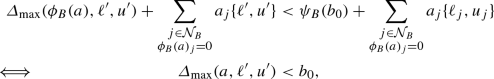
Cancellation with variable bounds Dual proof constraints might contain variables that contribute to the maximal activity with their global bound. Since the local and global contributions to the maximal activity are equal, e.g., $a_j\ell ^\prime = a_j\ell$, those variables can be removed from the infeasibility proof without changing the violation. Let $\ell ^\prime , u^\prime$ be the current local bounds of an infeasible subproblem. Then, a new constraint $\phi _B(a)^{\mathsf {T}}x \ge \psi _B(b _0)$ that still proves local infeasibility can be constructed by

$$\begin{aligned} \phi _B(a)_j&= {\left\{ \begin{array}{ll} a_j, \text { if } j\notin {\mathcal {N}}_{B}\\ 0, \text { otherwise} \end{array}\right. } \end{aligned}$$

(7)

$$\begin{aligned} \psi _B(b _0)&= b _0 - \sum _{j\in {\mathcal {N}}_{B}} a_j\{\ell _j,u_j\}, \end{aligned}$$

(8)

where ${\mathcal {N}}_{B}:= \{ j\in {\mathcal {N}}\;|\; a_j< 0 \text { and } \ell ^\prime = \ell \text { or } a_j> 0 \text { and } u^\prime = u\}$.

Proposition 2

Let $a^{\mathsf {T}}x \ge b _0$ be a globally valid constraint and $\phi _B(a)^{\mathsf {T}}x \ge \psi _B(b _0)$ be constructed as described in (7)–(8) with respect to the local bounds $\ell ^\prime$ and $u^\prime$. Then, the following holds:

• (i) $\nu _{\text {viol}}(a,b _0,\ell ,u) = \nu _{\text {viol}}(\phi _B(a),\psi _B(b _0),\ell ,u)$, and

• (ii) .

Proof

• (i) This follows immediately by construction.

• (ii) We show that for every subproblem defined by $(\ell ^\prime ,u^\prime ) \in {\tilde{{\mathcal {X}}}}$ it follows that $a^{\mathsf {T}}\{\ell ^\prime ,u^\prime \} < b _0$. In other words, every tuple of bound vectors that is proven to be infeasible after applying (7) and (8) is proven to be infeasible by the original infeasibility proof, too. With the following observation

  $$\begin{aligned} \sum _{\begin{array}{c} j\in {\mathcal {N}}_{B}\\ \phi _B(a)_j= 0 \end{array}} a_j\{\ell ^\prime ,u^\prime \} < \sum _{\begin{array}{c} j\in {\mathcal {N}}_{B}\\ \phi _B(a)_j= 0 \end{array}} a_j\{\ell ,u\}, \end{aligned}$$

  where we use the short notation as introduced in (4), it follows immediately that

  

  where $\ell ^\prime ,u^\prime ,\ell ,u$ are chosen to maximize every expression.

$\square$

Proposition 2 shows that using variable bounds to cancel nonzero coefficients in a dual proof constraint leads to a weaker infeasibility proof in general, see Example 3.

Example 3

Let $x + y + z \ge 2$ be a valid dual proof constraint with respect to $\ell ^\prime = (0,0,0)$ and $u^\prime = (0,0,1)$ and $x,y,z \in \{0,1\}$. By construction, the modified constraint will be $x + y \ge 1$. Obviously, $((0, 0, 0),\ (1, 0, 0)) \in {\mathcal {X}}$ but satisfies the modified constraint $x + y \ge 1$, i.e., $((0, 0, 0),\ (1, 0, 0)) \notin {\tilde{{\mathcal {X}}}}$, where ${\mathcal {X}}$ and ${\tilde{{\mathcal {X}}}}$ are defined as in Proposition 2. $\square$

Note that in LP-based branch-and-bound, as it is implemented in most modern MIP solvers, branching is performed only on integer variables. Therefore, we suggest applying the cancellation procedure as described in this section only to continuous variables. In our implementation we pursue a slightly more conservative strategy where only continuous variables are removed that contribute with a global bound to the maximal activity with respect to the current local bounds, i.e., depending on the sign of the coefficient in the dual proof it holds $\ell ^\prime = \ell$ and $u^\prime = u$, respectively. We apply this cancellation as long as ${{\,\mathrm{supp}\,}}(a) > 0.15\cdot \vert {\mathcal {N}}\vert$, where ${{\,\mathrm{supp}\,}}(a) := \{j\in {\mathcal {N}}\;|\;a_j\ne 0\}$ denotes the support of $a^{\mathsf {T}}x \ge b$. This threshold is identical to the default threshold used to decide whether a conflict constraint, i.e., an infeasibility certificate derived from conflict graph analysis, should be accepted.

For the special case of all $j \in {{\,\mathrm{supp}\,}}(a) \cap {\mathcal {I}}$ are binary and all continuous variables contribute with a global bound, i.e., $j \in {{\,\mathrm{supp}\,}}(a) \cap ({\mathcal {N}}\setminus {\mathcal {I}})\ :j \in {\mathcal {N}}_{B}$, we apply a more sophisticated strategy. Consider a maximal set of binary variables ${\mathcal {I}}^{\text {max}} \subset ({{\,\mathrm{supp}\,}}(a) \cap {\mathcal {I}})$ which is not sufficient to prove infeasibility with respect to the local bounds $\ell ^\prime$ and $u^\prime$, i.e.,

but for any binary variable $x _j$ with $j\notin {\mathcal {I}}^{\text {max}}$ it holds

If such a set exists, all continuous variables can be canceled with their global bound without weakening the dual proof if they are never sufficient to prove infeasibility, i.e.,

In that case the assignment of one additional binary variable $x _j$ with $j\notin {\mathcal {I}}^{\text {max}}$ to its current local bound is always needed to prove infeasibility, independently from the assignment of the continuous variables.

Cancellation with variable bound constraints Next to variable bounds that are explicitly given by the problem formulations, modern MIP solvers detect and use so-called variable bound constraints [24].

Definition 4

(Variable Bound Constraint [24]) Let $b^l_{}, b^u_{} \in {\overline{{\mathbb {R}}}}, c \in {\mathbb {R}}$ with $c \ne 0$. A variable bound constraint has the form

$$\begin{aligned} b^l_{} \le x _j+ c x _k \le b^u_{}, \end{aligned}$$

where $x _j$ is a continuous or integer variable and $x _k$ a binary or integer variable.

If $b^l_{} = -\infty$ and $b^u_{}$ finite, the constraint gives an upper bound on $x _j$, while a lower bound on $x _j$ is given if $b^l_{}$ is finite and $b^u_{} = \infty$. A typical example of variable upper bound constraints are so-called big-M constraints $x _j\le Mx _k$, where M is a (usually) huge constant, and $x _k$ is binary. Other typical use-cases are precedence constraints on start time variables in scheduling.

Let ${\mathcal {N}}_{V}\subseteq {{\,\mathrm{supp}\,}}(a)$ be the index of a variable for which a compatible variable bound constraint exists. A variable bound constraint on variable $x _j$ with $a_j> 0$ is compatible if it defines an upper bound. Analogously, a variable lower bound constraint on $x _j$ is compatible if $a_j< 0$. Moreover, let ${\mathcal {V}}$ be an arbitrary set of compatible variable bound constraints with respect to $a_j$ containing, for every $j$, at least one variable bound constraint

$$\begin{aligned} b^l_{j} \le x _j+ c _{jk} x _k \le b^u_{j} \end{aligned}$$

such that $x _k$ is binary or general integer, respectively, and $x _j$ is general integer or continuous, respectively. Since $x _k$ defines a bound on $x _j$, we identify variable bound constraint in ${\mathcal {V}}$ by the tuple (j, k).

Given the sets ${\mathcal {N}}_{V}$ and ${\mathcal {V}}$, one can construct an alternative proof $\phi _{V}(a)^{\mathsf {T}}x \ge \psi _{V}(b _0)$, where

$$\begin{aligned} \phi _{V}(a)_j&= {\left\{ \begin{array}{ll} 0, &{}\text { if } j\in {\mathcal {N}}_{V}\\ a_j- \sum \limits _{\begin{array}{c} k \ne j\\ (k,j) \in {\mathcal {V}} \end{array}} a_kc _{kj},&\text { if } j\notin {\mathcal {N}}_{V}\end{array}\right. } \end{aligned}$$

(9)

$$\begin{aligned} \psi _{V}(b _0)&= b _0 - \sum _{\begin{array}{c} j\in {\mathcal {N}}_{V}\\ (j,k) \in {\mathcal {V}} \end{array}} a_j\{b^l_{j},b^u_{j}\}. \end{aligned}$$

(10)

Proposition 5

Let $a^{\mathsf {T}}x \ge b _0$ be a globally valid dual proof constraint and $\phi _{V}(a)^{\mathsf {T}}x \ge \psi _{V}(b _0)$ be a modified constraint following (9)–(10) with respect to the local bounds $\ell ^\prime$ and $u^\prime$. For every $j\in {\mathcal {N}}_{V}$ with $(j,k) \in {\mathcal {V}}$ and $b^l_{j} = \ell ^\prime _j+ c _{jk} \{\ell ^\prime _k,u^\prime _k\}$ or $u^\prime _j+ c _{jk} \{\ell ^\prime _k,u^\prime _k\} = b^u_{j}$ it holds

$$\begin{aligned} \nu _{\text {viol}}(a,b _0,\ell ^\prime ,u^\prime ) = \nu _{\text {viol}}(\phi _{V}(a),\psi _{V}(b _0),\ell ^\prime ,u^\prime ). \end{aligned}$$

The proof of the proposition follows by construction because only variable bound constraints that are satisfied with equality with respect to the local bounds are used for substitution.

By construction, the substitution of variables with variable bound constraints does not necessarily lead to smaller support in general. However, it can improve the capability of propagating the modified infeasibility proof, as the following examples show.

Example 6

Let $x_1 + x_2 - \frac{1}{2}y \ge 1$, $x_1,x_2 \in \{0,1\}$ with $\ell _j= \ell ^\prime _j= 0, u_j= u^\prime _j= 1$ for $j= 1,2$, $y \in {\mathbb {Z}}$ with $0 \le y \le 4$. Moreover, let $y - 2x_1 \ge 0$ be a variable lower bound constraint of y. Applying (9) and (10) leads to

$$\begin{aligned} \left. \begin{array}{rrrrrrrr} &{} x_1 &{}+&{} x_2 &{}-&{} 0.5y &{}\ge &{} 1 \\ -&{} x_1 &{} &{} &{}+&{} 0.5y &{}\ge &{} 0 \end{array} \right\} \quad \Longrightarrow \quad x_2 \ge 1. \end{aligned}$$

$\square$

Example 7

Let $x_1 + x_2 - z \ge 1$, $x_1,x_2 \in \{0,1\}$ with $\ell _j= \ell ^\prime _j= 0, u_j= u^\prime _j= 1$ for $j= 1,2$, $z \in {\mathbb {R}}$ with $0 \le z \le M$ and $M > 2$. Moreover, let $z - Mw \ge 0$ be a variable lower bound constraint of z with $w \in \{0,1\}$. Applying (9) and (10) leads to

$$\begin{aligned} \left. \begin{matrix} x_1 &{}+&{} x_2 &{}-&{} z &{} &{} &{}\ge &{} 1 \\ &{} &{} &{}+&{} z &{}-&{} Mw &{}\ge &{} 0 \end{matrix} \right\} \quad \Longrightarrow \quad w = 0. \end{aligned}$$

$\square$

In our implementation, we make use of both described cancellation strategies. Firstly, we try to replace continuous and general integer variables with a variable bound constraint that is tight with respect to the local bounds such that no additional nonzero coefficient is introduced. Moreover, we only substitute continuous variables by general integer and binary variables and general integer variables by binary variables. To break ties, we consider the left- and right-hand side of the variable bound constraints (sides closer to zero are preferred) and the variable locks [2] of the substitution variable $x _k$ (more locks are preferred).

Afterward, we cancel continuous variables that contribute to the dual proof’s activity with their global bound following the procedure and case distinction described above.

3.1.2 Updating procedure

During the tree search subproblems are pruned due to infeasibility or because of the corresponding LP is proven to exceed the solution value of the currently best-known solution. This threshold is called the cutoff bound. In general, an LP that is proven to exceed the cutoff bound can be transformed into an infeasible LP by adding a constraint

$$\begin{aligned} c ^{\mathsf {T}}x \le c ^{\mathsf {T}}x ^{\star }, \end{aligned}$$

(11)

where $x ^{\star }$ denotes the currently best-known solution. In the following, we will denote this solution as incumbent solution.

A valid proof that the LP relaxation exceeds the cutoff bound is given by every dual feasible solution $(y,r)$ fulfilling

$$\begin{aligned} y ^{\mathsf {T}}b + r ^{\mathsf {T}}\{\ell ^\prime , u^\prime \}> c ^{\mathsf {T}}x ^{\star } \Longleftrightarrow y ^{\mathsf {T}}b + (c- y ^{\mathsf {T}}A)^{\mathsf {T}}\{\ell ^\prime , u^\prime \} > c ^{\mathsf {T}}x ^{\star }, \end{aligned}$$

(12)

where $r _j$ denotes the reduced costs of $x _j$ for all $j\in {\mathcal {N}}$. A globally valid dual proof constraint can be derived from (12):

$$\begin{aligned} (y ^{\mathsf {T}}A- c)^{\mathsf {T}}x \ge y ^{\mathsf {T}}b- c ^{\mathsf {T}}x ^{\star }. \end{aligned}$$

(13)

This dual proof constraint has to be fulfilled by all improving solutions. Constraint (13) is globally valid since it is a convex combination of all rows $A _{i\cdot }$ and the cutoff constraint (11) scaled by $-1$.

Proposition 8

Let $x ^{\star }$ be the incumbent solution and $(y ^{\mathsf {T}}A- c) x \ge y ^{\mathsf {T}}b- c ^{\mathsf {T}}x ^{\star }$ an infeasibility proof for a bound-exceeding LP with respect to local bounds $\ell ^\prime$ and $u^\prime$. For every feasible solution ${\bar{x}}^{\star }$ with $c ^{\mathsf {T}}{\bar{x}}^{\star } < c ^{\mathsf {T}}x ^{\star }$ the dual proof constraint can be strengthened to $(y ^{\mathsf {T}}A- c) x \ge y ^{\mathsf {T}}b- c ^{\mathsf {T}}{\bar{x}}^{\star }$ by tightening the right-hand side. Afterwards, the strengthened constraint

• (i) still proves infeasibility with respect to $\ell ^\prime$ and $u^\prime$ and

• (ii) is globally valid.

Proof

• (i) $y ^{\mathsf {T}}b + r ^{\mathsf {T}}\{\ell ^\prime , u^\prime \}> c ^{\mathsf {T}}x ^{\star } > c ^{\mathsf {T}}{\bar{x}}^{\star }$

• (ii) By construction $(y ^{\mathsf {T}}A- c) x \ge y ^{\mathsf {T}}b- c ^{\mathsf {T}}{\bar{x}}^{\star }$ is a convex combination of all rows $A _{i\cdot }$ and the strengthened constraint (11) scaled by $-1$. Hence, the dual proof constraint is globally valid. $\square$

In our implementation we use this updating scheme to strengthen dual infeasibility proofs derived from bound-exceeding LPs each time a new incumbent solution is found. Note, since dual proof constraints are only used for domain propagation the strengthening does not directly impact the LP relaxation.

3.2 Mixed-integer rounding

Applying mixed integer rounding (MIR) cuts [41, 42] was proven to be very successful [e.g., 14, 15] when generating strong cutting planes for mixed integer programming. It has been shown [41] that MIR cuts imply Gomory’s mixed integer cuts [28]. The family of mixed integer rounding cuts has a wide range and covers structured and unstructured MIPs. In this section, we will focus on complemented MIR [38] inequalities, and we will discuss how this well-established type of mixed integer rounding function can be used to strengthen dual proofs.

3.2.1 c-MIR inequalities

The MIR procedure strengthens a single linear inequality by rounding the coefficients of integer variables.

Theorem 9

[17] Consider a mixed integer set defined by a single inequality

$$\begin{aligned} {\mathcal {S}} := \{(x,z) \in {\mathbb {Z}} ^n_+ \times {\mathbb {R}} ^p_+ \;|\; a^{\mathsf {T}}x + g^{\mathsf {T}}z \le b\}. \end{aligned}$$

Let $f_0 = b - \lfloor b\rfloor$ and $f_j= a_j- \lfloor a_j\rfloor$. Then the inequality

$$\begin{aligned} \sum _{j= 1}^n \left( \lfloor a_j\rfloor + \frac{\left( f_j- f_0\right) ^+}{1 - f_0}\right) x_j+ \frac{1}{1 - f_0} \sum _{j= 1\,:\,g_j< 0}^p g_jz_j\le \lfloor b\rfloor \end{aligned}$$

(14)

is a valid inequality for conv(S).

For the proof of this theorem, we refer to [17]. Inequality (14) is called MIR inequality. Note, Theorem 9 defines the MIR inequality for nonnegative variables only. However, every variable with at least one finite bound can be shifted into the nonnegative space by complementing with one of its (finite) bounds. Complementing variables can also be used to strengthen the MIR inequality. A variant of the MIR inequality combined with a special scaling parameter was proposed by [38].

Theorem 10

[38] Consider a mixed integer set defined by a single inequality

$$\begin{aligned} {\mathcal {S}} := \{(x,z) \in {\mathbb {Z}} ^n_+ \times {\mathbb {R}} _+ \;|\; a^{\mathsf {T}}x + z \le b,\ x_j\le u_j\, \forall j \in {\mathcal {I}}\}. \end{aligned}$$

Let (T, C) be a partition of ${\mathcal {I}}$ and $\delta > 0$. A complemented-MIR (c-MIR) for S associated with (T, C) and $\delta > 0$ is obtained by complementing variables in C and dividing by $\delta$ before generating the MIR inequality.

$$\begin{aligned} \sum _{j\in T} G\left( \frac{a_j}{\delta }\right) x_j+ \sum _{j\in C} G\left( \frac{-a_j}{\delta }\right) \left( u_j- x_j\right) \le \lfloor \beta _0\rfloor + \frac{z}{\delta (1-f_0)}, \end{aligned}$$

where $\beta _0 = (b - \sum _{j\in C} a_ju_j)/\delta$, $f_0 = \beta _0 - \lfloor \beta _0\rfloor$, and $G(d) = \left( \lfloor d\rfloor + \frac{(f_d - f_0)^+}{1-f_0}\right)$.

In the context of cutting planes, the MIR inequality is usually built from a nonnegative linear combination of valid inequalities. A heuristic how to derive a proper nonnegative linear combination that separates a given point (x, z) was proposed in [38], where (x, z) is valid for the LP relaxation but violates the integrality conditions. Using the dual ray $(y,r)$ yields a nonnegative linear combination that is valid for the global problem, see Sect. 2.2.1. Thus, the MIR procedure can be applied to the resulting proof constraint.

3.2.2 Applying c-MIR to dual proofs

In the following, we will define the partition (T, C) of ${\mathcal {I}}$, such that we always choose the closest bound [38]. Formally, if $\ell \le x \le u$ is the given reference point it follows $C := \{j\in {\mathcal {I}}\;|\; x_j> (u_j- \ell _j)/2\}$ and $T := {\mathcal {I}}\setminus C$.

In contrast to the classical separation procedure, where an LP-valid point should be separated from the convex hull, no such point is given when analyzing a subproblem with an infeasible LP relaxation. Due to this fact, there exists a certain degree of freedom when choosing a reference point that is used for complementing the MIR inequality. The (arbitrary) reference point is used to compute the efficacy of the infeasibility proof before and after applying the c-MIR procedure. We aim to strengthen the initial proof of infeasibility such that it propagates well in the remainder of the search. Since we aim at using globally valid proofs, the global bounds need to be used when complementing the MIR inequality.

The question remains which reference point to use when complementing the MIR inequality. The LP solution of the root node or the incumbent solution is not related to the current subproblem. In contrast to that, ${\hat{x}}$ with

$$\begin{aligned} {\hat{x}}_j= {\left\{ \begin{array}{ll} u_j&{} \text { if } a_j< 0, \\ \ell _j&{} \text { if } a_j\ge 0 \\ \end{array}\right. } \end{aligned}$$

is a natural choice because is related to the variable bounds contributing to the constraint activity. However, always using the bounds contributing to the minimal activity according to the respective signs for complementation might in general lead to weak local proofs, as can be seen from the following lemma. We say an infeasibility proof is stronger (weaker) with respect to a given reference point than another infeasibility proof, if its violation with respect to the given reference point is larger (smaller).

Lemma 11

Let $a^{\mathsf {T}}x \le b$ be a proof of local infeasibility with respect to $\ell ^\prime$ and $u^\prime$ and $\ell ^\prime \le {\tilde{x}} \le u^\prime$ be a reference point minimizing the activity of $a^{\mathsf {T}}x$. Moreover, let $\delta = 1$ and (T, C) and $(T^\prime ,C^\prime )$ be two partitions of ${\mathcal {I}}$ such that $C^\prime \subset C$ and $\vert C \setminus C^\prime \vert = 1$. Further, let $k \in C \setminus C^\prime$ with $a_k < 0$. Assume $(1 - f_k) u_k > u^\prime _k$, $G(a_k) = \lfloor a_k\rfloor$, and $G(-a_k) = \lfloor -a_k\rfloor$, i.e., the fractionality of the coefficient is smaller than the fractionality of the right-hand side in both cases. Then, complementing with $(T^\prime ,C^\prime )$ yields a stronger local infeasibility proof with respect to ${\tilde{x}}$.

Proof

Let $R(x) := \sum _{j\in T} G(a_j) x_j+ \sum _{j\in C^\prime } G(-a_j) (u_j- x_j)$ be the common part of both inequalities after applying the c-MIR procedure

$$\begin{aligned} R(x) + G(a_k) x_k&\le \lfloor \beta _0\rfloor \end{aligned}$$

(15)

$$\begin{aligned} \text {and} \qquad R(x) + G(-a_k) (u_k - x_k)&\le \lfloor \beta _0\rfloor - a_k u_k. \end{aligned}$$

(16)

We show that (15) has a smaller slack than (16) with respect to ${\tilde{x}}$ under the assumption that $(1 - f_k) u_k > u^\prime _k$.

$$\begin{aligned} R({\tilde{x}}) + G(a_k) {\tilde{x}}_k + s_1&= \lfloor \beta _0\rfloor \\ \text {and} \qquad R({\tilde{x}}) + G(-a_k) (u_k - {\tilde{x}}_k) + s_2&= \lfloor \beta _0\rfloor - a_k u_k. \end{aligned}$$

Assume $s_1 < s_2$:

$$\begin{aligned}&G(a_k) {\tilde{x}}_k + s_1 - G(-a_k) (u_k - {\tilde{x}}_k) - s_2&= a_k u_k \\ \Leftrightarrow&G(a_k) u^\prime _k + s_1 - G(-a_k) (u_k - u^\prime _k) - s_2&= a_k u_k \\ \Leftrightarrow&G(a_k) u^\prime _k - G(-a_k) (u_k - u^\prime _k)&> a_k u_k \\ \Leftrightarrow&(\lfloor a_k\rfloor + \lfloor -a_k\rfloor ) u^\prime _k - \lfloor -a_k\rfloor u_k&> a_k u_k \\ \Leftrightarrow&(\lfloor a_k\rfloor - \lceil a_k\rceil ) u^\prime _k + \lceil a_k\rceil u_k&> a_k u_k \\ \Leftrightarrow&-u^\prime _k + \lceil a_k\rceil u_k&> a_k u_k \\ \Leftrightarrow&(1-f_k) u_k&> u^\prime _k \end{aligned}$$

$\square$

Proposition 12

For arbitrary but finite lower bounds $\ell _j\ne 0$ Lemma 11 generalizes to

$$\begin{aligned} u^\prime _k < (1-f_k) u_k + f_k \ell _k. \end{aligned}$$

The proof of the above proposition follows the proof of Lemma 11 whereby inequality (15) changes to $R(x) + G(a_k) (x_k - \ell _k) \le \lfloor \beta _0\rfloor - a_k \ell _k$. Based on the above proposition we propose to use the reference point ${\bar{x}}$ with

$$\begin{aligned} {\bar{x}}_j= {\left\{ \begin{array}{ll} u_j&{} \text { if } a_j> 0 \text { and } \ell ^\prime _j\ge \frac{u_j+ \ell _j}{2}, \\ u_j&{} \text { if } a_j< 0 \text { and } u^\prime _j\ge \frac{u_j+ \ell _j}{2}, \\ \ell _j&{} \text { if } a_j> 0 \text { and } \ell ^\prime _j< \frac{u_j+ \ell _j}{2}, \\ \ell _j&{} \text { if } a_j< 0 \text { and } u^\prime _j< \frac{u_j+ \ell _j}{2}, \\ \end{array}\right. } \end{aligned}$$

instead of using the global upper or lower bound depending on the sign of the respective coefficients, when applying the c-MIR procedure to dual infeasibility proofs. This heuristic relaxes the result of Lemma 11 and Proposition 12 by dropping the dependency on the fractionality of the coefficients.

In our implementation, we either keep the dual infeasibility proof or the derived c-MIR inequality. To estimate which constraint might be most beneficial in the remainder of the search, we consider the efficacy with respect to the described reference point ${\bar{x}}$, see Sect. 4.3 for further details.

3.3 Filtering

Conflict graph analysis and dual proof analysis share the initial reason of infeasibility $y ^{\mathsf {T}}b + r ^{\mathsf {T}}\{\ell ,u\} > 0$ as a common starting point (see Sect. 2). Both techniques follow different paths such that the resulting constraints are of very different nature. Conflict constraints derived from analyzing the conflict graph rely on combinatorial arguments. Consequently, these constraints are not challenging with respect to their numerical properties and expected to be sparse. Here, the shorter the conflict constraint, the stronger it is [32]. This observation becomes more apparent when looking at a conflict constraint from the SAT perspective, i.e., interpreting it as a set of literals that cannot be all satisfied at the same time. Thus, adding a literal weakens the proof.

In contrast, constraints derived from dual proof analysis purely rely on the numerical conditions of the constraint set of the MIP and the properties of the dual proof obtained by solving the infeasible LP relaxation. Therefore, these proofs can be expected to be numerically more challenging and denser than those derived from analyzing the conflict graph. In the case of dual proofs, “sparser is better” does not hold anymore. Therefore, it is essential to pick the most promising infeasibility proofs derived from dual proof analysis. As opposed to conflict constraints derived by conflict graph analysis, dual proof constraints rely on the initial proof’s actual coefficients because these coefficients are needed to define the actual constraint. We filter out dual proof constraints that might lead to numerically unstable propagation steps. This filtering is done by restricting the maximal absolute range of all coefficients. For a given constraint $a^{\mathsf {T}}x \ge b$ we consider the minimal and maximal absolute coefficient which will be denoted by

$$\begin{aligned} {a}_{\min } := \min \{ \vert a_j\vert \;|\;j\in {{\,\mathrm{supp}\,}}(a) \}\quad \text {and}\quad {a}_{\max } := \max \{ \vert a_j\vert \;|\;j\in {{\,\mathrm{supp}\,}}(a) \}. \end{aligned}$$

In our implementation we discard all proof constraints for which the dynamism ${a}_{\max } / {a}_{\min }$ exceeds a threshold of ${1}\mathrm {e}{+8}$.

Dual infeasibility proofs derived by aggregating constraints $A _{i\cdot }$ weighted by a dual ray $(y,r)$ are often dense. From a practical point of view there are two reasons why longer proof constraints are assessed to be inferior against shorter proof constraints, which hold for general constraints as well. It is expected that fewer bound changes on the support of a short constraint are necessary to derive new deductions. Therefore, constraints with small support are expected to propagate “earlier” than constraints with large support. Moreover, there are also technical reasons to prefer constraints with small support. Firstly, dense constraints consume more memory. Secondly, certain types of constraints are much more computationally costly to propagate than others. For example, consider a general linear constraint involving arbitrary variables and coefficients–which is most likely the case for a dual proof. Propagating a general linear constraint $a^{\mathsf {T}}x \ge b$, e.g., by activity based bound tightening [16], is done infeasibility ${\mathcal {O}}(\vert {{\,\mathrm{supp}\,}}\{a\}\vert )$.

To not systematically abolish dense dual proof constraints, we propose a dynamic threshold on the size of its support to decide whether the proof should be accepted and maintained in the remainder of the search or immediately rejected. To this end, we consider the average density of all model constraints $A _{i\cdot }$, which will be denoted by

$$\begin{aligned} {{\,\mathrm{supp}\,}}_{\emptyset }(A) := \frac{\sum _{A _{i\cdot }\in A} \vert {{\,\mathrm{supp}\,}}(A _{i\cdot })\vert }{\vert A \vert }. \end{aligned}$$

Further, let ${\mathcal {C}}$ be the set of all dual proofs currently maintained and $a^{\mathsf {T}}x \ge b$ a new dual proof. We accept the constraint if,

$$\begin{aligned} {{\,\mathrm{supp}\,}}_{\emptyset }({\mathcal {C}} \cup \{a^{\mathsf {T}}x \ge b \}) \le \max \{\alpha {{\,\mathrm{supp}\,}}_{\emptyset }(A),\; \beta \vert {\mathcal {N}}\vert \}, \end{aligned}$$

with $\alpha ,\beta > 0$. By this, we do not restrict the density of a single constraint but rather the average density over the set of maintained dual proofs. Since dense dual proof constraints are expected to cover a larger variety of reasons of infeasibility but are computationally costly during domain propagation, we try to balance both properties. With this strategy, we aim to adjust the threshold dynamically, depending on the actual density of all accepted dual proof constraints. Thus, if sufficiently many sparse dual proof constraints are maintained at the current point in time, we are willing to spend more effort on dense dual proof constraints. This strategy holds as long as the average expected effort does not exceed the dynamic threshold. Note that dual proof constraints with support of size one are immediately transformed into a bound change and, therefore, not included in the average density.

4 Computational study

In this section, we present an extensive computational study on general MIP problems investigating the computational impact of the different ways of analyzing infeasibility in MIP presented in this paper. To evaluate the individual impact of all the different techniques presented in this paper, we will analyze each of them in detail.

In Sect. 4.1, we compare the impact of conflict graph analysis and dual proof analysis. Moreover, we present computational results where both techniques were simultaneously used within the state-of-the-art MIP solvers SCIP and FICO Xpress. To the best of our knowledge, these are the first implementations of a combined approach within a single solver. In Sect. 4.2–4.4 we present individual computational results for all enhancement techniques presented in Sect. 3.

All experiments of Sect. 4.2 were performed with the academic MIP solver SCIP  5.1.0 using SoPlex  3.1.1 as LP solver [27]. The experiments in Sect. 4.1 were conducted with SCIP and FICO Xpress  8.6.3.² To evaluate the generated data the interactive performance evaluation tool³ (IPET) was used. The SCIP experiments were run on a cluster of identical machines equipped with Intel Xeon E5-2690 CPUs with 2.6 GHz and 128 GB of RAM. The FICO Xpress experiments were run on a cluster of identical machines equipped with Intel Xeon E5-2640 CPUs with 2.4 GHz and 64 GB of RAM. A time limit of 7200 seconds was set in either case.

As test set we used the newly released benchmark set of Miplib  2017.⁴

To account for the effect of performance variability [19, 37] all SCIP experiments were performed with three different global random seeds; FICO Xpress experiments were run on three different permutations of the problem. Determinism is preserved because SCIP and FICO Xpress use pseudo-random number generators only. Every pair of MIP problem and seed/permutation is treated as an individual observation, effectively resulting in a test set of 720 instances. We will use the term “instance” when referring to a problem-seed combination or a specific permutation of a problem.

In the following, we present aggregated results for every experiment containing the number of solved instances (S) and the absolute and relative solving times in seconds (T and T_Q) and the number of explored branch-and-bound nodes (N and N_Q). The number of nodes is restricted to instances that were solved to optimality by all considered settings. Absolute numbers are always given for the baseline setting, whereas relative numbers are shown for all other settings. To aggregate the individual observations, a shifted geometric mean [2] is used, where a shift of 1 and 100 is used for solving time and nodes, respectively.

Relative solving times of setting s are defined by the quotient $t_s / t_b$, where $t_s$ is the absolute solving time of setting s and $t_b$ is the absolute solving time of setting b that is used as a baseline. An analogous definition holds for explored branch-and-bound nodes. Thus, numbers less than one imply that setting s is superior and numbers greater than one imply that it is inferior to the baseline setting b. Note, that a relative solving time $t_s / t_b$ corresponds to a speedup factor of $t_b / t_s$.

Besides the results for the benchmark set of Miplib  2017,⁵ that are denoted by all, the tables state the impact on instances that are affected. An instance is called affected if it can be solved by at least one setting within the time limit and the number of tree nodes differs between settings. Further, the subset of affected instances is grouped into a hierarchy of increasingly harder classes “$\ge {k}$ ”. Class “$\ge {k}$ ” contains all instances for which at least one setting needs at least k seconds and can be solved by at least one setting within the time limit. As explained by [5], this excludes instances that are “easy” for all settings in an unbiased manner. Detailed tables with instance-wise computational results regarding SCIP can be found in the online supplement⁶ on GitHub.

4.1 General overview

To analyze the overall computational impact of infeasibility analysis of infeasible LPs or bound exceeding LPs within SCIP, we consider four different configurations: disabled infeasibility analysis (nolpinf), conflict graph analysis (confgraph) or dual proof analysis (dualproof) solely, and using a combination of both techniques (combined). Note that all four settings only differ in how infeasible and bound exceeding LP relaxations are analyzed. Infeasibility due to propagation remains unchanged, see Table 1 for the different configurations of infeasibility analysis considered in this paper. In the following, nolpinf is used as a baseline.

Both settings using dual proof analysis (dualproof and combined) were using all techniques described in Sect. 3. Aggregated results on all four settings are shown in Table 2.

Table 1 LP-based infeasibility analysis parameters of the different settings. Note, infeasibility due to propagation remains enabled in all settings

For every LP relaxation considered for infeasibility analysis, at most 10 conflict constraints and 2 dual proof constraints are stored. As suggested by [1], we store the 10 most promising conflict constraints generated by All-FUIP. When dual proof analysis is enabled, we store the modified and strengthened dual proof and the constraint after applying c-MIR to that proof constraints, if the procedure succeeds (see Sect. 4.3).

To maintain all conflict constraints and dual proofs, we use a pool-based approach [49]. Here, the maximal number of conflict constraints maintained at the same time when using nolpinf, confgraph, and combined was limited to 10, 000. When using dualproof and combined, at most 100 dual proofs of infeasible and 75 dual proofs of bound exceeding LPs are maintained simultaneously. These pool sizes turned out to have the best trade-off between additional information and time spent in evaluating these constraints. A similar observation regarding the performance of dual proof analysis within Gurobi was made by [4]. If one of the pools reaches its limit, the constraint that did not lead to new bound deductions for the longest time is removed before adding the new conflict or dual proof constraint. This procedure corresponds to an aging scheme as it is used in SAT [40].

Table 2 Aggregated computational results on Miplib  2017 benchmark. Relative changes by at least $5\%$ are highlighted in bold (improvement) or italic (deterioration).

Our computational results indicate that ${80}{\%}$ of the instances that can be solved by at least one of the four settings are affected by analyzing infeasible and bound exceeding LP relaxations.

All three variants of LP infeasibility analysis are superior to SCIP without any of these techniques. Over all subsets of instances shown in Table 2 we observe a clear ordering. combined is superior to confgraph, and confgraph is superior to nolpinf with respect to both solving time and tree size. At the same time, dualproof is clearly inferior to both confgraph and combined but superior to nolpinf regarding tree size. Surprisingly, dualproof has hardly any impact regarding the solving time compared to nolpinf. However, the reduction of the tree size on affected instances by using dual proof analysis solely is ${6.2}{\%}$. Here, our observations differ from those reported by [4], where dual proof analysis leads to a reduction of solving time by ${6}{\%}$ on affected instances. The disparity in the observations may be caused by different test sets and a different implementation in Gurobi, which is tuned to rely solely on dual proof analysis.

The version that combines both conflict graph analysis and dual proof analysis (combined) solves 18 additional instances compared to nolpinf and 3 more instances compared to ${\texttt {confgraph}}$. In our experiments, the impact on the tree size by applying conflict analysis is consistently larger than the impact on the overall solving time. This observation is expected because every additional constraint derived from either of the presented techniques that is considered in the remainder of the search increases the time spent at every node of the search tree, i.e., during domain propagation.

On affected instances, we observed a success rate of ${83}{\%}$ for combined, i.e., the portion of analyzed infeasible and bound exceeding LP relaxations from which at least one conflict constraint or dual proof could be derived. dualproof and confgraph yield a success rate of ${67}{\%}$ and ${34}{\%}$, respectively. The small success rate of confgraph is due to a very strict limit on the size of the support to accept a conflict constraint. Due to the combinatorial nature of conflict constraints, it is known that shorter is always better. Moreover, on the set of affected instances bound exceeding LP relaxations were analyzed 3.3 to 4.4 times as often as infeasible LP relaxations.

On instances that are known to be infeasible confgraph and combined perform best while reducing the solving time by roughly ${65}{\%}$. In contrast to that, dualproof performs like nolpinf. Hence, we conclude that on infeasible instances, conflict graph analysis is superior to dual proof analysis. Note, Miplib  2017 contains only 8 infeasible instances. Thus, our observation is based on a small test set of 24 instances. On the other hand, on the set of nontrivial feasibility instances⁷ consisting of 57 instances confgraph performs worse compared to the set of affected instances. Here, confgraph improves the solving time by ${10.9}{\%}$ (affected: ${20.1}{\%}$) only. In contrast to that, combined improves the solving time by ${24.5}{\%}$ (affected: ${24.1}{\%}$) and dualproof leads to slight slowdown of ${2.3}{\%}$. Consequently, we conclude that the combination of both conflict graph analysis and dual proof analysis is particularly beneficial on feasibility instances.

Table 3 Aggregated computational results on Miplib  2017 benchmark for FICO Xpress. Relative changes by at least $5\%$ are highlighted in bold (improvement) or italic (deterioration)

Computational impact of infeasibility analysis in FICO Xpress Table 3 shows the overall computational impact of using or a combination of conflict graph and dual proof analysis (combined), neither of the two (nolpinf) or only conflict graph analysis (confgraph) within the state-of-the-art commercial MIP solver FICO Xpress. Using only dual proof analysis is not easily possible within the current FICO Xpress implementation.

Independent of the actual experiments, there are some principal differences between the SCIP results and those of FICO Xpress. We observed a significantly larger number of out of memory failures. The increase in the number of failures has three primary reasons. Firstly, the machines on which FICO Xpress was run only have half the RAM compared to those of SCIP. Secondly, FICO Xpress was run with 20 threads, which leads to 64 MIP tasks being created and, therefore, 64 copies of the problem being taken, see [7]. Thirdly, the node throughput on hard problems was much larger. This can be partially seen in the “$\ge {k}$ ” rows, but naturally instances that time out or run out of memory are affected even more. This leads to a much larger search tree being created: for some instances, FICO Xpress solved more than 100 million nodes. Instances for which at least one variant of FICO Xpress hit the memory limit were removed, which is the reason for the smaller number of instances in the overall test set.

FICO Xpress solved significantly more instances to proven optimality or infeasibility than SCIP. Since more instances are solved, the number of affected instances increases. At the same time, FICO Xpress solved a larger share of instances at the root node; which decreases the number of affected instances. Consequently, the set of affected instances differs a lot between the two solvers, although the number (330 versus 283) is only slightly different.

Nevertheless, our observations show quite similar tendencies. As for SCIP, conflict graph analysis gives a clear performance boost to the solver, and a combined approach of conflict graph and dual proof analysis gives the best performance. Altogether, we observe a speed-up of 9%, when applying infeasibility analysis techniques in FICO Xpress. On affected instances, the speed-up is roughly 17%, and goes up to 30% on the hardest models. Those numbers are smaller than the corresponding numbers for SCIP (10% on all, 24% on affected, 37% on the hardest). Next to the different sets of affected instances, there is also a technical explanation for this deviation: The balancing between local cutting and infeasibility analysis differs between the two solvers. FICO Xpress separates significantly more cuts that are only locally valid, which constrains the applicability and the impact of infeasibility analysis. Consequently, only 65% of the solved instances are affected (compared to 80% for SCIP).

As for SCIP, by using infeasibility analysis techniques, more instances can be solved. However, using dual proof analysis on top of conflict graph analysis does not lead to more solved instances, but one instance less being solved. Nevertheless, the consistently better running times of the combined setting lead us to the conclusion that an approach that conducts both techniques is preferable. Consequently, this is the default setting of FICO Xpress.

4.2 Presolving and strengthening techniques

To evaluate the computational impact within SCIP of the cancellation techniques described in Sect. 3.1.1 and the strengthening of dual proof constraints based on the incumbent solution described in Sect. 3.1.2, we disable both features and compare them to combined. In the following, we will refer to both variable cancellation strategies by cancellation, whereas the individual procedures using global variables bound and variable bound constraints will be called bound-cancellation and vbound-cancellation, respectively. Moreover, we will refer to the strengthening step by update.

Table 4 Aggregated computational results on instances affected by applying all cancellation techniques. Relative changes by at least $5\%$ are highlighted in bold (improvement) or italic (deterioration)

Variable cancellation cancellation affects 146 instances that can be solved by at least one setting, see Table 4. On these instances, our computational experiments indicate a slight performance improvement with respect to solving time of up to ${3.5}{\%}$ and a reduction in the tree size by up to ${4.1}{\%}$ gained by activating cancellation. The observed improvements gained by cancellation are small but consistent over all increasingly hard groups of affected instances. In our experiments, we observed a speedup (slowdown) of at least ${5}{\%}$ on ${36}{\%}$ (${24}{\%}$) of the affected instances when cancellation is enabled. The number of rejections due to restrictions on the size of the support decreased by ${73.6}{\%}$ when cancellation is enabled.

Within cancellation, bound-cancellation and vbound-cancellation were successfully applied on roughly ${3}{\%}$ and ${7}{\%}$ of all analyzed infeasible LP relaxations.

When only disabling bound-cancellation, 76 instances are affected. Note, in our implementation, nonzero variable cancellation with their global variable bounds is applied to continuous variables only. On the set of affected instances, using bound-cancellation improves the solving time by up to ${6.2}{\%}$. The reduction of the tree size is up to ${11.1}{\%}$.

Compared to bound-cancellation, deactivating vbound-cancellation affects 115 instances. When vbound-cancellation is enabled, the impact with respect to solving time is between ${2.2}{\%}$ (affected) and ${4.1}{\%}$ (“$\ge {1000}$ ”). Although we observe a minor reduction of solving time on the set of affected instances, vbound-cancellation reduces the tree size by ${4.9}{\%}$ to ${8.7}{\%}$. Since vbound-cancellation substitutes continuous variables with variable bound constraints defined by general integer or binary variables, it is expected that the time spent for domain propagation slightly increases for these constraints. However, the modified dual proof constraints propagate better, i.e., lead to more additional variable bound deductions, since less continuous variables are involved.

In our implementation, vbound-cancellation is called before bound-cancellation. Consequently, every success of vbound-cancellation might have an immediate impact on the success rate of bound-cancellation. In our computational study, we observe that the success rate with respect to applied cancellations of the latter reduced by ${15}{\%}$ when vbound-cancellation is called first.

Updating dual proofs of bound exceeding LPs Dual proof constraints derived from LP relaxations exceeding the current cutoff bound can be strengthened whenever a new incumbent solution is found. We will refer to this strengthening step by update. Enabling or disabling update affects 161 instances in our test set, see Table 5. The reduction of the solving time and tree size on the complete set of affected instances is neutral. On the set of hardest instances, update leads to a slowdown of ${4.4}{\%}$. During the whole solving process update was applied to ${35}{\%}$ of all accepted dual proof constraints derived from a bound exceeding LP relaxation. In our experiments, we observed a speedup (slowdown) of at least ${5}{\%}$ on ${31}{\%}$ (${29}{\%}$) of the affected instances when update is enabled.

Table 5 Aggregated computational results on instances affected by updating dual bound exceeding proofs. Relative changes by at least $5\%$ are highlighted in bold (improvement) or italic (deterioration)

In contrast to the previously discussed strengthening techniques, update explicitly incorporates the objective function and the cutoff bound. Thus, it is expected that this type of dual proof constraint works particularly well if the primal bound incrementally improves over time. On the other hand, if either a near-optimal solution is found right in the beginning or all solutions are found at the end of the tree search, update might have a negative impact on the overall solving process. Consequently, the impact of this strengthening technique strongly depends on the progress on the primal side. The better the solutions found early in the solving process, the less impact is expected from activating update.

4.3 Mixed integer rounding

To generate an alternative proof of infeasibility, we separate a c-MIR (see Sect. 3.2.1) inequality based on the dual proof constraint after applying the techniques discussed in Sect. 3.1. In the following, we will refer to this procedure as mir-procedure. To decide whether the additionally separated inequality should be accepted for further considerations its efficacy

$$\begin{aligned} \frac{b- a^{\mathsf {T}}{\bar{x}}}{\max \{0.000001, \Vert a\Vert _2\}} \end{aligned}$$

with respect to the reference point ${\bar{x}}$ discussed in Sect. 3.2.2 is taken into account. A positive efficacy gives the normalized violation, otherwise the normalized redundancy. Thus, a larger efficacy is preferred. We only accept the separated inequality if the corresponding efficacy is larger than the efficacy of the dual proof constraint from which it was derived.

In our computational study mir-procedure affects 70 instances, while reducing the solving time and tree size by ${6.8}{\%}$ and ${3.9}{\%}$, respectively, see Table 6. Our computational results indicate that the harder the instances are, the more benefit is gained by applying mir-procedure. On the set of affected instances, mir-procedure is successfully applied to ${12}{\%}$ of all analyzed infeasible LP relaxations. In our experiments, we observed a speedup (slowdown) of at least ${5}{\%}$ on ${25}{\%}$ (${25}{\%}$) of the affected instances when mir-procedure is enabled.

Table 6 Aggregated computational results on instances affected by applying the c-MIR procedure. Relative changes by at least $5\%$ are highlighted in bold (improvement) or italic (deterioration)

4.4 Filtering

To distinguish between dual proof constraints that are expected to be promising in the remainder of the search and those that might lead to numerical troubles or an increase of the time spent during propagation, we apply a filtering step as described in Sect. 3.3. In the following, we refer to this step by filtering. Both filterings due to numerical conditions and size of the support are applied after all previously discussed techniques.

Our computational study indicates that filtering has the most significant impact among all presented techniques, see Table 7. filtering affects 135 instances and leads to a reduction of solving time and tree size by ${4.5}{\%}$ and ${2.2}{\%}$, respectively, on these instances. The harder instances are, the larger is the impact of filtering. On the group of hardest instances, the solving time can be reduced by ${8.9}{\%}$. Moreover, it leads to 7 additionally solved instances. In our experiments, we observed a speedup (slowdown) of at least ${5}{\%}$ on ${35}{\%}$ (${33}{\%}$) of the affected instances when filtering is enabled.

By applying filtering, ${34}{\%}$ of the dual proof constraints were rejected, where less than ${1}{\%}$ were rejected due to numerical properties, i.e., the ratio of the maximal and minimal nonzero coefficient in absolute value was larger than ${1}\mathrm {e}{+8}$. Thus, the most important filtering criterion is the size of the support. As described in Sect. 3.3, we consider the ratio of the average number of nonzeros of all maintained dual proof constraints and all model constraints.

Table 7 Aggregated computational results on instances affected by filtering dual proofs. Relative changes by at least $5\%$ are highlighted in bold (improvement) or italic (deterioration)

4.5 Overall impact of techniques presented in this paper

In the previous paragraphs, we analyzed the individual impact of every technique discussed in this paper. Table 8 shows the impact on the performance when disabling all techniques at the same time. On the subset of affected instances, we observe an improvement of solving time by 7% when enabling all features. On affected instances that could be solved by both settings, the tree size reduces by 6.7%. When disabling all discussed features, the implementation corresponds to the one used in our preliminary study [49].

Table 8 Aggregated computational results on instances affected by deactiviting all features. Relative changes by at least $5\%$ are highlighted in bold (improvement) or italic (deterioration)

5 Conclusion and outlook

In this paper, we studied the combination of conflict graph analysis and dual proof analysis for infeasible and bound exceeding LP relaxations within a single solver. Our computational results indicate that both improve the performance of MIP solvers, with conflict graph analysis being the more powerful technique. A combined approach performed best, for both solvers, SCIP and FICO Xpress, that we used for our experiments.

Furthermore, we introduced three enhancements for dual proof analysis: Presolving via variable cancellation, strengthening by applying mixed integer rounding functions, and a filtering mechanism. All of those enhancements led to clear performance improvements. A method to update bound-exceeding proofs, however, did not benefit the solver.

We conclude that infeasibility analysis plays an important role in the solution process of mixed integer programming problems, and that a combination of different techniques is worthwhile. The generalization of the presented methods towards mixed integer nonlinear programming provides an interesting line for future research. The first results in this direction have recently been published in [12, 50].

References

Achterberg, T.: Conflict analysis in mixed integer programming. Discrete Optim. 4(1), 4–20 (2007)
Achterberg, T.: Constraint integer programming (2007)
Achterberg, T., Berthold, T.: Hybrid branching. In: van Hoeve, W.J., Hooker, J.N. (eds.) Integration of AI and OR Techniques in Constraint Programming for Combinatorial Optimization Problems, 6th International Conference, CPAIOR 2009. Lecture Notes in Computer Science, vol. 5547, pp. 309–311. Springer, Berlin (2009)
Achterberg, T., Bixby, R.E., Gu, Z., Rothberg, E., Weninger, D.: Presolve reductions in mixed integer programming. Tech. Rep. 16-44, ZIB, Takustr. 7, 14195 Berlin (2016)
Achterberg, T., Wunderling, R.: Mixed integer programming: analyzing 12 years of progress. In: Facets of Combinatorial Optimization, pp. 449–481. Springer (2013)
Berthold, T.: Heuristic algorithms in global MINLP solvers. Ph.D. thesis (2014)
Berthold, T., Farmer, J., Heinz, S., Perregaard, M.: Parallelization of the FICO xpress-optimizer. Optim. Methods Softw. 33(3), 518–529 (2018)
Berthold, T., Feydy, T., Stuckey, P.J.: Rapid learning for binary programs. In: Lodi, A., Milano, M., Toth, P. (eds.) Proceedings of CPAIOR 2010, LNCS, vol. 6140, pp. 51–55. Springer, Berlin (2010)
Berthold, T., Gleixner, A.M.: Undercover: a primal MINLP heuristic exploring a largest sub-MIP. Math. Program. 144(1–2), 315–346 (2014)
Berthold, T., Hendel, G.: Shift-and-propagate. J. Heuristics 21(1), 73–106 (2015)
Berthold, T., Stuckey, P.J., Witzig, J.: Local rapid learning for integer programs. Tech. Rep. 18-56, ZIB, Takustr. 7, 14195 Berlin (2018)
Berthold, T., Witzig, J.: Conflict analysis for minlp. Tech. Rep. 20-20, ZIB, Takustr. 7, 14195 Berlin (2020)
Bixby, E.R., Fenelon, M., Gu, Z., Rothberg, E., Wunderling, R.: MIP: theory and practice—closing the gap. In: IFIP Conference on System Modeling and Optimization, pp. 19–49. Springer (1999)
Bixby, R.E., Fenelon, M., Gu, Z., Rothberg, E., Wunderling, R.: Mixed-integer programming: a progress report. In: The Sharpest Cut: The Impact of Manfred Padberg and His Work, pp. 309–325. SIAM (2004)
Bonami, P., Cornuéjols, G., Dash, S., Fischetti, M., Lodi, A.: Projected Chvátal–Gomory cuts for mixed integer linear programs. Math. Program. 113(2), 241–257 (2008)
Brearley, A., Mitra, G., Williams, H.: Analysis of mathematical programming problems prior to applying the simplex algorithm. Math. Program. 8(1), 54–83 (1975)
Cornuéjols, G.: Valid inequalities for mixed integer linear programs. Math. Program. 112(1), 3–44 (2008)
Dakin, R.J.: A tree-search algorithm for mixed integer programming problems. Comput. J. 8(3), 250–255 (1965)
Danna, E.: Performance variability in mixed integer programming. In: Workshop on Mixed Integer Programming, vol. 20. Columbia University, New York (2008)
Davey, B., Boland, N., Stuckey, P.J.: Efficient intelligent backtracking using linear programming. INFORMS J. Comput. 14(4), 373–386 (2002)
Dickerson, J.P., Sandholm, T.: Throwing darts: random sampling helps tree search when the number of short certificates is moderate. In: 6th Annual Symposium on Combinatorial Search (2013)
Domschke, P., Geißler, B., Kolb, O., Lang, J., Martin, A., Morsi, A.: Combination of nonlinear and linear optimization of transient gas networks. INFORMS J. Comput. 23(4), 605–617 (2011)
Farkas, J.: Theorie der einfachen ungleichungen. Journal für die Reine und Angewandte Mathematik 124, 1–27 (1902)
Gamrath, G., Berthold, T., Heinz, S., Winkler, M.: Structure-driven fix-and-propagate heuristics for mixed integer programming. Math. Program. Comput. (2019). https://doi.org/10.1007/s12532-019-00159-1
Gamrath, G., Gleixner, A., Koch, T., Miltenberger, M., Kniasew, D., Schlögel, D., Martin, A., Weninger, D.: Tackling industrial-scale supply chain problems by mixed-integer programming. Tech. Rep. 16-45, ZIB, Takustr. 7, 14195 Berlin (2016)
Ginsberg, M.L.: Dynamic backtracking. J. Artif. Intell. Res. 1, 25–46 (1993)
Gleixner, A., Eifler, L., Gally, T., Gamrath, G., Gemander, P., Gottwald, R.L., Hendel, G., Hojny, C., Koch, T., Miltenberger, M., Müller, B., Pfetsch, M.E., Puchert, C., Rehfeldt, D., Schlösser, F., Serrano, F., Shinano, Y., Viernickel, J.M., Vigerske, S., Weninger, D., Witt, J.T., Witzig, J.: The SCIP Optimization Suite 5.0. Tech. Rep. 17-61, ZIB, Takustr. 7, 14195 Berlin (2017)
Gomory, R.: An algorithm for the mixed integer problem. Tech. rep, RAND CORP SANTA MONICA CA (1960)
Guignard, M., Spielberg, K.: Logical reduction methods in zero-one programming-minimal preferred variables. Oper. Res. 29(1), 49–74 (1981)
Heinz, S., Beck, J.C.: Reconsidering mixed integer programming and MIP-based hybrids for scheduling. In: International Conference on Integration of Artificial Intelligence (AI) and Operations Research (OR) Techniques in Constraint Programming, pp. 211–227. Springer (2012)
Hiller, B., Koch, T., Schewe, L., Schwarz, R., Schweiger, J.: A system to evaluate gas network capacities: concepts and implementation. Eur. J. Oper. Res. 270(3), 797–808 (2018)
Iwama, K.: Complexity of finding short resolution proofs. In: Prívara, I., Ružička, P. (eds.) Mathematical Foundations of Computer Science 1997, pp. 309–318. Springer, Berlin (1997)
Jiang, Y., Richards, T., Richards, B.: No-good backmarking with min-conflict repair in constraint satisfaction and optimization. In: PPCP, vol. 94, pp. 2–4. Citeseer (1994)
Kılınç Karzan, F., Nemhauser, G.L., Savelsbergh, M.W.P.: Information-based branching schemes for binary linear mixed-integer programs. Math. Program. Comput. 1(4), 249–293 (2009)
Land, A.H., Doig, A.G.: An automatic method of solving discrete programming problems. Econometrica 28(3), 497–520 (1960)
Lee, H., Pinto, J.M., Grossmann, I.E., Park, S.: Mixed-integer linear programming model for refinery short-term scheduling of crude oil unloading with inventory management. Ind. Eng. Chem. Res. 35(5), 1630–1641 (1996)
Lodi, A., Tramontani, A.: Performance variability in mixed-integer programming. In: Theory Driven by Influential Applications, pp. 1–12. INFORMS (2013)
Marchand, H., Wolsey, L.A.: Aggregation and mixed integer rounding to solve MIPs. Oper. Res. 49(3), 363–371 (2001)
Marques-Silva, J.P., Sakallah, K.: GRASP: a search algorithm for propositional satisfiability. IEEE Trans. Comput. 48(5), 506–521 (1999)
Moskewicz, M.W., Madigan, C.F., Zhao, Y., Zhang, L., Malik, S.: Chaff: engineering an efficient sat solver. In: Proceedings of the 38th annual Design Automation Conference, pp. 530–535. ACM (2001)
Nemhauser, G.L., Wolsey, L.A.: Integer programming and combinatorial optimization. Wiley, Chichester. GL Nemhauser, MWP Savelsbergh, GS Sigismondi (1992). Constraint Classification for Mixed Integer Programming Formulations. COAL Bulletin 20, 8–12 (1988)
Nemhauser, G.L., Wolsey, L.A.: A recursive procedure to generate all cuts for 0–1 mixed integer programs. Math. Program. 46(1–3), 379–390 (1990)
Pólik, I.: (re)using dual information in MILP. In: INFORMS Computing Society conference. Richmond, VA (2015)
Pólik, I.: Some more ways to use dual information in MILP. In: International Symposium on Mathematical Programming. Pittsburgh, PA (2015)
Sandholm, T., Shields, R.: Nogood learning for mixed integer programming. In: Workshop on Hybrid Methods and Branching Rules in Combinatorial Optimization, Montréal (2006)
Savelsbergh, M.W.: Preprocessing and probing techniques for mixed integer programming problems. ORSA J. Comput. 6(4), 445–454 (1994)
Schade, S., Schlechte, T., Witzig, J.: Structure-based decomposition for pattern-detection for railway timetables. Oper. Res. Proc. 2017, 715–721 (2018). https://doi.org/10.1007/978-3-319-89920-6_95
Stallman, R.M., Sussman, G.J.: Forward reasoning and dependency-directed backtracking in a system for computer-aided circuit analysis. Artif. Intell. 9(2), 135–196 (1977)
Witzig, J., Berthold, T., Heinz, S.: Experiments with conflict analysis in mixed integer programming. In: International Conference on AI and OR Techniques in Constraint Programming for Combinatorial Optimization Problems, pp. 211–220. Springer (2017)
Witzig, J., Berthold, T., Heinz, S.: A status report on conflict analysis in mixed integer nonlinear programming. In: Rousseau, L.M., Stergiou, K. (eds.) International Conference on Integration of Constraint Programming, Artificial Intelligence, and Operations Research, pp. 84–94. Springer, Cham (2019)
Witzig, J., Gleixner, A.: Conflict-driven heuristics for mixed integer programming. INFORMS J. Comput. (2020). https://doi.org/10.1287/ijoc.2020.0973
You, F., Grossmann, I.E.: Mixed-integer nonlinear programming models and algorithms for large-scale supply chain design with stochastic inventory management. Ind. Eng. Chem. Res. 47(20), 7802–7817 (2008)
Zhang, L., Madigan, C.F., Moskewicz, M.H., Malik, S.: Efficient conflict driven learning in a Boolean satisfiability solver. In: Proceedings of the 2001 IEEE/ACM international conference on Computer-Aided Design, pp. 279–285. IEEE Press (2001)
Acknowledgements
The work for this article has been conducted within the Research Campus Modal funded by the German Federal Ministry of Education and Research (Fund Number 05M14ZAM). The authors thank the anonymous reviewers for their valuable suggestions and helpful comments.
Funding
Open Access funding enabled and organized by Projekt DEAL.
Author information
Authors and Affiliations
Corresponding author
Ethics declarations
Conflict of interest
Timo Berthold is an employee of FICO and a developer of FICO Xpress. Stefan Heinz is a former developer of FICO Xpress and an employee of Gurobi. Jakob Witzig is a developer of SCIP and employee of ZIB.
Additional information
Publisher's Note
Springer Nature remains neutral with regard to jurisdictional claims in published maps and institutional affiliations.
Rights and permissions
Open Access This article is licensed under a Creative Commons Attribution 4.0 International License, which permits use, sharing, adaptation, distribution and reproduction in any medium or format, as long as you give appropriate credit to the original author(s) and the source, provide a link to the Creative Commons licence, and indicate if changes were made. The images or other third party material in this article are included in the article’s Creative Commons licence, unless indicated otherwise in a credit line to the material. If material is not included in the article’s Creative Commons licence and your intended use is not permitted by statutory regulation or exceeds the permitted use, you will need to obtain permission directly from the copyright holder. To view a copy of this licence, visit http://creativecommons.org/licenses/by/4.0/.
About this article
Cite this article
Witzig, J., Berthold, T. & Heinz, S. Computational aspects of infeasibility analysis in mixed integer programming. Math. Prog. Comp. 13, 753–785 (2021). https://doi.org/10.1007/s12532-021-00202-0
Received:
Accepted:
Published:
Issue Date:
DOI: https://doi.org/10.1007/s12532-021-00202-0