
Abstract
Purpose
To propose a dynamic model designed to investigate the underlying principles of regulatory science and assess the effectiveness of pharmaceutical GMP regulation.
Methods
A dynamic model for the state of compliance of a pharmaceutical manufacturing firm is constructed by using a generalized Ornstein-Uhlenbeck equation. The model is based on quantitative characterization of principles of proportionality, transparency and consistency, and regulatory effectiveness as measured by efficiency, cost and quality. The dynamic model is solved by numerical simulation.
Results
The dynamic model is capable of characterizing a wide range of compliance behaviors and regulatory actions, including the regression and heightening of compliance vigilance, and the scheduling of frequency and concurrency of regulatory actions. Quantitative relationships are established between the principles of proportionality, transparency and consistency, and the basic measures of regulatory effectiveness in terms of efficiency, cost and quality.
Conclusions
The compliance behaviors and the regulatory actions can be quantitatively characterized by a dynamic model, and this in turn suggests that proportionality, transparency and consistency can serve as fundamental concepts, and efficiency, cost and quality can serve as basic measures for regulatory science.
Introduction
Pharmaceutical manufacturing is required to follow the Good Manufacturing Practice (GMP) regulation by the Food and Drug Administration (FDA) in the United States [1]. Manufacturing firms not in compliance with the GMP regulation run the risk of making ineffective or unsafe products, and can face regulatory actions. The firms are cost sensitive, but also risk averse to avoid harming patients and punitive regulatory actions [2]. This leads to a compliance dynamics characterized by the interplay of two driving forces for controlling cost, and product and regulatory risks.
Pharmaceutical regulation, as a government interference with free commerce to protect public health, increases the cost of doing business. Regulation must also promote public health, by helping to maintain a vibrant pharmaceutical industry to ensure the steady supply of innovative and quality products. An effective regulation is a balance between requiring and inspiring firms to comply with regulations [3].
Regulatory science, according to the US FDA, is the science of developing new tools, standards, and approaches to assess the safety, efficacy and performance of products [4]. Studying regulatory science is to make regulation more effective. However, not every scientific approach to improve regulatory effectiveness is for regulatory science. In fact, most of the regulatory science approaches to date are applications of medical science, decision science, pharmaceutical science, life science or manufacturing science [5].
For regulatory science to become an independent scientific discipline [6], its fundamental concepts and principles and their relationships need to be studied. For regulatory science to have impact to safeguarding drug quality and preventing drug shortage, the relationships should be characterized in a way that is both academically rigorous and having programmatic implications. For example, can regulatory science help to address questions like: what is the current state of manufacturing quality of the industry, is it improving or worsening, and how to improve [7]?
The objective of the present work is to explore the underlying principles of regulatory science by identifying its fundamental concepts and their relationships. The relationship is to be quantitatively characterized to allow evaluation of regulatory effectiveness by addressing the following questions. How to define, measure and improve regulatory effectiveness? How to define the state of manufacturing quality for individual firms and for industry, and how the states evolve over time? The present work focuses on the FDA GMP compliance regulations, but its methodology and results are applicable to GMP regulations in other countries.
Understanding of Regulation
The objective here is to establish a dynamic model that captures typical government regulatory actions and industry compliance behaviors, and allows quantitative characterization of regulatory effectiveness. The model is to rely on the fundamental concepts and principles of regulation. First, to prepare for introduction of mathematical modeling, a high-level narrative of regulation and compliance is presented as follows.
Regulation and Law
For the rule of law (including regulation) to work, justice must be done and must be seen done [8]. The punishment for violation of law must be consistent, and fit the crime. In other words, proportionality, transparency and consistency are fundamental principles for the rule of law [9].
GMP are regulations contained in 21 CFR 210 and 211 [1], an extension of law, and with which all pharmaceutical firms must comply. Firms found in significant violation of GMP must be punished, and the punishment must fit the violation [10]. To assess the fitness, the regulation must be specific and clear, and punishments must be made accordingly and consistently, and open to the public. From this perspective, proportionality, transparency and consistency are also fundamental principles of regulation.
The FDA’s GMP regulation program has two major components. One is the written regulation itself, along with related guidances and policies, which are a rich set of dos and don’ts along with rationales [11]. Another is the enforcement that includes site inspections and regulatory actions for GMP violation [12]. The first component lets firms know what regulatory risk is associated with violation. The second component turns risk into reality by imposing punishment.
Regulation and Compliance
A firm wants to minimize cost, but does not want to jeopardize product quality and safety. The FDA assures product quality by requiring the firm to comply with GMP. Meeting the GMP requirement incurs additional manufacturing cost. Failing to do so will subject the firm to regulatory actions that may disrupt its business. As a result, a firm’s GMP compliance is a compromise between the desire to cut cost and the desire to reduce regulatory risk [2]. The compromise results in a state of compliance close to the GMP requirement, as if there is a constraint force that keeps the firm from drifting away.
To determine whether a firm is in compliance with GMP, the FDA conducts periodic inspections [13]. If an inspection uncovers GMP violations, the inspector will write them up with a Form 483 to put the firm on notice [14]. If the violations are deemed to have high product safety risk, the FDA will issue the firm a Warning Letter that can result in significant financial damage to the firm [15,16,17].
Between inspections and in the absence of regulatory action, a firm tends to become less vigilant about compliance, either due to the business pressure to cut cost or the human nature of complacency [18, 19]. The firm still feels the compliance risk, just not as acutely as at the time of inspection or when receiving a regulatory action. Not all firms behave this way, but many do.
The FDA regulates thousands of pharmaceutical manufacturing firms worldwide. Inspecting all of them periodically is time and resource consuming. To make each inspection more effective for the entire industry, the FDA makes some inspection findings available, and others can be found via the Freedom of Information Act [20], and publishes all the Warning Letters [21]. This regulatory transparency also puts the regulator’s own action under public scrutiny, helping limit inconsistency in regulatory actions.
Strictly speaking, quality risk is not the same as compliance risk, although they are related. For simplicity, they are treated as the same in present work, unless noted otherwise, and only compliance risk is considered hereafter. Also, a GMP inspection, or a 483 Form, is not an official regulatory action like a Warning Letter. Again, for simplicity, the present work does not make such a distinction, and the phrase of regulatory action may refer to anyone of them hereafter.
Regulation and Industrial Engineering
Industrial engineering is a scientific discipline that concerns with the optimization of complex processes, systems or organizations in terms of efficiency, cost and quality [22]. The GMP regulation is industrial scale, affecting thousands of manufacturing firms and suppliers, and the healthcare of hundreds of millions of patients. Therefore, for the industry and the FDA, it is important for the regulation to be as effective as possible.
The present work chooses efficiency, cost and quality to measure regulatory effectiveness. Efficiency is a measure of whether a regulatory action can make a bigger and quicker impact; cost is the resources required by regulatory actions; and quality is a measure of consistency of the impact of regulatory actions. These three concepts by no means constitute a complete characterization of regulatory effectiveness [23], but do provide quantitative measures of typical regulatory actions and compliance behaviors, as shown in present work.
Joint Effort of the FDA and Industry
The FDA not only punishes poorly compliant firms, but also encourages and helps firms to raise their level of compliance. Many firms voluntarily go beyond the GMP to ensure product quality and to minimize GMP compliance risk. In this regard, the FDA and industry are well aligned in the common goal for assuring patient access of safe products. Unfortunately, drug quality problems do occur from time to time, and from firms that are brand and generic, large and small, domestic and overseas. While such firms represent only a minority of the industry, they are the focus of the FDA’s GMP compliance program, and the focus of the present work as well. Improving the effectiveness of the program is to identify these firms early and take regulatory actions pointedly.
Methodology – Theoretical Model
The objective is to establish a dynamic model to capture key characteristics of regulatory actions and compliance behaviors, and to allow quantitative measurement of regulatory effectiveness. The model is to only rely on the fundamental concepts and principles of regulation. The present work borrows the terminology and methodology of physics, which provide a helpful abstraction for an otherwise complex regulatory compliance situation.
Dynamics of a Single Firm
A fundamental understanding in physics is that anything observable in daily life represents a stationary state, which in turn indicates the existence of a constraint force that keeps the state stationary. Using such an observable to characterize a firm’s state of compliance may seem overly simplified, as GMP consists of many technical and managerial requirements. For example, a firm may have a state of art facility, but its microbial control system may not be robust. In fact, how to characterize the complex nature of the state of compliance with one or a few metrics is the topic of the quality metric and quality management maturity research [24,25,26,27]. Nonetheless, the regulator takes a yes or no approach in evaluating whether a firm is in compliance with GMP. In this regard, using a single observable to characterize the state of compliance is a reasonable start.
The constraint force is the interplay of two forces. One is to minimize manufacturing cost, and another is to minimize compliance risk for violation of a myriad of GMP requirements. For illustration purposes, the constraint force is assumed to be the derivative of a constraint potential. In reality, not all forces are derivatives, and not all potentials are derivable. While the simulation described in present work requires no such assumption, with the assumption, however, the constraint force can be conveniently visualized with three potentials (curves) in Fig. 1, where the horizontal axis denotes a measure of a firm’s state of compliance. The manufacturing cost potential forces the state to the left. The compliance risk potential forces the state to the right. The net effect is a constraint force that keeps the state near the minimum of the combined constraint potential.

Illustration of the assumed potentials for the compliance risk force, the manufacturing cost force and the combined constraint force
In addition to the constraint force, which is deterministic in nature, the state of compliance is affected by other factors [2]. For example, while a manufacturer may have a sound compliance management system in place, such a system may not be in use consistently. To represent the impact of such factors, a random term is introduced, where random merely means that the details of the force are beyond scope of the present work.
The dynamics of a firm’s state of compliance is proposed to follow the equation:
where \(x\left(t\right)\) denotes the time-dependent state of compliance, \(f(x,t)\) the constraint force, and \(\xi \left(t\right)\) the noise. This is a simplest stochastic dynamic differential equation with a deterministic term and a noise term.
The simplest form of \(f(x,t)\) that constrains \(x\left(t\right)\) to the fully compliant state \({x}_{fc}\), while being a derivative of a potential, is a linear function:
where \(k\left(t\right)\) is independent of \(x\), and \(U(x,t)\) is a quadratic function with a time-dependent coefficient. An implicit assumption here may seem to be that the driving force to reduce manufacturing cost is the same as the force to reduce regulatory risk, as \(U(x,t)\) is symmetric to \({x}_{fc}\). The reality is a little more complex than this, but the quadratic form in Eq. (2) remains intact even when the two competing forces change their relative strength. The symmetry of \(U(x,t)\) is actually determined by the linearity of the forces, not their relative strength, as discussed in the numerical simulation part of the present work.
With Eq. (2), Eq. (1) can be rewritten as:
The constraint force \(f\left(x,t\right)\) is linearly proportional to the deviation from \({x}_{fc}\). This mathematical representation of proportionality is a key assumption of present work. The dynamics described by Eq. (3) is a generalized Ornstein-Uhlenbeck equation (whose coefficient of the linear term traditionally is a constant) with broad applications in physics, chemistry, biology, engineering, finance and social studies [28, 29].
Equation (3) is a stochastic differential equation, so its solution is best represented by the probability distribution \(p(x,t)\). For a general function \(k\left(t\right)\), the analytical form of \(p(x,t)\) is not available. To gain insight into the nature of this dynamics, let’s make further simplifications.
If \(k\left(t\right)={k}_{0}\) is a constant, and \(\xi \left(t\right)\) is white noise \(<\xi \left(t\right)\xi \left({t}^{{\prime }}\right)>={{\sigma }_{0}}^{2}\delta (t-{t}^{{\prime }})\), where \({\sigma }_{0}\) is a constant, \(p(x,t)\) takes the following analytic form for \(p\left(x, t=0\right)=\delta (x-{x}_{0})\),
where the average \(\overline{x}\left(t\right)={x}_{0}{e}^{-{k}_{0}t}+{x}_{fc}(1-{e}^{-{k}_{0}t})\) and \(\overline{x}\left(t\to \infty \right)={x}_{fc}\),
and the variance \({\sigma }^{2}\left(t\right)=\frac{{{\sigma }_{0}}^{2}}{2{k}_{0}}(1-{e}^{-2{k}_{0}t})\) and \({\sigma }^{2}\left(t\to \infty \right)=\frac{{{\sigma }_{0}}^{2}}{2{k}_{0}}\) [28, 29].
Equation (4) show that, over time, \(\overline{x}\left(t\right)\) approaches \({x}_{fc}\), independent of its initial state \({x}_{0}\). The probability distribution is Gaussian, centered on \({x}_{fc}\). A larger \({k}_{0}\) represents a stronger constraint force, a steeper potential curve and a narrower Gaussian distribution. \({\sigma }_{0}\) is a measure of the magnitude of noise. A large \({\sigma }_{0}\) leads to a broad Gaussian peak. As long as \(k\left(t\right)\) remains positive, the overall shape of \(U\left(x,t\right)\) is qualitatively similar to the dashed curve in Fig. 1, \(p\left(x,t\to \infty \right)\) remains to be bell-shaped, and \(x\left(t\right)\) is very much constrained to \({x}_{fc}\).
The Regress-Wake Cycle
Firms tend to become less vigilant about compliance in the absence of regulatory action [17, 18]. This behavior is modeled with a \(k\left(t\right)\) that regresses over time. A smaller \(k\left(t\right)\) represents a weaker constraint force, meaning the firm is more likely to deviate from \({x}_{fc}\). The effect of a regulatory action is modeled with a sudden jump of \(k\left(t\right)\), resulting in the firm’s heightened vigilance. After a while, the firm regresses again, starting a new regress-wake cycle. This regress-wake cycle of a firm’s compliance vigilance is typical in the pharmaceutical industry, and is a main reason for which the GMP regulation program exists. The dynamic details of the cycle can be conveniently modeled by using various forms of \(k\left(t\right)\), as shown in the numerical simulation part of the present work. For instance, the consistency of regulatory actions can be modeled through the inconsistency of regulatory actions by introducing a random perturbation to \(k\left(t\right)\). Please note that regulatory actions are directly applied to \(k\left(t\right)\), not \(x\left(t\right)\). This makes sense, as a regulatory action does not change a firm’s state of compliance overnight, but does reset its vigilance level. Over time, the heightened vigilance will raise the state of compliance, as \(x\left(t\right)\) is essentially a time-integration of \(k\left(t\right)\).
Dynamics of Multiple Firms
For an industry with \(N\) firms, each firm’s state of compliance \(x\left(t\right)\) follows the dynamic equation in Eq. (3). In principle, the force coefficient for each firm can be dependent on all other firms. A general solution for such a complicated situation is beyond the scope of the present work. Instead, a practical approach is taken as follows.
The FDA doesn’t have the resources to inspect all firms at all times. It is therefore important to maximize the impact of each regulatory action on the entire industry. Suppose a firm receives a regulatory action, feels the pain, and becomes more vigilant about compliance risk. If the FDA keeps this information confidential, all other firms’ vigilances remain down. If the information is made public, other firms’ vigilances can be heightened but to a lesser degree than the firm that received a regulatory action [30]. This is because other firms do not directly suffer the pain caused by the regulatory action, and don’t know all the violation details. A regulatory action, like a Warning Letter, usually lists only a few compliance violations uncovered during the inspection. Firms tend to become more vigilant about those violated compliance requirements. In the real world, words get around. For example, firms whose quality heads are friends of the quality head of the firm receiving the regulatory action, or friend firms, or simply friends, tend to know more about the violations and may become more vigilant than others. In present work, only the direct impact of a regulatory action to the firm and its circle of friends is considered. The secondary and higher order impacts of a friend to its own friends and friends’ friends are left for further studies.
This circle of friends approach is employed in present work to study the effect of transparency as follows. If the regulatory action details are kept strictly confidential to the receiving firm that has no friend, this corresponds to the case of complete lack of transparency. If the regulatory action is published with extensive and detailed information on the compliance violations along with both the firm’s and FDA’s take on the violations and suggested remedies, all firms benefit. This corresponds to the case of total transparency. By gradually increasing the size of circle of friends from 0 to \(N\)-1, one can systematically study the effects of transparency.
Measures of Regulatory Effectiveness
The average state of compliance for the industry \(\overline{x}\left(t\right)\) is defined as the average over all firms’ \(x\left(t\right)s\) at time \(t\). The overall state of compliance \(\bar{\bar{x}}\) is defined as the average of \(\overline{x}\left(t\right)\) over the time of a simulation run. The standard deviation \(\sigma\) of \(\bar{\bar{x}}\) is calculated over the same time.
The ultimate goal of compliance regulation is to keep the overall state of compliance \(\bar{\bar{x}}\) above marginal compliance \({x}_{mc}\), and close to full compliance \({x}_{fc}\). Therefore, the effectiveness of regulatory actions can be quantitatively measured by its impact to \(\bar{\bar{x}}\) as follows.
-
(a)
Efficiency: if regulatory actions lead to a higher increase of \(\bar{\bar{x}}\), the regulation is considered as more efficient.
-
(b)
Cost: if less regulatory actions are needed to achieve the same increase of \(\bar{\bar{x}}\), the regulation is considered as more cost effective.
-
(c)
Quality: if regulatory actions lead to a lower \(\sigma\), the regulation is considered having higher quality.
Summary
The proposed dynamic model has three levels.
-
Level 1 is the state of compliance of a firm \(x\left(t\right)\).
-
Level 2 is the constraint force that determines the dynamics of \(x\left(t\right)\), where the force coefficient \(k\left(t\right)\) is a measure of firm’s compliance vigilance.
-
Level 3 is the constraint potential \(U(x,t)\), which measures the trouble that a firm is potentially in when its vigilance is low.
The three fundamental principles of regulation, i.e. proportionality, transparency and consistency are treated as input by the dynamic model as follows.
-
Proportionality is built into the linear force \(k\left(t\right)(x-{x}_{fc})\).
-
Transparency is introduced with the concept of circle of friends.
-
Consistency is introduced through \(k\left(t\right)\) with random perturbation.
The measures of regulatory effectiveness, i.e. efficiency, cost and quality, are treated as output by the dynamic model, and can be quantitatively calculated based on \(\bar{\bar{x}}\) and \(\sigma\). The present work is to show that the dynamic model can link the input to the output in a quantitatively predictable way to generate academically and programmatically meaningful results.
Methodology – Numerical Simulation
Dynamics of a Single Firm
The constraint force coefficient \(k\left(t\right)\) in Eq. (3) is modeled as: \(k\left(t\right)={k}_{compl}\left(t\right)+{k}_{cost}\) for \(0\le \text{x}\le {x}_{max}\), where \({x}_{max}\) marks the point beyond which the compliance force is zero. After all, GMP is good practice, not perfect practice. \({k}_{compl}\left(t\right)\) is the absolute value of the slope of the black compliance risk force line in Fig. 2, and is a measure of a firm’s compliance vigilance. \({k}_{cost}\), a constant, is the absolute value of the slope of the black manufacturing cost force line. The effective range of \(x\left(t\right)\) in the simulation is between 0 and \({x}_{max}\). In this range, the constraint force is linear to \(x\), as represented by the black dashed line, and its potential is quadratic, as represented by the black dashed curve in Fig. 2. The black dashed line intersects the x-axis at \({x}_{fc}\), the force neutral point, and the minimum position of the constraint potential.

Illustration of the assumed constraint potential and its derived forces for compliance risk and manufacturing cost. The black lines and curves correspond to the state of full compliance. The blue lines and curves correspond to a state of regressed compliance. The dashed curves and lines correspond to the combined constraint potential and its derived forces. The intersection points of the dashed lines with the x-axis are marked by \({x}_{fc}\) and \({x}_{fc}^{{\prime }}\). The effective simulation range is between 0 and \({x}_{max}\)
A straight line is always a derivative of a quadratic potential, and the superposition of two straight lines remains to be a straight line, regardless their slopes. This is why, as long as the compliance and cost forces are linear to \(x\), their combined constraint force remains linear to \(x\), and its potential remains quadratic. However, a decrease of \({k}_{compl}{(t)}\), with \({k}_{cost}\) being a constant, will lead to the blue dashed line with a smaller slope, pushing \({x}_{fc}\) to the left for \({x}_{fc}^{{\prime }}\). This means a lowered compliance risk force pushes a firm to a less compliant state.
Consider a regress-wake cycle. When a firm’s compliance vigilance is down, \({k}_{compl}\left(t\right)\) is lower, and \({x}_{fc}^{{\prime }}\) becomes smaller,
and \(U(x,t)\) becomes flatter, as shown by the blue dashed curve in Fig. 2. Upon receiving a regulatory action, \({k}_{compl}\left(t\right)\) is reset, which will drive \({x^{\prime }}_{fc}\) back to \({x}_{fc}\) over time. Hence, the dynamics of a regress-wake cycle can be effectively characterized by the dynamics of \({k}_{compl}\left(t\right)\).
Simulation of the Regress-Wake Cycle
A firm’s regress - wake cycle is simulated with a three-phase approach as follows.
Phase 1 Regress:
where \({k}_{compl-f}\) represents a firm that is fully vigilant, \({k}_{compl-m}={k}_{compl}\left(t\to \infty \right)\) represents a firm that is marginally vigilant, and \(\tau\) is the regression time.
Phase 2 Wake: once a firm receives a regulatory action, its \({k}_{compl}\left(t\right)\) is restored to \({k}_{compl-f}\), which drives \(x\left(t\right)\) toward the fully compliant state \({x}_{fc}\) over time.
Phase 3 Stay elevated: \({k}_{compl}\left(t\right)\) remains elevated at \({k}_{compl-f}\) over time \({t}_{elevated}\), before the next round of regression starts.
The introduction of \({t}_{elevated}\) is in agreement with conventional wisdom that a firm will stay highly vigilant for compliance for a while, for example, after receiving a Warning Letter, as it takes time to close out a Warning Letter.
Simulation of the Inconsistency of Regulatory Actions
Consistency is the opposite of inconsistency, which is easier to model by introducing a random perturbation. If the outcome of regulatory actions depends on inconsistency, it depends on consistency as well, just in the opposite direction. For this reason, consistency is studied via inconsistency in present work.
Inconsistency of regulatory actions is introduced by modifying the restoration of \({k}_{compl}\left(t\right)\). Ideally, a regulatory action restores \({k}_{compl}\left(t\right)\) to \({k}_{compl-f}\). In reality, a regulatory action may be heavier or lighter than it needs to be, and can be modeled at the time of regulatory action (\(t\)=0) :
where \(U[-\alpha ,\alpha ]\) is a random function that returns a random value between \(\left[-\alpha ,\alpha \right]\) with equal probability, with \(0\le \alpha \le 1\). An extreme case is when \(U[-\text{1,1}]\) returns 1, \({k}_{compl}\left(0\right)=2{k}_{compl-f}-{k}_{compl-m}>{k}_{compl-f}\), representing that the firm becomes more vigilant than regulatory required. Another extreme case is when \(U[-\text{1,1}]\) returns − 1, \({k}_{compl}\left(0\right)={k}_{compl-m}\), representing that the firm remains marginally vigilant, as if there is no regulatory action taken. A closer examination shows the situation is more complex. If at the time of a regulatory action, \({k}_{compl}\left(t\right)\) has not regressed to \({k}_{compl-m},\)\(U[-\text{1,1}]\)= -1 sets \({k}_{compl}\left(t\right)\)=\({k}_{compl-m}\). This is a case where the firm is “encouraged” by light regulatory punishment, and becomes even less vigilant.
To characterize this effect, Eq. (6) is modified as follows,
Dynamics of Multiple Firms After a Single Regulatory Action
Consider \(N\) firms, each independently follows Eqs. (6–8). For simplicity, all firms are assumed to share the same \({k}_{compl-f}\), \({k}_{compl-m}\), \(\tau\) and \({t}_{elevated}\). Once a firm receives a regulatory action at time \(t\), its influence on other firms is modeled as follows.
-
Self: \({k}_{compl}\left(t\right)\) is set to \({k}_{compl}\left(0\right)\) as in Eq. (7).
-
Friends: \({k}_{compl}\left(t\right)\) is set to \(max({\lambda \cdot k}_{compl}\left(0\right), {k}_{compl-m})\) to ensure a regulatory action never takes a firm to a state of less than marginal vigilance.
-
Others: \({k}_{compl}\left(t\right)\) is not affected.
The number of friends is denoted by \(\mu (N-1)\) (rounded up to the nearest integer), with \(0\le \mu \le 1\), representing the percentage of friends among all firms. \(\lambda\) is a measure of a firm’s influence on its friends. Others are firms who are not influenced by the regulatory action. By varying the values of \(\mu\) and \(\lambda\), the impact of transparency to regulatory actions can be systematically studied.
The tricky part is, for a given \(\mu\), to find \(\mu (N-1)\) and only \(\mu (N-1)\) friends for each firm. In general, such a perfect solution may not exist. A less perfect solution is that most firms have more or less \(\mu (N-1)\) friends. The present work uses an algorithm that randomly generates a symmetric \(N\) by \(N\) matrix (with the diagonal elements set to 0, meaning a firm is not its own friend) of numbers of 0 and 1, with the probability of 1-\(\mu\) and \(\mu\) respectively [31]. If element (\(i,j\)) is 1, firms \(i\) and \(j\) are friends. This way, the sum of \({i}^{th}\) row or \({j}^{th}\) column gives the number of friends for firms \(i\) and \(j\). For instance, for \(N\)=100, \(\mu\)=0.1, a rounded up \(\mu (N-1)\) is 10, using the algorithm, the probability of finding a perfect solution that each firm has exactly 10 friends is less than 10−88. After running the algorithm 1000 times, the best run gives the smallest friend circle at 5 and the largest at 15, which is 10 ± 5. To find a better solution, many more runs are needed. For instances, at least 106 runs are needed for 10 ± 4, at least 1012 runs for 10 ± 3, and it is not even known such solutions actually exist. Please note the concept of circle of friends is meant to be an approximate, not the exact representation of the reality, as it is highly unlikely that each firm has exact the same number of friends. The size of a circle of friends should be understood as the average size of all circles. This means that some have more or less friends than others, within the range of \(\mu (N-1)\pm {\varDelta }_{\pm }\), with \(\mu (N-1)\) as the average, and \({\varDelta }_{\pm }\) as the ranges on the plus and minus sides. The circle sizes used for simulations in present work are listed in Table 1, where [\(\mu\)∙99] represents the nearest round off integer.
Dynamics of Multiple Firms After Concurrent Regulatory Actions
Consider a situation where more than one regulatory actions hit several firms at the same time, but no firm receives more than one regulatory actions. Each firm has its own circle of friends, and all circles have the same size. If a firm is friend with several firms receiving concurrent regulatory actions, it’s dynamics is the same as if it has only one friend, meaning no additive effect from multiple friends.
Pseudo Simulation Code
The pseudo code for numerical simulation is shown as follows.

Each simulation is repeated 20 times, unless otherwise noted. The averages of \(\bar{\bar{x}}\) and \(\sigma\) calculated over the 20 runs are used as the overall state of compliance and its standard deviation for further analysis. For each run, the initial states of compliance of all firms are randomly and uniformly distributed between 0 and \({x}_{max}\), and the initial constraint force is set to \({k}_{compl-f}+{k}_{cost}\). For each regulatory action, a firm is randomly picked from all firms with equal probability.
All simulations are programmed with MATLAB R2022b on a ThinkPad T14 Gen 1 with an Intel Core i5. A typical set of 20 simulation runs with 100 firms over 10000 time steps takes 10 s.
Parameters and Variables for Simulation
Parameters and variables used in simulation are listed in Table 2.
Results
The Regress - Wake Cycle
To visualize a three-phase regress-wake cycle, an illustrative simulation is set up as follows. \(T\)=200, \(n\)=1, \(\mu\)=0.5, \(\alpha\)=0, and other parameters and variable are listed in Table 2. The regulatory action is on Firm 1. The trajectories of \(x\left(t\right)\) of all firms in a simulation run are shown in Fig. 3.

The regress-wake cycle seen from the time-trajectories of \(100\) firms in a simulation run. Firm 1 represents the firm receiving a regulatory action at time \({t}_{1}\)
Phase 1: Between \(0\) and \({t}_{1}\), the dynamics of \(k\left(t\right)\)s for all firms follows Eq. (6) to regress to marginal vigilance \({k}_{compl-m}+{k}_{cost}\), and all \(x\left(t\right)\)s regress to marginal compliance \({x}_{mc}\)=20.
Phase 2: At \({t}_{1}\), Firm 1’s \({k}_{compl}\left({t}_{1}\right)\) is restored to \({k}_{compl-f}\), and its 50 friends’ \({k}_{compl}\left({t}_{1}\right)\)s are set to \(\lambda \cdot {k}_{compl-f}\). The \({k}_{compl}\left({t}_{1}\right)\)s of others are unchanged.
Phase 3: For Firm 1, \({k}_{compl}\left(t\right)\) remains elevated at \({k}_{compl-f}\) till \({t}_{2}\), and \({k}_{compl-f}+{k}_{cost}\) drives \(x\left(t\right)\) to full compliance at \({x}_{fc}\)=50, and keeps it there till \({t}_{2}\). For Firm 1’s 50 friends, the restraint force remains elevated at \(\lambda\cdot{k}_{compl-f}+{k}_{cost}\) till \({t}_{2}\), and drives \(x\left(t\right)\) to the sub-full compliance state at \({x}_{friends}\)=41, determined by Eq. (5) with \({k}_{compl}\left(t\right)\) replaced with \(\lambda\cdot{k}_{compl-f}\) and keeps them there till \({t}_{2}\). The time between \({t}_{1}\) and \({t}_{2}\) is \({t}_{elevated}\)=60. The other 49 firms stay marginally vigilant with \(k\left(t\right)\approx {k}_{compl-m}+{k}_{cost}\), and \(x\left(t\right)\)≈\({x}_{mc}\)=20.
After \({t}_{2}\), the dynamics of \(x\left(t\right)\)s essentially repeats Phase 1. Due to the noise term in Eq. (3), the trajectories of \(x\left(t\right)\)s show a degree of randomness. By the time of \({t}_{3}\), nearly all the firms are back to the state of marginal compliance \({x}_{mc}\)=20. Figure 3 shows that a single regulatory action will improve a firm’s compliance for a while, and its friends’ compliance to a less degree, while having no impact on other firms.
Effects of Transparency on Regulatory Effectiveness
The fundamental question to address here is how transparency can affect regulatory effectiveness, and the practical questions to address here are: to reach a targeted level of the overall compliance of the industry, how frequent and how broad should the regulatory actions be taken, and how do the answers depend on transparency.
-
(a)
Sequential Regulatory Actions
By shortening the interval of regulatory actions, or equivalently increasing the frequency of regulatory actions, both \(\overline{x}\left(t\right)\) and \(\bar{\bar{x}}\) can be raised. To visualize, an illustrative simulation is set up similarly to Fig. 3, but with repeated regulatory actions with an interval \({t}_{interval}\)=70 and \(T\)=1000. The trajectories of all 100 firms are shown in Fig. 4, where \(\overline{x}\left(t\right)\) is represented by the black solid curve in the middle, and \(\bar{\bar{x}}\) is represented by the nearby yellow dashed line. The single blue trajectory at the top represents \(x\left(t\right)\) of the firm that received the nearest regulatory action in time, and it may represent different firms in different cycles, as the receiving firm for each regulatory action is randomly picked. This trajectory stays mostly near \({x}_{fc}\)=50, because \({t}_{interval}\)=70 is just a bit longer than \({t}_{elevated}\)=60, meaning when a firm’s elevated \({k}_{compl}\left(t\right)\) is fully regressed, another firm (can be the same) is hit with the next regulatory action. A similar pattern is seen for the trajectories of friends. Again, the friends may vary from one cycle to next, but their total number is always 50, in the sense as defined in Table 1. At any given time, for the most part, there is one firm stays close to \({x}_{fc}\)=50, 50 firms stay close to \({x}_{friends}\)=41, according to Eq. (5), and 49 firms stay close to \({x}_{mc}\)=20, for averages \(\overline{x}\left(t\right)\)≈\(\bar{\bar{x}}\)=31. With an increasing interval of regulatory actions, more firms will likely be near 20 than 50, leading to lower averages of \(\overline{x}\left(t\right)\) and \(\bar{\bar{x}}\). This observation is in agreement with conventional wisdom that less frequent regulatory actions tend to lead to lower overall compliance. For instance, during the Covid-19 pandemic, the FDA conducted significant less overseas inspections, attributing to the lower GMP compliance of the overseas firms [32].
Fig. 4 
The regress-wake cycles seen from the time-trajectories of 100 firms in a simulation run with repeated regulatory actions
The setup of the full simulation is as follows: \(T\)=10,000, \(n\)=1,\(\alpha\)=0, with the rest of parameters as listed in Table 2. The dependency of the overall state of compliance on the regulatory action interval and transparency is shown in Fig. 5.
Fig. 5 
a The dependency of the overall state of compliance \(\bar{\bar{x}}\) on the interval of regulatory actions \({t}_{interval}\) and transparency \(\mu\). b The dependency of the noise to signal ratio of the overall state of compliance \(\sigma /\bar{\bar{x}}\) on the interval of regulatory actions \({t}_{interval}\) and transparency \(\mu\)
An intrinsic measure for the interval of regulatory actions is the elevated time \({t}_{elevated}\)=60, during which the action receiving firm remains mostly at \({x}_{fc}\) and its friends at \({x}_{friends}\). For intervals shorter than \({t}_{elevated}\), regulatory actions essentially keep the receiving firms and their friends at \({x}_{fc}\)=50 and \({x}_{friends}\)=41. For intervals longer than \({t}_{elevated}\), the receiving firms and their friends spend partial time at \({x}_{mc}\) =20, resulting in lowered \(\overline{x}\left(t\right)\) and \(\bar{\bar{x}}\), as shown in Fig. 5(a). A larger \(\mu\) means more firms at \({x}_{friends}\), hence higher \(\bar{\bar{x}}\). The most pronounced transition occurs at the interval of 60 for \(\mu\)=1.0, corresponding to complete transparency. In this case, all firms move in sync.
This transition is even more pronounced in Fig. 5(b), where dependency of \(\sigma\) on \({t}_{interval}\) and \(\mu\) is shown. For \(\bar{\bar{x}}\) to be a meaningful, \(\sigma\) must be small relative to \(\bar{\bar{x}}\). This is indeed true for short intervals. For instance, for \(\mu\)=1.0 and \({t}_{interval}\)=20, \(\sigma/\bar{\bar{x}}\)≈0.6%. For long intervals, such as \({t}_{interval}\)=200, the ratio can be as high as 33%, which, while still showing more signal than noise, suggests the quantitative prediction of \(\bar{\bar{x}}\) is only moderately reliable.
The effect of transparency on efficiency can be seen as follows. In Fig. 5(a), a general trend is that for a given \({t}_{interval}\), a larger \(\mu\) leads to a higher \(\bar{\bar{x}}\). For \({t}_{interval}\)=100, a closer look of this relationship shows this is indeed true. For instance, an increase of \(\mu\) from 0.25 to 0.75 leads to approximately a 32% increase of the overall state of compliance, as shown in Fig. 6(a). This result suggests that increasing transparency is effective in increasing regulatory efficiency.
Fig. 6 
a The dependency of the overall state of compliance \(\bar{\bar{x}}\) on transparency \(\mu\). b The dependency of the interval of regulatory actions \({t}_{interval}\) on transparency \(\mu\)
The effect of transparency on cost can be seen as follows. In Fig. 5(a), a general trend is that for a target \(\bar{\bar{x}}\), a larger \(\mu\) leads to a longer \({t}_{interval}\). For \(\bar{\bar{x}}\)=40, a closer look of this relationship shows this is indeed true. For instance, an increase of \(\mu\) from 0.25 to 0.75, leads to an approximately 370% increase of the regulatory action interval, as shown in Fig. 6(b). If each regulatory action carries a fixed cost, this translates to a 79% cost reduction. This result suggests that increasing transparency is effective in saving regulatory cost.
-
(b)
Concurrent Regulatory Actions
Regulatory actions can take place sequentially, concurrently or a combination of both. Up to now, discussions are mostly about sequential actions. Let \(n (n\le N)\) denote the number of regulatory actions that take place at a time. The simulation setup is similar to that in Fig. 5, except \({t}_{interval}\)=60. The dependency of the overall state of compliance on concurrency \(n\) and transparency \(\mu\) is shown in Fig. 7(a).
Fig. 7 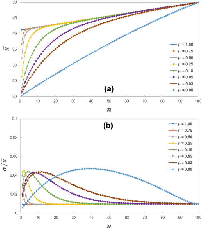
a The dependency of the overall state of compliance \(\bar{\bar{x}}\) on the concurrency of regulatory actions \(n\) and transparency \(\mu\). b The dependency of the noise to signal ratio of the overall state of compliance \(\sigma /\bar{\bar{x}}\) on the concurrency of regulatory actions \(n\) and transparency \(\mu\)
As expected from conventional wisdom, more concurrent regulatory actions or great transparency lead to higher overall state of compliance. The two straight-lines correspond to the cases that no firm has any friend or complete lack of transparency, and each firm reacts to the regulatory actions independently, or all firms are friends to one another or total transparency, and all move together. The use of \(\bar{\bar{x}}\) to represent the overall state of compliance is meaningful in that its noise to signal ratio is generally low, less than 5%, over the entire range of n from 1 to 100, as shown in Fig. 7(b).
The effect of transparency on efficiency can be seen as follows. Take \(n\)=2 in Fig. 7(a), the positive dependency of \(\bar{\bar{x}}\) on \(\mu\) is shown in Fig. 8(a). For instance, an increase of \(\mu\) from 0.25 to 0.75 leads to approximately 33% increase of \(\bar{\bar{x}}\). This result further suggests that increasing transparency is effective in increasing regulatory efficiency.
Fig. 8 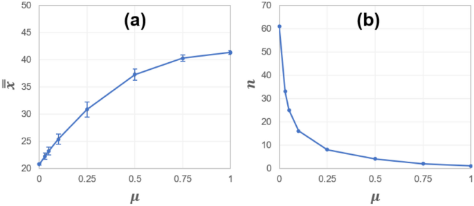
a The dependency of the overall state of compliance \(\bar{\bar{x}}\) on transparency \(\mu\). b The dependency of the concurrency of regulatory actions \(n\) on transparency \(\mu\)
The effect of transparency on cost can be seen as follows. For \(\bar{\bar{x}}\)=40 in Fig. 7(a), the negative dependency of \(n\) on \(\mu\) is shown in Fig. 8(b). For instance, an increase of \(\mu\) from 0.25 to 0.75 leads to a decrease of concurrency from 6 to 2, approximately 67% reduction. If each regulatory action carries the same cost, this translates to a 67% cost reduction. This results further suggest that increasing transparency is effective in saving regulatory cost.
-
(c)
Sequential vs. Concurrent
More regulatory actions lead to higher overall state of compliance, as shown in Figs. 5 and 7, but also higher cost. More regulatory actions can be achieved by increasing their frequency, concurrency or a combination of both. If the cost for each regulatory action is the same, the total cost is proportional to the number of regulatory actions \({n}_{actions}\). Let \({n}_{times}\) denote the number of times that regulatory actions take place during the simulation time \(T\), \({n}_{actions}=n\cdot {n}_{times}\).
A natural question arises as follows. For given \(T\) and \({n}_{actions}\), which approach produces a higher overall compliance, increasing \(n\) and decreasing \({n}_{times}\), or decreasing \(n\) and increasing \({n}_{times}\)? In practical terms, this is equivalent to: for a fixed budget and time, which is more productive, increasing frequency or concurrency? The answer is increasing frequency, as shown in Fig. 9. The setup for this simulation is \(\mu\)=0.5, \(\alpha\)=0.0, and other parameters are listed in Table 2.
Fig. 9 
a The dependency of the overall state of compliance \(\bar{\bar{x}}\) on the concurrency of regulatory actions \(n\). b The dependency of the noise to signal ratio of the overall state of compliance \(\sigma /\bar{\bar{x}}\) on the concurrency of regulatory actions \(n\)
For a given budget \({n}_{actions}\), as concurrency \(n\) increases, the overall state of compliance \(\bar{\bar{x}}\) decreases, as shown in Fig. 9(a). For instance, take \({n}_{actions}\)=300, when \(n\) increases from 1 to 5, \(\bar{\bar{x}}\) decreases from 37 to 29, a drop for nearly 22%. This dependency is true for a moderate budget. For the highest budget of \({n}_{actions}\)=1000 and \(n\)=5, \({n}_{times}\)=200 and \({t}_{interval}\)=50, shorter than \({t}_{elevated}\)=60. Five firms are hit with regulatory actions within the regress-wake cycle time, and nearly all the firms stay compliant at \(\bar{\bar{x}}\approx\)41. For the lowest budget of \({n}_{actions}\)=10 and \(n\)=5, \({n}_{times}\)=2 and \({t}_{interval}\)=5000, much longer than \({t}_{elevated}\)=60. Five firms are hit with regulatory actions approximately every 83 regress-wake cycles, and nearly all the firms stay marginally compliant at \(\bar{\bar{x}}\)=20. The use of \(\bar{\bar{x}}\) to represent the overall state of compliance is meaningful in that its noise to signal ratio is generally low, less than 33%, as shown in Fig. 9(b). For modest concurrency \({n}_{actions}\)=100 to 300, a larger \(n\) tends to lead to a larger noise to signal ratio. For the two extreme cases, where \({n}_{actions}\)=10 and 1000, the ratios are not only low, less than 15% and 2% respectively, but also hardly dependent on \(n\).
These results suggest that for a very large or very small budget, increasing frequency or concurrency of regulatory actions makes little difference, but for a moderate budget, increasing frequency is more productive than increasing concurrency. This is in agreement with conventional wisdom that a steady regulation is better than a loose one with occasional bursts of tightening campaigns.


Effects of Consistency and Transparency
The fundamental question to address here is how consistency affects regulatory effectiveness [33], and the practical questions to address here are: how does consistency affect the overall state of compliance, and how does the answer depend on transparency?
To visualize, consider an illustration simulation run with a similar setup to Fig. 4, except \(\alpha\)=0.5. The trajectories of all 100 firms are shown in Fig. 10, where \(\overline{x}\left(t\right)\) is represented by the black solid curve in the middle, and \(\bar{\bar{x}}\) is represented by the nearby yellow dashed line. The single blue trajectory at the top represents \(x\left(t\right)\) of the firm that received the nearest regulatory action in time, but unlike in Fig. 4, this trajectory no longer stays near \({x}_{fc}\)=50. Instead, it randomly oscillates up and down around 50. A similar up and down pattern is seen from the trajectories of friends.

The regress-wake cycles seen from the time-trajectories of 100 firms in a simulation run with repeated regulatory actions, with inconsistency \(\alpha\)=0.5
The random oscillating trajectories are the result of the inconsistency of regulatory actions and upon receiving a regulatory action, that a firm’s \({k}_{compl}\left(t\right)\) is no longer restored to \({k}_{compl-f}\), but to a random value whose distribution is centered on \({k}_{compl-f}\). Its friends are affected accordingly. The magnitude of oscillation is controlled by \(\alpha\) in Eqs. (7) and (8).
The dependency of the overall state of compliance \(\bar{\bar{x}}\) on inconsistency \(\alpha\) and transparency \(\mu\) is shown in Fig. 11, \(\mathrm{with}\;\mathrm a\;\mathrm{setup}\;\mathrm{of}\;\mathrm T=10,000,\;{\mathrm t}_{\mathrm{interval}}=60\;\mathrm{and}\;\mathrm n=1\). Inconsistency has little impact to the overall state of compliance, as shown in Fig. 11(a), but has significant impact to the standard deviation \(\sigma\). For a given value of \(\alpha\), \(\sigma /\bar{\bar{x}}\) positively depends on \(\mu\). For instance, for \(\alpha\)=0.5, when \(\mu\) increases from 0.25 to 0.75, the noise to signal ratio \(\sigma /\bar{\bar{x}}\) jumps from 7 to 11%, an increase of 57%. This result suggests that transparency has an amplifying effect on inconsistency, in agreement with conventional wisdom that well-publicized ad hoc regulation leads to uneven industry compliance.

a The dependency of the overall state of compliance \(\bar{\bar{x}}\) on inconsistency \(\alpha\) and transparency \(\mu\). b The dependency of the noise to signal ratio of the overall state of compliance \(\sigma /\bar{\bar{x}}\) on inconsistency \(\alpha\) and transparency \(\mu\)
A larger \(\sigma /\bar{\bar{x}}\) indicates \(\bar{\bar{x}}\) is less representative of the overall state of compliance, as there are more firms with higher and lower compliance than \(\bar{\bar{x}}\) at times, the former is fine with the FDA, while the latter is not what the FDA wants to see. In this regard, the quality of regulatory action is adversely impacted by inconsistency.
These results suggest that regulatory consistency is important to achieve high quality outcome from regulatory actions, and the effect of poor consistency is amplified by transparency.
Discussion and Conclusion
Fundamentals of Regulatory Science
The present work proposes proportionality, transparency and consistency as fundamental concepts of regulatory science, improving regulatory effectiveness as a major purpose of regulatory science, and efficiency, cost and quality as basic measures for regulatory effectiveness. By introducing a dynamic model and focusing on the GMP compliance regulation, the present work has established quantitative relationships between the fundamental concepts and the basic measures, and their programmatic implications.
Theoretical Modeling
The state of compliance \(x\left(t\right)\) is proposed as a key variable to characterize a firm’s state of compliance. Its average over an ensemble of firms \(\overline{x}\left(t\right)\) represents the state of compliance of industry. The average of \(\overline{x}\left(t\right)\) over time \(\bar{\bar{x}}\) represents the overall state of compliance. The “\(x\left(t\right)\to \overline{x}\left(t\right)\to\bar{\bar{x}}\)” triplet provides a detailed characterization of the compliance state.
The dynamics of \(x\left(t\right)\) is proposed to follow a generalized Ornstein-Uhlenbeck stochastic equation with a linear constraint force \(-k\left(t\right)\left(x-{x}_{fc}\right)\)derived from a quadratic potential \(U(x,t)\) that represents a myriad of GMP rules. Coefficient \(k\left(t\right)\) represents compliance vigilance and the mechanism of the dynamic model. The “\(x\left(t\right)\to k\left(t\right)\to U(x,t)\)” triplet represents the depth of the theoretical model. Linearity is the model’s built-in feature for proportionality.
The regress-wake cycle is proposed as a key characteristics of the dynamics for both \(x\left(t\right)\) and \(k\left(t\right)\). The regression of \(k\left(t\right)\) is empirically modeled with an exponential function \({e}^{-(t/\tau )}\) for simplicity. The concept of circle of friends is proposed to model the influence among firms, and transparency. A regulatory action is assumed to only affects its receiving firm, which in turn affects its friends. No friend’s impact on friends is included. Moreover, all firms are treated equal, all have the same number of friends and the same influence to friends. These assumptions are not expected to change the main conclusions in present work [34], because the setup of circle of friends is often not perfect, and a mixture of circles of varying sizes has to be used anyway.
The concept of regulatory action in present work is an abstract one, covering GMP inspection, Form 483, Untitled Letter, Import Alert, Warning Letter, and legal actions. Strictly speaking, an inspection is not a regulatory action, but does remind a firm staying vigilant to compliance.
Compliance and quality are related but not the same. The state of compliance is related to but not the same as the state of quality. Moreover, while the state of compliance in present work is a scaler, the dynamic model allows extension to a vector to include, for example, output from the quality metrics and quality management maturity [24,25,26,27]. Vectorization is not expected to qualitatively alter the findings in present work, as long as the constraint force consists of a gradient of \(U(\overrightarrow{x},t)\) and an orthogonal component [35]. Such a component is likely to enrich the model, but is beyond the scope of the present work.
While the dynamic model is based on the fundamental concepts of proportionality, transparency and consistency, it is empirical in nature. Its validation can only come from its agreement with conventional wisdom and its programmatic usefulness. The established relationships between the fundamental concepts and the basic regulatory effectiveness measures, and the programmatic implications can be considered as a partial validation of the model.
Numerical Simulation
A perfect solution for setting up circles of friends so that each firm has the same number of friends may not exist. One can set a target range, and keep looking for a solution, or set the run time of an algorithm and pick the best solution found during the run. The present work uses the latter approach. A better algorithm may find better solutions, but is not expected to produces qualitatively different results.
Given the multi-parameter and multi-variable setup for each simulation, the present work only explored a small portion of all parameter and variable combinations, which are chosen to illustrate certain effects, but are not optimized to do so. In this regard, the present work should be viewed as an illustration of the capabilities of the dynamic model, as opposed to a faithful simulation of real-world situations.
Suggestions to FDA
Policy Suggestion
-
Consider publication of the 483’s together with firms’ responses, or even requiring firms to provide redacted 483’s and responses to improve regulatory transparency.
Operation Suggestion
-
Spread inspections over time, as opposed to making multiple inspections over a short period of time, other considerations notwithstanding, such as inspecting multiple firms during one overseas trip for cost saving.
Quality Management Maturity
-
Associate the quality management maturity with \(\tau\), \({t}_{elevated}\), \({k}_{compl-f}\) and \({k}_{compl-m}\), as in Table 2, the main characteristics of a firm's compliance resilience can be derived from its past compliance record. Doing so enables the encoding of the actual quality management maturity into the dynamics of the compliance state for each individual firm.
-
Expand the concept and practice of circle of friends by experimenting various schemes. For instances, geographical proximity, product similarity and supply-chain dependency can be used to construct a more realistic set of circles of friends.
-
Design optimal algorithms to select firms to inspect in order to achieve maximum impact on the overall compliance state of a chosen set of firms.
-
Compare the simulation results with the actual inspection outcome as a way to validate and improve the dynamic model.
-
Build “a first principle based” data-driven dynamic model to track and to interact with the compliance state for individual firms, for any subset of the firms, or for the entire industry.
The proposed dynamic model allows the FDA use its unique wealth of product and compliance data to build a comprehensive decision-support model to monitor the compliance dynamics of all firms, and use the new data generated from the ongoing compliance operation for model validation and improvement [13]. Such a model may help to address the ultimate questions like: what is the current state of manufacturing quality of the pharmaceutical industry, is it improving or worsening, and how to improve [7]?
The source code of the MATLAB programs used in present work is available to regulatory agencies upon request (zhengqiang@pku.edu.cn).
Data Availability
Not applicable.
Code Availability
Not applicable.
References
US Food and Drug Administration. Current Good Manufacturing Practice (CGMP) Regulations. https://www.fda.gov/drugs/pharmaceutical-quality-resources/current-good-manufacturing-practice-cgmp-regulations. Accessed 07 Feb 2024.
Sutinen JG, Kuperan K. A socio-economic theory of regulatory compliance. Int J Soc Econ. 1999. https://doi.org/10.1108/03068299910229569.
US Food and Drug Administration. What We Do. https://www.fda.gov/about-fda/what-we-do. Accessed 07 Feb 2024.
US Food and Drug Administration. Advancing Regulatory Science. https://www.fda.gov/science-research/science-and-research-special-topics/advancing-regulatory-science. Accessed 07 Feb 2024.
Chiu K, Racz R, Burkhart K, et al. New science, drug regulation, and emergent public health issues: the work of FDA’s division of applied regulatory science. Front Med. 2023. https://doi.org/10.3389/fmed.2022.1109541.
McBride D, Moghissi AA, Steen T, et al. Regulatory Science: the maturation of an Evolving Scientific Discipline. J Regul Sci. 2023. https://doi.org/10.21423/JRS.REGSCI.111272.
US Food and Drug Administration. Report on the State of Pharmaceutical Quality. https://www.fda.gov/about-fda/center-drug-evaluation-and-research-cder/report-state-pharmaceutical-quality. Accessed 07 Feb 2024.
Meyerson D. Why should justice be seen to be done? CRIMINAL JUSTICE ETHICS. 2015. https://doi.org/10.1080/0731129X.2015.1019780.
World Health Organization. Good regulatory practices in the regulation of medical products. 2021. https://www.who.int/publications/m/item/annex-11-trs-1033. Accessed 07 Feb 2024.
Mascini P. Why was the enforcement pyramid so influential? And what price was paid? Regulation & Governance. 2013. https://doi.org/10.1111/rego.12003.
US Food and Drug Administration. Pharmaceutical Quality Documents. https://www.fda.gov/drugs/pharmaceutical-quality-resources/search-pharmaceutical-quality-documents. Accessed 07 Feb 2024.
US Food and Drug Administration. Warning Letters and Notice of Violation Letters to Pharmaceutical Companies. https://www.fda.gov/drugs/enforcement-activities-fda/warning-letters-and-notice-violation-letters-pharmaceutical-companies. Accessed 07 Feb 2024.
US Food and Drug Administration. Understanding CDER’s Risk-Based Site Selection Model. https://www.fda.gov/media/116004/download. Accessed 07 Feb 2024.
US Food and Drug Administration. FDA Form 483. https://www.fda.gov/inspections-compliance-enforcement-and-criminal-investigations/inspection-references/fda-form-483-frequently-asked-questions. Accessed 07 Feb 2024.
US Food and Drug Administration. Regulatory Procedures Manual - Warning Letters. https://www.fda.gov/media/71878/download. Accessed 07 Feb 2024.
Nyborg K, Telle K. The role of warnings in regulation: keeping control with less punishment. J Public Econ. 2004. https://doi.org/10.1016/j.jpubeco.2004.02.004.
Chesney DL. Warning letter: an Enforcement Tool in need of balance. FDLI UPDATE. 2010: 30.
Abdurakhmonov M, Bolton JF, Ridge JW. When the cat’s away, the mice will play: A model of corporate regulatory compliance. J Manag Stud. 2019;7:27.
Anand G, Gray J, Siemsen E. Decay, shock, and renewal: operational routines and process entropy in the pharmaceutical industry. Organ Sci. 2012. https://doi.org/10.1287/orsc.1110.0709.
US Food and Drug Administration. ORA FOIA Electronic Reading Room. https://www.fda.gov/about-fda/office-regulatory-affairs/ora-foia-electronic-reading-room. Accessed 07 Feb 2024.
US Food and Drug Administration. Warning Letters. https://www.fda.gov/inspections-compliance-enforcement-and-criminal-investigations/compliance-actions-and-activities/warning-letters. Accessed 07 Feb 2024.
Hicks PE. Introduction to Industrial Engineering and Management Science. 1st ed. McGraw-Hill; 1977.
Bauschke R. The Effectiveness of European Regulatory Governance: The Case of Pharmaceutical Regulation. 2010.
US Food and Drug Administration. CDER Quality Management Maturity. https://www.fda.gov/drugs/pharmaceutical-quality-resources/cder-quality-management-maturity. Accessed 07 Feb 2024.
Wang G, Wang W, Zheng Q. Quantitative analysis of the QMS for Pharmaceutical Manufacturing. J Pharm Innov. 2021. https://doi.org/10.1007/s12247-021-09579-w.
Fellows M, Friedli T, Li Y, et al. Benchmarking the quality practices of global pharmaceutical manufacturing to advance supply chain resilience. AAPS J. 2022. https://doi.org/10.1208/s12248-022-00761-7.
Maguire J, Fisher A, Harouaka D, et al. Lessons from CDER’s Quality Management Maturity Pilot Programs. AAPS J. 2023. https://doi.org/10.1208/s12248-022-00777-z.
Uhlenbeck GE, Ornstein LS. On the theory of the Brownian motion. Phys Rev. 1930;36(5):823.
Blackwell PG. Ornstein-Uhlenbeck process: Overview. Wiley StatsRef: Statistics Reference Online. 2014. https://doi.org/10.1002/9781118445112.stat05077.
Thornton D, Gunningham NA, Kagan RA. General deterrence and corporate environmental behavior. LAW POLICY. 2005. https://doi.org/10.1111/j.1467-9930.2005.00200.x.
Erdős P, Rényi A. On the evolution of random graphs. PUBLICATION Math Inst Hung Acad Sci. 1960;5(1):17–60.
US Government Accountability Office. COVID-19 Complicates Already Challenged FDA Foreign Inspection Program. https://www.gao.gov/assets/gao-20-626t.pdf. Accessed 07 Feb 2024.
Shiihi S, Okafor UG, Ekeocha Z et al. Improving the outcome of GMP inspections by improving proficiency of inspectors through consistent GMP trainings. BIRS Africa Technical Report Papers. 2021. https://doi.org/10.5703/1288284317433.
Wu AA, Wang YI. The more monitoring, the better quality? Empirical evidence from the generic drug industry. Empir Evid Generic Drug Ind. 2021. https://doi.org/10.2139/ssrn.3596559.
Zheng Q, Hao B. Steady state solutions of the Fokker-Planck equations. Commun Theor Phys. 1987. https://doi.org/10.1088/0253-6102/8/2/153.
Acknowledgements
The authors thank Guoxu Wang, Liang Han, Garth Boehm and Joseph Famulare for helpful discussions and suggestions, and PKU-Hisun QbD Lab, PKU-Siyao GMP Lab, PKU-Hepalink Research Fund, PKU-Merck Serono Research Fund, and PKU-MSD Research Fund for support.
Funding
PKU-Hisun QbD Lab, PKU-Siyao GMP Lab, PKU-Hepalink Research Fund, PKU-Merck Serono Research Fund, and PKU-MSD Research Fund. PKU (Peking University).
Author information
Authors and Affiliations
Contributions
Not applicable.
Corresponding author
Ethics declarations
Ethics Approval
Not applicable.
Consent to Participate
Not applicable.
Consent for Publication
Not applicable.
Conflict Interests
Not applicable.
Additional information
Publisher’s Note
Springer Nature remains neutral with regard to jurisdictional claims in published maps and institutional affiliations.
Rights and permissions
Open Access This article is licensed under a Creative Commons Attribution 4.0 International License, which permits use, sharing, adaptation, distribution and reproduction in any medium or format, as long as you give appropriate credit to the original author(s) and the source, provide a link to the Creative Commons licence, and indicate if changes were made. The images or other third party material in this article are included in the article's Creative Commons licence, unless indicated otherwise in a credit line to the material. If material is not included in the article's Creative Commons licence and your intended use is not permitted by statutory regulation or exceeds the permitted use, you will need to obtain permission directly from the copyright holder. To view a copy of this licence, visit http://creativecommons.org/licenses/by/4.0/.
About this article

Cite this article
Bao, Y., Buhay, N. & Zheng, Q. A Dynamic Model for GMP Compliance and Regulatory Science. J Pharm Innov 19, 25 (2024). https://doi.org/10.1007/s12247-024-09825-x
Accepted:
Published:
DOI: https://doi.org/10.1007/s12247-024-09825-x