Attacking the linear congruential generator on elliptic curves via lattice techniques

Abstract

In this paper we study the linear congruential generator on elliptic curves from the cryptographic point of view. We show that if sufficiently many of the most significant bits of the composer and of three consecutive values of the sequence are given, then one can recover the seed and the composer (even in the case where the elliptic curve is private). The results are based on lattice reduction techniques and improve some recent approaches of the same security problem. We also estimate limits of some heuristic approaches, which still remain much weaker than those known for nonlinear congruential generators. Several examples are tested using implementations of ours algorithms.

1 Introduction

A PseudoRandom Bit Generator(PRBG) is a deterministic algorithm that, once initialized with some random value (called the seed), outputs a sequence that appears random, in the sense that an observer who does not know the value of the seed cannot distinguish the output from that of a (true) random bit generator. PRBG’s have important applications on simulations (e.g. for the Monte Carlo method), electronic games (e.g. for procedural generation), and cryptography. Good statistical properties are a vital requirement for the output of a PRBG. Cryptographic applications require the output not to be predictable from earlier outputs, and more elaborate algorithms, which do not inherit the linearity of simpler PRBGs, are needed.

There is a vast literature devoted to generating pseudorandom numbers using arithmetic of finite field and residue rings, see [33, 37, 38, 45]. In 1994, Hallgreen [21] proposed a pseudorandom number generator based on the group of points of an elliptic curve defined over a prime finite field.

For a prime p, denote by $\mathbb {F}_{p}$ the field of p elements and always assume that it is represented by the set {0,1,…,p − 1}. Accordingly, sometimes, where obvious, we treat elements of $\mathbb {F}_{p}$ as integer numbers in the above range.

Let E be an elliptic curve defined over $\mathbb {F}_{p}$ given by an affine Weierstrass equation, which for $\gcd (p,6)=1$ takes form

$$ Y^{2}=X^{3}+aX+b, $$

(1)

for some $a,b \in \mathbb {F}_{p}$ with 4a³ + 27b²≠ 0.

We recall that the set $E(\mathbb {F}_{p})$ of $\mathbb {F}_{p}$-rational points forms an abelian group, with the point at infinity $\mathcal {O}$ as the neutral element of this group (which does not have affine coordinates).

For a given point $G \in E(\mathbb {F}_{p})$ the Linear Congruential Generator on Elliptic Curves, EC-LCG is a sequence U_n of pseudorandom numbers defined by the relation

$$ U_{n}=U_{n-1}\oplus G=nG\oplus U_{0}, \quad n=1,2,\ldots, $$

(2)

where ⊕ denotes the group operation in $E(\mathbb {F}_{p})$ and $U_{0} \in E(\mathbb {F}_{p})$ is the initial value or seed. We refer to G as the composer of the EC-LCG.

It is clear that the period of the sequence (2) is equal to the order of G. The EC-LCG provides a very attractive alternative to linear and non-linear congruential generators with many applications to cryptography and it has been extensively studied in the literature, see [3, 12, 17, 18, 21, 22, 34, 35, 39, 40].

In the cryptographic setting, the initial value U₀ = (x₀,y₀) and the constants G, a, and b are assumed to be the secret key, and we want to use the output of the generator as ephemeral key of a stream cipher. Of course, if two consecutive values U_n are revealed, it is almost always easy to find U₀ and G. So, we output only the most significant bits of each U_n in the hope that this makes the resulting output sequence difficult to predict.

It is known that not too many bits can be output at each stage: the EC-LCG is unfortunately predictable if sufficiently many bits of its consecutive elements are revealed, see [20, 31, 32].

Now, we are formalising the results. Assume that the sequence (U_n) is not known, but for some n, approximations W_j of two consecutive values U_n+j, j = 0,1 are given. The results involve another parameter Δ which measures how well the values W_j approximate the terms U_n+j. This parameter is assumed to vary independently of p subject to satisfying the inequality Δ < p (and is not involved in the complexity estimates of our algorithms). More precisely, we say that $W=(x_{W},y_{W}){\in {\mathbb {F}}_{p}^{2}}$ is a Δ-approximation to $U=(x_{U},y_{U}){\in \mathbb {F}_{p}^{2}}$ if there exist integers e,f satisfying:

$$|e|,|f|\leq{\Delta},\ x_{W}+ e=x_{U},\ y_{W}+ f=y_{U}.$$

In general, we say that $W=(\alpha _{1},\alpha _{2},\ldots ,\alpha _{n}) {\in \mathbb {F}_{p}^{n}}$ is a Δ-approximation to $U=(x_{1},x_{2},\ldots ,x_{n}) {\in \mathbb {F}_{p}^{n}}$ if there exist integers 𝜖_i, (i = 1,…,n) satisfying:

$$|\epsilon_{i}| \leq{\Delta},\ \alpha_{i}+ \epsilon_{i}=x_{i}, \quad i=1,\ldots,n.$$

The case where Δ grows like a fixed power p^δ where 0 < δ < 1 corresponds to the situation where a positive proportion δ of the least significant bits of terms of the output sequence remain hidden. The goal is to get δ as much larger as possible, recovering the rest of the bits in polynomial time.

The problem is a particular case of the following computational problem: given f₁(X₁,…,X_n),…,f_s(X₁,…,X_n) irreducible multivariate polynomials defined over the integer ring ${\mathbb {Z}}$, having a common root (x₁,…,x_n) modulo a known integer N, namely,

$$f_{i}(x_{1},\ldots,x_{n}) \equiv 0 \bmod N, \quad i=1,\ldots,s.$$

The root should be small root, in the sense that each x_i is bounded by a known value Δ. We require to bound the sizes of Δ allowing to recover the desired root in polynomial time. For polynomial in one variable an algorithm has been given by Coppersmith in [9]. For bivariate polynomials does exist different methods in [6, 10, 11, 16] and, for general multivariate polynomials in [16, 24]. All of them are based on the so called lattice reduction techniques, also called the LLL techniques, because the celebrated LLL algorithm of Lenstra, Lenstra and Lovász [30]. However in the general case only heuristic results are known, which are just generalization of the original result by Coppersmith.

An algorithm to recover the seed U₀ in deterministic polynomial time if Δ < p^1/6, requiring compute a closest vector of a lattice of dimension 8 and coefficients size $\log p$ is presented in [20]. The recent results [31, 32] recover ‘heuristically’ the seed U₀ if Δ < p^1/5. The heuristic method, since there is no guarantee of success, may fail by several reason, among them the difficulty of finding a short vector in a high dimensional lattice. Since the number of the monomials is quite large; those results does not imply practical attacks, since the naive application of Coppersmith method is impractical for high dimensional lattice.

The computation which is theoretically polynomial-time becomes in practice prohibitive, for instance and according to [32], if the quality is 0.187 < 0.2 = 1/5 requires 188 polynomials and 314 monomials, so the lattice dimension is 502.

In this paper, we prove a deterministic algorithm to recover the seed U₀ in polynomial time if Δ < p^1/6, requiring compute a closest vector of a lattice of dimension 5. Previous result in [20] required a lattice of dimension 8.

We also provide an heuristic method to recovering U₀ if ${\Delta } < p^{\frac {k-1}{4k-2}}$, requiring compute a closest vector for a lattice of dimension 3k − 1, when k > 2 consecutive Δ −approximations to points U_i, (0,…,k − 1) of the curve E are given. A similar result is also presented in [31, 32] with a theoretical better bound ${\Delta } < p^{\frac {3k}{11k+4}}$, but again requiring computing LLL’s algorithm for a lattice of huge dimension. In fact, there is no practical way of testing their methods, not only because the lattice large dimension used, but the size of the prime p should be several hundreds of bits. On the other hand, for instance, we can recover the sequence produced by EC-LCG if only three consecutive Δ −approximations are given as soon as Δ < p^1/5 requiring, the most time consuming, to find a closest vector for a lattice of dimension 7, and it matched by primes p of only 1000 bits.

In principle, we cannot obtain any approximation to composer G from any approximations to two consecutive values U_n,U_n+ 1 of the EC-LCG, because the elliptic curve group operation. We also rigorously demonstrate our approach in the special case when we have an approximation to composer G; we show that given Δ if sufficiently many of the most significant bits of G and of three consecutive values U_n,U_n+ 1,U_n+ 2 of the EC-LCG are given, one can recover the seed U₀ and the composer G as soon as O(Δ) < p^1/6 requiring compute two closest vector for two lattices of dimension 7. And heuristic algorithm if O(Δ) < p^5/12 by computing a short vector for a lattice of dimension 9. Finally, we obtain an heuristic method to recovering the whole sequence if ${\Delta } < p^{\frac {k-1}{5k-4}}$, by computing a closest vector of a certain lattice of dimension 4k − 3 when k > 2 consecutive Δ −approximations to points U_i, (0,…,k − 1) of the curve E and an Δ −approximation to composer G are given.

This suggests that for cryptographic applications EC-LCG should be used with great care. For the linear congruential generator similar problems have been introduced by Knuth [26] and then considered in [7, 13, 23, 27]; see also the surveys [8, 28]. The quadratic congruential generator and the inverse congruential generator have been studied in [4] and [15], see also the recent paper [44] for a more general problem

On the other hand, our results are substantially weaker than those known for the linear and nonlinear congruential generators.

The remainder of the paper is structured as follows. We start with a very short outline of some basic facts about the Closest Vector Problem (CVP), and the polynomial equations associated to the elliptic curve abelian group in Section 2. In Section 3 we attack the EC-LCG when the composer G is known. Section 4 is dedicated to study the case when the composer G is private. Then in Section 5 we discuss the results of numerical tests of pour approaches. We conclude with Section 6, which makes some final comments and poses open questions.

Throughout the paper, we use the convention that the parameters on which the implied constant in a Landau symbol O are written in the subscript of O. A symbol O without a subscript indicates and absolute implied constant.

2 Preliminaries

2.1 Closest vector problem in lattices

Here we review some results and definitions concerning the Closest Vector Problem, all of which can be found in [19]. For more details and more recent references, we recommend consulting [23].

Let {b₁,…,b_s} be a set of linearly independent vectors in ${\mathbb {R}}^{r}$. The set

$$ \mathcal{L}=\{c_{1}\textbf{b}_{1}+\cdots+ c_{s}\textbf{b}_{s}\ |\ c_{1}, \ldots, c_{s}\in\mathbb{Z}\} $$

is an s-dimensional lattice with basis {b₁,…,b_s}. If s = r, the lattice ${\mathscr{L}}$ is of full rank.

One basic lattice problem is the Closest Vector Problem (CVP): given a basis of a lattice ${\mathscr{L}}$ in $\mathbb {R}^{s}$ and a shift vector t in $\mathbb {R}^{s}$, the goal is finding a vector in the lattice ${{\mathscr{L}}}$ closest to the target vector t. It is well known that this problem is NP-hard when the dimension grows. However, it is solvable in deterministic polynomial time provided that the dimension of ${{\mathscr{L}}}$ is fixed (see [25], for example).

In fact, lattices in this paper consist of integer solutions:

$\textbf x=(x_{0},\ldots ,x_{s-1})\in ~\mathbb {Z}^{s}$ of a system of congruences

$$ \sum\limits_{i=0}^{s-1} a_{ij} x_{i} \equiv 0 \bmod {q_{j}}, \qquad j = 1, \ldots, m, $$

modulo some positive integers q₁,…,q_m. Typically (although not always) the volume of such a lattice is the product Q = q₁⋯q_m. Moreover, all the aforementioned algorithms, when applied to such a lattice, become polynomial in $\log Q$. If textbfb₁,…,b_s} is a basis of the above lattice, by the Hadamard inequality we have:

$$ \prod\limits_{i=1}^{s} \|\textbf{b}_{i}\|\geq\text{vol}({\mathcal{L}}). $$

(3)

For a slightly weaker task of finding a sufficiently close vector, the celebrated LLL algorithm of Lenstra, Lenstra and Lovász [30] provides a desirable solution, as noticed by [2], that is, a polynomial time algorithm in the bit size coefficients of the lattice basis and also of the lattice dimension. Here, we state this result as Lemma 1.

Lemma 1

There exists a deterministic polynomial time algorithm which, when given an s-dimensional full rank lattice ${\mathscr{L}}$ and a shift vector t, finds a lattice vector $\textbf {u}\in {\mathscr{L}}$ satisfying the inequality

$$ \|\textbf{t}-\textbf{u}\|\le 2^{s/2}\min\{\|\textbf{t}-\textbf{v}\|:\ \textbf{v}\in\mathcal{L}\}. $$

An outline of the algorithms presented in this paper goes as follows. They are divided into two stages.

• Stage 1: We construct a certain lattice ${{\mathscr{L}}}$ of dimension s; this lattice depends on the given approximations. We also show that a certain vector E directly related to missing information is a very short vector. A closest vector F is found; see [25] for fixed dimension and Lemma 1 the approximation solution for arbitrary dimension.

• Stage 2: We show that F provides the required information about E if the approximation is good enough.

Many other results on both exact and approximate finding of a closest vector in a lattice are discussed in [19, 23].

2.2 The polynomial equation of the group associated to an elliptic curve

The operation ⊕ acts over the points P = (x_P,y_P) and Q = (x_Q,y_Q) of $E(\mathbb {F}_{p})$ with $P, Q \not = \mathcal {O}$ as follows:

$$P \oplus Q =R=(x_{R},y_{R})$$

• If x_P≠x_Q, then

  $$ \begin{array}{cc} x_{R}=m^{2}-x_{P}-x_{Q}, \qquad &y_{R}=m(x_{P}-x_{R})-y_{P}, \\ &\text{~where}\qquad m =\frac{y_{Q}-y_{P}}{x_{Q}-x_{P}}. \end{array} $$

  (4)

• If x_P = x_Q but y_P≠y_Q, then $P \oplus Q =\mathcal {O}$.

• If P = Q and y_P≠ 0, then

  $$ \begin{array}{ll} x_{R}=m^{2}-2x_{P}, \qquad &y_{R}=m(x_{P}-x_{R})-y_{P}, \\ &~~\text{where}\quad m =\frac{3{x_{P}^{2}}+a}{2y_{P}}. \end{array} $$

  (5)

• If P = Q and y_P = 0, then $P \oplus Q =\mathcal {O}$.

See [1, 5, 43] for these and other general properties of elliptic curves.

Our context is a pseudorandom bit generator which outputs affine points in an elliptic curve. One obtains recursively them by operating a fixed composer G to the previous value. So, almost always, the above equations in the first case (4) will determine the process.

If P is not Q or − Q, then, clearing denominators in (4), we can translate P ⊕ Q = R into the following identities in the field $\mathbb {F}_{p}$:

$$L_{1}=L_{1}(x_{Q},y_{Q},x_{P},y_{P},x_{R})\equiv 0 \bmod p$$

and

$$L_{2}=L_{2}(x_{Q},y_{Q}, x_{P},y_{P},x_{R},y_{R}) \equiv 0 \bmod p,$$

where

$$ \begin{array}{ll} L_{1}={x_{{Q}}}^{3}+x_{{R}}{x_{{Q}}}^{2}-x_{{P}}{x_{{Q}}}^{2}-2 x_{{R}}x_{{ Q}}x_{{P}}-x_{{Q}}{x_{{P}}}^{2}\\+{x_{{P}}}^{3}+2y_{{Q}}y_{{P}}+x_{{R} }{x_{{P}}}^{2}-{y_{{Q}}}^{2}-{y_{{P}}}^{2}, \\ L_{2}= y_{{R}}x_{{Q}}-y_{{R}}x_{{P}}-y_{{Q}}x_{{P}}+y_{{Q}}x_{{R}}-y_{{P}}x_{ {R}}+y_{{P}}x_{{Q}}. \end{array} $$

(6)

Lemma 2

Let L₁(X_Q,Y_Q,X_P,Y_P,X_R),L₂(X_Q,Y_Q,X_P,Y_P,X_R,Y_R) be elements of the polynomial ring $\mathbb {F}_{p}[X_{Q},Y_{Q},X_{P},Y_{P},X_{R},Y_{R}]$ and let U,V,W be algebraically independent variables.

• 1. Let Φ be the linear transformation:

  $$(X_{P} \to X_{P}, Y_{P}\to Y_{P}, X_{Q}\to X_{P}+U, Y_{Q} \to Y_{P} +V, X_{R} \to X_{P} +W)$$

  we have Φ(L₁) = 3X_PU² + U³ + U²W − V².

• 2.
  $$ L_{1}(X_{Q},Y_{Q}+U,X_{P}, Y_{P}+U, X_{R}) = L_{1}(X_{Q},Y_{Q},X_{P},Y_{P},X_{R})$$
  $$ L_{2}(X_{Q}+U,Y_{Q},X_{P}+U, Y_{P}, X_{R}+U, Y_{R}) = L_{2}(X_{Q},Y_{Q},X_{P},Y_{P},X_{R},Y_{R})$$

Proof

It is straightforward. □

On the other hand, since P = (x_P,y_P), Q = (x_Q,y_Q) and R = (x_R,y_R) are points of the elliptic curve E, we have:

$$ \begin{array}{ll} {y_{P}^{2}}={x_{P}^{3}}+ax_{P}+b, \\ {y_{Q}^{2}}={x_{Q}^{3}}+ax_{Q}+b, \\ {y_{R}^{2}}={x_{R}^{3}}+ax_{R}+b. \end{array} $$

Eliminating the curve parameters a, b and assuming that x_P≠x_R, we obtain the following polynomial $L_{3} \in \mathbb {F}_{p}[X_{Q},Y_{Q},X_{P},Y_{P},X_{R},Y_{R}]$

$$ \begin{array}{ll} L_{3}=- {X_{R}^{3}} X_{P} + {X_{R}^{3}} X_{Q} + X_{R} {X_{P}^{3}} - X_{R} {Y_{P}^{2}} - X_{R} {X_{Q}^{3}} + X_{R} {Y_{Q}^{2}} \\+ {Y_{R}^{2}} X_{P} - {Y_{R}^{2}} X_{Q} - {X_{P}^{3}} X_{Q} + X_{P} {X_{Q}^{3}} - X_{P} {Y_{Q}^{2}} + {Y_{P}^{2}} X_{Q} \end{array} $$

(7)

verifying L₃(x_Q,y_Q,x_P,y_Q,x_R,y_R) ≡ 0 mod p. Now, we consider the linear map Θ :

$$(X_{Q} \to X_{Q}, Y_{Q}\to Y_{P}+U, X_{P}\to X_{P}, Y_{P} \to Y_{P}, X_{R} \to X_{R}, Y_{R}\to -Y_{P}+V)$$

$$ \begin{array}{ll} {\Theta}(L_{3})= [2U(X_{Q}-X_{P})+2V(X_{R}-X_{P})]Y_{P}+A \end{array} $$

(8)

where degree of $A\in \mathbb {F}_{p}[X_{Q},Y_{Q},X_{P},Y_{P},X_{R},Y_{R}, U,V]$ with respect the variable Y_P is zero.

3 Predicting EC-LCG for Known composer

Assume that a, b are unknown, but the prime p is given to us. In [20] shows that when we are given Δ-approximations W_n, W_n+ 1 to (respectively) two consecutive affine values U_n, U_n+ 1 produced by the EC-LCG; we can recover the exact values, provided that x₀ does not lie in a certain set, whose size is bounded by O(Δ⁶). Note that once two affine points in a curve as (1) are given, such that their first component is different, the curve (the parameters a and b) are determined. Then, after discovering the values U_n and U_n+ 1, we can reproduce (backwards and forwards) the whole sequence. To simplify the notation, we assume that n = 0 from now on.

We write W_j = (α_j,β_j), U_j = (x_j,y_j), for j = 0,1; so there exist integers e_j, f_j for j = 0, 1 with:

$$ \begin{array}{ll} x_{j}=\alpha_{j}+{e_{j}},\quad y_{j}={\upbeta}_{j}+ {f_{j}}\\ |e_{j}|, |f_{j}| \le {\Delta}, \quad j=0, 1. \end{array} $$

(9)

Theorem 1

[20] With the above notations and definitions, there exists a set $\mathcal {U}({\Delta };a,x_{G},$ $y_{G})\subseteq \mathbb {F}_{p}$ of cardinality $\# \mathcal {U}({\Delta };a,x_{G},y_{G}) = O({\Delta }^{6})$ with the following property: whenever $x_{0} \not \in \mathcal {U} ({\Delta };a,x_{G},y_{G})$ then, given Δ −approximations W₀, W₁ to two consecutive affine values U₀,U₁ produced by linear congruential generator on elliptic curves (2), and given the prime p one can recover the seed U₀ in deterministic polynomial time.

The proof of this result in [20], the ‘bad’ set of values $\mathcal {U}({\Delta };a,x_{G},y_{G})$ for the components x₀ is described, proving whenever that value lies outside the set, the algorithm works correctly. Furthermore, the size of the set is asymptotically bounded with Δ⁶. This means that if Δ = o(p^1/6) and p is large enough, assuming an uniform distribution of probabilities for $x_{0} \in {\mathbb {F}}_{p}$, the method is unlikely to fail.

The proof in [20] requires the two polynomials L₁ and L₂ of (6) and 8 monomials, so the involved lattice has dimension 8. Here, we use only the polynomial L₂ of (6), then the corresponding lattice dimension is only 5. The present proof is a simple observation of the same strategy, we have included here a significant part of the details for the reader convenience.

Proof

We assume that $x_{0} \in \mathbb {F}_{p}$ is chosen so as not to lie in a certain subset $\mathcal {U}({\Delta };a,x_{G},y_{G})$ of $\mathbb {F}_{p}$ We place the value $x_{G}\in \mathcal {U}({\Delta };a,x_{G},y_{G})$, so that U₀ is not G or − G. Then, clearing denominators in (4),

$$ U_{1}=U_{0}\oplus G $$

(10)

we obtain

$$L_{2}(x_{G},y_{G}, x_{0},y_{0},x_{1},y_{1}) \equiv 0 \bmod p,$$

Using the equalities x_j = α_j + e_j and y_j = β_j + f_j for j = 0,1, the polynomial L₂ of (6) become:

$\left (-{\upbeta }_{1}-y_{G}\right )e_{0}+\left (x_{G}-\alpha _{1}\right )f_{0}+\left (y_{G}-{\upbeta }_{0}\right )e_{1}+\left (x_{G}-\alpha _{0}\right )f_{1}-[e_{0}f_{1}+e_{1}f_{0}] =$

$${\upbeta}_{1}\alpha_{0}-x_{G}{\upbeta}_{1}+y_{G}\alpha_{0}-y_{G}\alpha_{1}+{\upbeta}_{0}\alpha_{1}-x_{G}{\upbeta}_{0}.$$

Now, we linearize this polynomial system. Writing

$$ \begin{array}{ll} B_{0} \equiv {\upbeta}_{1}\alpha_{0}-x_{G}{\upbeta}_{1}+y_{G}\alpha_{0}-y_{G}\alpha_{1}+{\upbeta}_{0}\alpha_{1}-x_{G}{\upbeta}_{0} \bmod p,\\ B_{1} \equiv -{\upbeta}_{{1}}-y_{{G}} \bmod p, \quad B_{2} \equiv x_{{G}}-\alpha_{{1}} \bmod p, \\ B_{3} \equiv y_{{G}}-{\upbeta}_{{0}} \bmod p, \quad B_{4} \equiv x_{{G}}-\alpha_{{0}} \bmod p, \\ B_{5} \equiv -1 \bmod p. \end{array} $$

(11)

is it easy to check that the vector

$$E=({\Delta} e_{0}, {\Delta} f_{0}, {\Delta} e_{1}, {\Delta} f_{1}, e_{1}f_{0}+e_{0}f_{1})=$$

$$({\Delta} E_{1}, {\Delta} E_{2}, {\Delta} E_{3}, {\Delta} E_{4}, E_{5})$$

is a solution to the following linear system of congruences:

$$ \begin{array}{ll} {\sum}_{i = 1}^{4} B_{i}X_{i} + {\Delta} B_{5} \equiv {\Delta} B_{0} \bmod p, \\ X_{1} \equiv X_{2} \equiv X_{3} \equiv X_{4} & \equiv 0 \bmod {\Delta} \end{array} $$

(12)

Moreover, bounds (9) implies E is a relatively short vector. We have:

$$ |E_{i}|\le{\Delta},i=1,2,3,4, \ |E_{5}|\le2{\Delta}^{2};\ \|\textbf E\|\leq\sqrt{8}{\Delta}^{2}. $$

(13)

Let ${{\mathscr{L}}}$ be the lattice consisting of integer solutions $\textbf {X}=(X_{1},X_{2},\ldots ,X_{5})\in {\mathbb {Z}}^{5}$ of the system of congruences:

$$ \begin{array}{@{}rcl@{}} \sum\limits_{i = 1}^{4} B_{i}X_{i} +B_{5}X_{5} \equiv 0 \bmod p, \\ X_{1} \equiv X_{2} \equiv X_{3} \equiv X_{4} & \equiv 0 \bmod {\Delta}. \end{array} $$

(14)

We compute a solution T of the system of congruences (12), using linear diophantine equations methods. Applying an algorithm solving the CVP for the shift vector T and the lattice (14), we obtain a vector

$$\textbf F = ({\Delta} F_{1}, {\Delta} F_{2}, {\Delta} F_{3}, {\Delta} F_{4}, F_{5}).$$

We have F = v + T (where v is the lattice vector returned by the CVP algorithm) is the vector of minimal norm satisfying (12), hence F must have norm at most equal to the norm of the solution E. Using the bounds (13), we get:

$$ \| \textbf F \| \le \sqrt{8}{\Delta}^{2}. $$

(15)

Note that we can compute F in polynomial time from the information we are given. We might hope that E and F are the same, or at least, that we can recover the approximations errors from F. If not, we will show that x₀ belongs to a subset $\mathcal {U}({\Delta };a,x_{G},y_{G}) \subseteq \mathbb {F}_{p}$ of cardinality $\# \mathcal {U}({\Delta };a,x_{G},y_{G}) = O({\Delta }^{6})$. Vector D = E −F lies in ${{\mathscr{L}}}$:

$$\textbf D = ({\Delta} D_{1}, {\Delta} D_{2}, {\Delta} D_{3}, {\Delta} D_{4}, D_{5}), \quad D_{i}=E_{i}-F_{i}, i=1,\ldots, 5. $$

Bounds (13) and (15) imply ∥D∥≤ 4Δ² and

$$ |D_{i}| \le 4{\Delta}, i=1,2,3,4, \quad |D_{5}| \le 4{\Delta}^{2}. $$

From here, by closely following the proof in [20], since only depends on L₂ and D_i, we bound the “bad” possibilities for which this process does not succeed. □

We now present some heuristic arguments showing that Theorem 1 could possibly be strengthened so that it becomes nontrivial when the precision Δ is of the order of p^1/4 rather than of order p^1/6 as currently.

The heuristic that we use is of a totally different nature than that used in the so called Coppersmith’s method, where the heuristic assumption is that all created polynomials define a zero dimension algebraic variety. Here, we use the so-called “Gaussian heuristic” that suggests that and s-dimensional lattice ${\mathscr{L}}$ with volume $vol({\mathscr{L}})$ is unlikely to have a nonzero vector which is substantially shorter than $vol({\mathscr{L}})^{1/s}$. Moreover, if it is known that such a very short vector does exist, then up to a scalar factor it is likely to be the only vector with this property.

Let us formalise the problem. Again, we assume that a, b are unknown, but the prime p is given to us. Suppose that we are given k ≥ 2 consecutive Δ −approximations W_j = (α_j,β_j) to $U_{j} =(x_{j},y_{j}) \in E({\mathbb {F}}_{p})$ (j = 0,…,k − 1), produced by the EC-LCG, so there exist integers e_j, f_j with:

$$ \begin{array}{ll} x_{j}=\alpha_{j}+{e_{j}},\quad y_{j}={\upbeta}_{j}+ {f_{j}}\\ |e_{j}|, |f_{j}| \le {\Delta}, \quad j=0, \ldots,k-1 \end{array} $$

(16)

Theorem 2

With above notation, under the ‘Gaussian heuristic’ we can recovering the seed U₀ in polynomial time in $\log p$ as soon as ${\Delta } < p^{\frac {k-1}{4k-2}}$ by computing a closest vector of a certain lattice of dimension 3k − 1.

Proof

As in the previous Theorem 1 we use only the polynomial L₂ in (6) for a pair of points (U_j,U_j+ 1) for j = 0,…,k − 2. Again, we translate U_j+ 1 = U_j ⊕ G into a polynomial system of equation:

$$ \begin{array}{ll} L^{(0)}_{2}(x_{G},y_{G}, x_{0},y_{0},x_{1},y_{1}) =L_{2}(x_{G},y_{G}, x_{0},y_{0},x_{1},y_{1}) \equiv 0 \bmod p,\\ L^{(1)}_{2}(x_{G},y_{G}, x_{1},y_{1},x_{2},y_{2})=L_{2}(x_{G},y_{G}, x_{1},y_{1},x_{2},y_{2}) \equiv 0 \bmod p,\\ {\cdots} \\ {\cdots} \\ L^{(k-2)}_{2}(x_{G},y_{G}, x_{k-2},y_{k-2},x_{k-1},y_{k-1}) = L_{2}(x_{G},y_{G}, x_{k-2},y_{k-2},x_{k-1},y_{k-1}) \!\equiv\! 0 \bmod p. \end{array} $$

Using the equalities (16) the above polynomial $L^{(j)}_{2}$, for j = 0,…,k − 2, becomes:

$\left (-{\upbeta }_{j+1}-y_{G}\right )e_{j}+\left (x_{G}-\alpha _{j+1}\right )f_{j}+\left (y_{G}-{\upbeta }_{j}\right )e_{j+1}+\left (x_{G}-\alpha _{j}\right )f_{j+1}-[e_{j}f_{j+1}+e_{j+1}f_{j}] =$

$${\upbeta}_{j+1}\alpha_{j}-x_{G}{\upbeta}_{j+1}+y_{G}\alpha_{j}-y_{G}\alpha_{j+1}+{\upbeta}_{j}\alpha_{j+1}-x_{G}{\upbeta}_{j}.$$

Now, we linearize this polynomial system. Writing, for j = 0,…,k − 2 and for i = 0,…,k − 1:

$$ \begin{array}{ll} {\Sigma}^{(j)} \equiv {\upbeta}_{j+1}\alpha_{j}-x_{G}{\upbeta}_{j+1}+y_{G}\alpha_{j}-y_{G}\alpha_{j+1}+{\upbeta}_{j}\alpha_{j+1}-x_{G}{\upbeta}_{j} \bmod p, \\ A^{(j)}_{j} \equiv -{\upbeta}_{j+1}-y_{G} \bmod p, A^{(j)}_{j+1} \equiv y_{{G}}-{\upbeta}_{{j}} \bmod p, \\ B^{(j)}_{j+1} \equiv x_{G}-\alpha_{j+1} \bmod p, B^{(j)}_{j} \equiv x_{{G}}-\alpha_{{j}} \bmod p, \\ A^{(j)}_{i} \equiv 0 \bmod p, B^{(j)}_{i} \equiv 0 \bmod p, \quad i \not=j \lor i \not=j+1,\\ C^{(j)}_{j} \equiv -1 \bmod p, C^{(j)}_{i} \equiv 0 \bmod p, j\not=i. \end{array} $$

we obtain that vector E =

$$({\Delta} e_{0}, {\Delta} e_{1},\ldots, {\Delta} e_{k-1}, {\Delta} f_{0}, {\Delta} f_{1},\ldots, {\Delta} f_{k-1},$$

$$ e_{1}f_{0}+e_{0}f_{1}, e_{2}f_{1}+e_{1}f_{2}, \ldots, e_{k-1}f_{k-2}+e_{k-2}f_{k-1})$$

$$=({\Delta} E_{1}, \ldots, {\Delta} E_{k}, {\Delta} E_{k+1}, \ldots, {\Delta} E_{2k},E_{2k+1}, \ldots,E_{3k-1})$$

is a solution to the following linear system of congruences (j = 0,…,k − 2):

$$ \begin{array}{ll} {\sum}_{i = 0}^{k-1} A^{(j)}_{i}X_{i} +{\sum}_{i = 0}^{k-1} B^{(j)}_{i}Y_{i} + {\sum}_{i=0}^{k-1}{\Delta} C^{(j)}_{i}Z_{i} \equiv {\Delta} {\Sigma}^{j} \bmod p, \\ X_{0} \equiv X_{1} \equiv {\ldots} \equiv X_{k-1} & \equiv 0 \bmod {\Delta} \\ Y_{0} \equiv Y_{1} \equiv {\ldots} \equiv Y_{k-1} & \equiv 0 \bmod {\Delta}. \end{array} $$

(17)

Moreover, bounds (16) imply E is a relatively short vector. We have:

$$ \|\textbf E\|\leq\sqrt{6k-6}{\Delta}^{2}. $$

(18)

Let ${{\mathscr{L}}_{k}}$ be the lattice consisting of integer solutions:

$$(X_{0},\ldots,X_{k-1},Y_{0},\ldots, Y_{k-1},Z_{0},\ldots,Z_{k-1})\in{\mathbb{Z}}^{3k-1}$$

of the system of congruences, (j = 0,…,k − 2):

$$ \begin{array}{@{}rcl@{}} \sum\limits_{i = 0}^{k-1} A^{(j)}_{i}X_{i} +\sum\limits_{i = 0}^{k-1} B^{(j)}_{i}Y_{i} + \sum\limits_{i=0}^{k-1}{\Delta} C^{(j)}_{i}Z_{i} \equiv 0 \bmod p,\\ X_{0} \equiv X_{1} \equiv {\ldots} \equiv X_{k-1} & \equiv 0 \bmod {\Delta} \\ Y_{0} \equiv Y_{1} \equiv {\ldots} \equiv Y_{k-1} & \equiv 0 \bmod {\Delta}. \end{array} $$

(19)

We compute a solution T of the system of congruences (17), using linear diophantine equations methods. Applying an algorithm solving the CVP for the shift vector T and the lattice (19) we obtain a vector

$$\textbf F = ({\Delta} F_{1}, \ldots, {\Delta} F_{2k},F_{2k+1},\ldots,F_{3k-1}).$$

We have F = v + T (where v is the lattice vector returned by the CVP algorithm) is the vector of minimal norm satisfying (17), hence F must have norm at most equal to the norm of the solution E. Using the bounds (18), we get:

$$ \| \textbf F \| \le \sqrt{6k-6}{\Delta}^{2}. $$

(20)

Note that we can compute F in polynomial time from the information we are given, see Lemma 1. We might hope that E and F are the same, or at least, that we can recover the approximations errors from F. The volume of the lattice (19) is p^k− 1Δ^2k (see Section 2.1) Then, using (20) and Gaussian heuristic vector E is likely to be the one founded whenever ${\Delta }^{2} < p^{\frac {k-1}{3k-1}}{\Delta }^{\frac {2k}{3k-1}}$, this is:

$${\Delta} < p^{\frac{k-1}{4k-2}}.$$

This finishes the proof. □

This time, we did not provide a rigorous proof to bound the number of possibilities for which this method could fail. We will see in Section 5 that our SageMath implementation certifies the above bound.

The following illustrates the importance of knowledge parameter a of the elliptic curve (1).

Remark 1

If three consecutive values of the EC-LCG are given, then can eliminated G from U₀ ⊕ G = U₁ and U₁ ⊕ G = U₂:

$$U_{2} \oplus U_{0} = 2U_{1}$$

So, given three Δ −approximations to U₀,U₁,U₂ and, assuming that U₀ and U₁ are not G or − G and y₀y₁≠ 0, clearing denominators in (4) and (5) we can translate equation U₂ ⊕ U₀ = 2U₁ into two polynomial identities in the field ${\mathbb {F}}_{p}$, but involving the unknown parameter a.

On the other hand, given the parameters a and b of the elliptic curve (1) and Δ −approximation (α₀,β₀) to point P = (x₀,y₀) of the curve we can recover P as soon as Δ < p^1/7, see [14, 16].

4 Predicting EC-LCG for unknown composer

In previous section, it has been assumed that the cryptanalyst has access to the composer G, which places his task in a quite optimistic frame. This section is devoted to the case that the parameter G is also private. This case is studied in [20] and also [32] requiring three approximations, no necessarily consecutive, instead of two. They consider the information given as approximations to arbitrary points in the same elliptic curve, in such a way that they are not taking advantage from the knowledge of the procedure which has generated them. In other words, they provide a method to recover three points lying in an elliptic curve in the form (1), given corresponding approximations. And then use that method in the frame of an EC-LCG and three values partially revealed. Both methods are heuristics. In [20] requieres a Δ −approximations such that Δ < p^1/46, a better result is presented in [31, 32], which requieres Δ < p^1/24. Both methods are looking for small roots of polynomial (7) $L_{3} \in {\mathbb {F}}_{p}[X_{Q},Y_{Q},X_{P},Y_{P},X_{R},Y_{R}]$.

We assume that approximations to the coordinates of $G =(x_{G},y_{G}) \in E(\mathbb {F}_{p})$ and also W_n, W_n+ 1 to (respectively) two consecutive affine values U_n, U_n+ 1 produced by the EC-LCG; we are trying to recover the exact values, provided that the approximations are good enough.

We write $\bar {G}=(\gamma _{x},\gamma _{y})$ and W_j = (α_j,β_j), U_j = (x_j,y_j), for j = 0,1; so there exist integers h_x,h_y and e_j, f_j for j = 0, 1 with:

$$ \begin{array}{@{}rcl@{}} x_{G} = \gamma_{x} + h_{x}, \quad y_{G} = \gamma_{y} + h_{y}, \quad \& \quad |h_{x}|, |h_{y}| \le {\Delta} \\ x_{j}=\alpha_{j}+{e_{j}},\quad y_{j}={\upbeta}_{j}+ {f_{j}}\\ |e_{j}|, |f_{j}| \le {\Delta}, \quad j=0, 1. \end{array} $$

(21)

The first attempt to design a such procedure would be, as in the previous Theorem 1, translate (10) into the identity in the fielp $\mathbb {F}_{p}$ getting

$$ L_{2}(x_{G},y_{G}, x_{0},y_{0},x_{1},y_{1}) \equiv 0 \bmod p,$$

and looking for small roots of L₂. However, Lemma 2-(2) shows it is no possible recovering the seed. Neither from L₁ ≡ 0 mod p, again by Lemma 2-(2). So, we have to involve both polynomials:

$$ L_{1} \equiv 0 \bmod p, \quad L_{2} \equiv 0 \bmod p $$

First, we rigorously demonstrate how recovering only abscissa coordinates if Δ < p^1/6.

Lemma 3

With the above notations and definitions, there exists a set $\mathcal {U}({\Delta }){\subseteq \mathbb {F}_{p}^{6}}$ of cardinality $\# \mathcal {U}({\Delta }) = O(p^{5}{\Delta }^{6})$ with the following property: whenever P = (x_G,y_G,x₀,y₀, $x_{1},y_{1}) \not \in \mathcal {U} ({\Delta })$ then, given Δ −approximation

to point P and given the prime p, one can recover x_G,x₀,x₁ in deterministic polynomial time by computing a closest vector of a certain lattice of dimension 5.

Proof

First, we place all points of the form $(x_{0},y_{G},x_{0},x_{1},y_{0},y_{1}) \in \mathcal {U}({\Delta })$, so that U₀ is not G or − G. We write L₂ as

$$L_{2} = (Y_{P}+Y_{R})(X_{Q}-X_{P})+(Y_{P}-Y_{Q})(X_{P}-X_{R}).$$

Taking W₀ = Y_P + Y_R,V₀ = X_Q − X_P,W₁ = Y_P − Y_Q,V₁ = X_P − X_R, we consider polynomial $\bar {L}_{2} \in \mathbb {F}_{p}[W_{0},W_{1},V_{0},V_{1}]$:

$$ \bar{L}_{2} = W_{0}V_{0}+W_{1}V_{1}$$

We write

$$ w_{0}= y_{0}+y_{1}, \quad v_{0}= x_{G}-x_{0},\quad w_{1}= y_{0}-y_{G}, \quad v_{1}= x_{0}-x_{1} $$

(22)

From (21), we obtain (β₀ + β₁,γ_x − α₁,β₁ − γ_y,α₀ − α₁) = (b₀,a₀,b₁,a₁) is 2Δ-approximation to the root $(w_{0},v_{0},w_{1},v_{1}) \in {{\mathbb {F}}_{p}^{4}}$ of $\bar {L}_{2}$. So, rewriting the (21) and (22):

$$ \begin{array}{ll} w_{0} = b_{0}+f_{0}, v_{0} = a_{0} + e_{0}, w_{1} = b_{1}+f_{1}, v_{1} = a_{1}+ e_{1}, \quad |e_{j}|, |f_{j}| \le 2{\Delta}, j=0, 1. \end{array} $$

(23)

The polynomial $\bar {L}_{2} \in \mathbb {F}_{p}[W_{0},W_{1},V_{0},V_{1}]$ becomes:

$$b_{0}e_{0}+a_{0}f_{0}+b_{1}e_{0} +a_{1}f_{1}+ [e_{0}f_{0}+e_{1}f_ 1]= -(a_{0}b_{0}+a_{1}b_{1}) $$

Writing:

$$ \begin{array}{ll} C_{0} &\equiv -(a_{0}b_{0}+a_{1}b_{1}) \bmod p, \quad C_{1} \equiv b_{0} \bmod p, \quad C_{2} \equiv a_{0} \bmod p,\\ C_{3}& \equiv b_{1} \bmod p, \quad C_{4} \equiv a_{1} \bmod p, \quad C_{5} \equiv 1 \bmod p. \end{array} $$

we obtain that vector

$$\textbf E=({\Delta} e_{0}, {\Delta} f_{0}, {\Delta} e_{1}, {\Delta} f_{1}, e_{0}f_{0}+e_{1}f_{1})= $$

$$({\Delta} E_{1}, {\Delta} E_{2}, {\Delta} E_{3}, {\Delta} E_{4}, E_{5}) $$

is a solution to the following linear system of congruences:

$$ \begin{array}{@{}rcl@{}} \sum\limits_{i = 1}^{4} C_{i}X_{i} + {\Delta} C_{5} X_{5} \equiv {\Delta} C_{0} \bmod p, \\ X_{1} \equiv X_{2} \equiv X_{3} \equiv X_{4} & \equiv 0 \bmod {\Delta}. \end{array} $$

(24)

Moreover, bounds (23) imply E is a relatively short vector. We have:

$$ |E_{i}|\le2{\Delta}, i=1,\ldots,4, |E_{5}|\le 4{\Delta}^{2}; \|\textbf E\| \leq\sqrt{32}{\Delta}^{2}. $$

(25)

Let ${{\mathscr{L}}}$ be the lattice consisting of integer solutions $\textbf {X}=(X_{1},X_{2},\ldots ,X_{5})\in {\mathbb {Z}}^{5}$ of the system of congruences:

$$ \begin{array}{@{}rcl@{}} {\sum}_{i = 1}^{4} C_{i}X_{i} + {\Delta} C_{5} X_{5} \equiv 0 \bmod p, \\ X_{1} \equiv X_{2} \equiv X_{3} \equiv X_{4} & \equiv 0 \bmod {\Delta}. \end{array} $$

(26)

We compute a solution T of the system of congruences (24), using linear diophantine equations methods. Applying an algorithm solving the CVP for the shift vector T and the lattice (26), we obtain a vector

F = (ΔF₁,ΔF₂,ΔF₃,ΔF₄,F₅)

We have F = v + T (where v is the lattice vector returned by the CVP algorithm) is the vector of minimal norm satisfying (24), hence F must have norm at most equal to the norm of the solution E. Using the bounds (25), we get:

$$ \| \textbf F \| \le \sqrt{32}{\Delta}^{2}. $$

(27)

Note that we can compute F in polynomial time from the information we are given. We might hope that E and F are the same, or at least, that we can recover the approximations errors from F. If not, we will show that (x_G,y_G,x₀,y₀,x₁,y₁) belongs to a subset $\mathcal {U}({\Delta }) \subseteq {\mathbb {F}_{p}^{6}}$ of cardinality $\# \mathcal {U}({\Delta }) = O(p^{5}{\Delta }^{6})$.

Vector D = E −F lies in ${{\mathscr{L}}}$:

$$\textbf D = ({\Delta} D_{1}, {\Delta} D_{2}, {\Delta} D_{3}, {\Delta} D_{4}, D_{5}), \quad D_{i}=E_{i}-F_{i}, i=1,\ldots, 5. $$

Bounds (25) and (27) imply $\| \textbf D \| \le 8\sqrt {2} {\Delta }^{2}$ and

$$ |D_{i}| \le 8\sqrt{2}{\Delta}, i=1\ldots,4, \quad |D_{5}| \le 8\sqrt{2}{\Delta}^{2}. $$

(28)

Now, we distinguish two cases:

• 1. D_i ≡ 0 mod p,i = 1,…,4,

• 2. D_i is nonzero for some i,i = 1,…,4

In the first case, we can recover the root (w₀,v₀,w₁,v₁) of the polynomial $\bar {L}_{2}(W_{0},V_{0},$ W₁,V₁), then by (22), we have

$$ x_{G}= x_{0}+v_{0}, \quad x_{1}= x_{0} - v_{1}, \quad y_{G}= y_{0}- w_{1}.$$

Substituting those equalities into (6) polynomial L₁ and since x_G≠x₀, that is v₀≠ 0, then by Lemma 2-(1) we can recover x_G,x₀,x₁.

Hence, we may assume that D_i is nonzero for some i,i = 1,…,4. Substituting b_j = W_j − e_j,a_j = V_j − f_j,j = 0,1 in the first equation of lattice (26), we obtain a nonzero polynomial: G = G(W₀,V₀,W₁,V₁) =

$$ (W_{0}-e_{0})D_{1}+(V_{0}-f_{0})D_{2}+(W_{1}-e_{1})D_{3}+(V_{1}-f_{1})D_{4}+D_{5} $$

whose coefficients are in $\mathbb {Z}[D_{i}, e_{j},f_{j}]$, for i = 0,…,5 and j = 0,1 and such that:

$$G(w_{0},v_{0},w_{1},v_{1}) \equiv 0 \bmod p.$$

For every choice of D_i,e_j,f_j, for i = 0,…,5 and for j = 0,1, the specialised $\bar {G}(W_{0},W_{0},W_{1},V_{1}) \in \mathbb {F}_{p}[(W_{0},W_{0},W_{1},V_{1})]$ is a linear polynomial, so the number of solutions in ${\mathbb {F}_{p}^{4}}$ is exactly p³. Now, for every zero (w₀,v₀,w₁,v₁) of $\bar {G}$ we have exactly p² points of the form (y₀ + y₁,x_G − x₀,y₀ − y_G,x₀ − x₁). In total we have p⁵ points $(x_{G},y_{G},x_{0},x_{1},y_{0},y_{1}) \in {{\mathbb {F}}_{p}^{6}}$ such that L₂(x_G,y_G,x₀,x₁,y₀,y₁) ≡ 0 mod p, we place all of then into the set ${\mathcal {U}}({\Delta }){\subseteq {\mathbb {F}}_{p}^{6}}$. We need to show that the cardinality of ${\mathcal {U}}({\Delta })$ is as claimed in the statement of the theorem. In other words, we need to prove that for every choice of D_i,e_j,f_j, (i = 0,…,5 and j = 0,1), the number of non zero specialized polynomials $\bar {G}(W_{0},W_{0},W_{1},V_{1}) \in {\mathbb {F}}_{p}[(W_{0},W_{0},W_{1},V_{1})]$ are bounded by O(Δ⁶).

We write

$$G= W_{0}D_{1}+V_{0}D_{2}+W_{1}D_{3}+V_{1}D_{4}+ C,$$

where C ≡ D₅ − (e₀D₁ + f₀D₂ + e₁D₃ + f₁D₄) mod p. By (28) the number of possible choices for D₁,D₂,D₃,D₄ is O(Δ⁴). On the other hand, C can take O(Δ²) distinct values, because from bounds (23) and (28) we obtain that $D_{5}-(e_{0}D_{1}+f_{0}D_{2}+e_{1}D_{3}+f_{1}D_{4})=O({\Delta }^{2})$. So, the number of nonzero polynomials G are bound by O(Δ⁶), which finishes the proof. □

The above result also finds the values U = y₀ + y₁ and V = y₀ − y_G. Plugging y₁ = −y₀ + U and y_G = y₀ + V to polynomial L₃ defined in (7), then from (8) we have

$$L_{3}(x_{G}, y_{0}+V, x_{0}, y_{0}, x_{1}, -y_{0}+U) \equiv 0 \bmod p$$

So, we cannot recover y_G,y₀,y₁ from L₃.

On the other hand, substituting y₁ = −y₀ + U and y_G = y₀ + V in the elliptic curve (1):

$$ \begin{array}{ll} {y_{0}^{2}}={x_{0}^{3}}+ax_{0}+b, \\ (y_{0}+V)^{2}={x_{G}^{3}}+ax_{G}+b, \\ (-y_{0}+U)^{2}={x_{1}^{3}}+ax_{1}+b. \end{array} $$

We can derive a linear equation in a and y₀:

$$ a(x_{0}-x_{G})+2Vy_{0}- {x_{G}^{3}}+{x_{0}^{3}}+V^{2} $$

Now, we can recover a and y₀ if a₀ is 𝜖-approximation to a with 𝜖 < p^1/2 using the same lattice technique’s.

As previous remark, we can also obtain from (4) a linear equation in b and quadratic in y₀

$$ b(x_{G}-x_{0})+Ay_{0}+A{y_{0}^{2}}+C. $$

where $A,B,C \in \mathbb {Z}[x_{0},x_{1},x_{G},U,V]$ and A,B,C≢0 mod p. Again, we can recover b and y₀ if b₀ is 𝜖-approximation to b as soon as 𝜖 < p^1/3.

Then, as consequence of Lemma 3 we have the following:

Corollary 1

With the above notations and definitions, there exists a set $\mathcal {U}({\Delta }){\subseteq \mathbb {F}_{p}^{6}}$ of cardinality $\# \mathcal {U}({\Delta }) = O(p^{5}{\Delta }^{6})$ with the following property: whenever P = (x_G,y_G,x₀, $y_{0},x_{1},y_{1}) \not \in \mathcal {U} ({\Delta })$ then, given Δ −approximation to U₀ = (x₀,y₀),U₁(x₁,y₁) and to G = (x_G,y_G) and 𝜖 −approximation to a with 𝜖 < p^1/2 or an 𝜖 −approximation to b with 𝜖 < p^1/3 one can recover the sequence produced EC-LCG in deterministic polynomial time.

Previous result it has been assumed that we have access to approximations to elliptic curve (1) parameters a or b, which again places this task in a quite optimistic frame.

Then suppose Δ-approximations to U₀ = (x₀,y₀), U₁ = (x₁,y₁) and U₂ = (x₂,y₂) points generated by the EC-LCG and to G = (x_G,y_G) then applying Lemma 3 to equation U₀ ⊕ G = U₁ we recovering (x_G,x₀,x₁) and also

$$Z_{1}=y_{0}+y_{1}, \quad Z_{2}= y_{0}-y_{G}$$

Again applying the same Lemma 3 but in this case to equation U₁ ⊕ G = U₂, we are able to recovering x_G,x₁,x₂ and

$$Z_{3}=y_{1}+y_{2}, \quad Z_{4}=y_{1}-y_{G}$$

as soon as Δ < p^1/6. We obtain the following linear system of equation in $\mathbb {F}_{p}$:

$$\left( \begin{array}{rrrr} Z_{1} \cr Z_{2}\cr Z_{3}\cr Z_{4} \end{array}\right)= \left( \begin{array}{rrrr}-1 &1 &0 &0 \cr 0 &1 &1 &0 \cr 0 & 0 &1 &1 \cr -1 &0 &1 &0 \end{array}\right) \left( \begin{array}{rrrr} y_{G} \cr y_{0}\cr y_{1}\cr y_{2} \end{array}\right)$$

Since $\det \left (\begin {array}{rrrr}-1 &1 &0 &0 \cr 0 &1 &1 &0 \cr 0 & 0 &1 &1 \cr -1 &0 &1 &0 \end {array}\right )=1$ it has a unique solution and we can recovering all the missing information.

Theorem 3

With the above notations and definitions, there exists two sets $\mathcal {U}({\Delta }){\subseteq \mathbb {F}_{p}^{6}}$ and $\mathcal {V}({\Delta }){\subseteq \mathbb {F}_{p}^{6}}$ both the cardinality O(p⁵Δ⁶) with the following property: whenever $P=(x_{G},y_{G}, x_{0},y_{0},x_{1},y_{1}) \not \in {\mathcal {U}} ({\Delta })$ and $Q=(x_{G},y_{G}, x_{1},y_{1},x_{2},y_{2}) \not \in {\mathcal {V}} ({\Delta })$ then, given Δ −approximation to U₀ = (x₀,y₀), U₁(x₁,y₁),U₂ = (x₂,y₂) and to G = (x_G,y_G), one can recover the whole sequence produced by EC-LCG in deterministic polynomial time.

Notice that we can not applies Remark 1 because the parameter a of the elliptic curve (1) is unknown.

On one hand the previous result requires computing a closest vector of two distinct lattices. On the other hand, it would be interesting attacking EC-LCG when we have access to several consecutive approximations and having an approximation to composer G. The following result try to answer those interesting computational problems.

Let us formalise the problem. Again, we assume that a, b and the composer G are unknown, but we have a Δ −approximation $\bar {G}=(\gamma _{x},\gamma _{y})$ to G = (x_G,y_G). Suppose that we are given k + 1 ≥ 2 consecutive Δ −approximations W_j = (α_j,β_j) to $U_{j} =(x_{j},y_{j}) \in E({\mathbb {F}}_{p})$ (j = 0,…,k − 1), produced by the EC-LCG, so there exist integers h_x,h_y and e_j, f_j with:

$$ \begin{array}{cc} x_{G} = \gamma_{x} + h_{x}, \quad y_{G} = \gamma_{y} + h_{y}, \quad \text{with} \quad |h_{x}|, |h_{y}| \le {\Delta} \\ x_{j}=\alpha_{j}+{e_{j}},\quad y_{j}={\upbeta}_{j}+ {f_{j}}\\ |e_{j}|, |f_{j}| \le {\Delta}, \quad j=0, \ldots,k-1 \end{array} $$

(29)

Theorem 4

With above notation, under the ‘Gaussian heuristic’ we can recovering the whole sequence (2) in polynomial time in $\log p$ as soon as ${\Delta } < p^{\frac {k-1}{5k-4}}$ by computing the closest vector of a certain lattice of dimension 4k − 3.

Proof

For every pair of points of the form U_i− 1 = (x_i− 1,y_i− 1),U_i = (x_i,y_i),i = 1,…,k − 1, we denote by

$$ \begin{array}{ll} w_{i}=y_{i-1}+y_{i}, s_{i} =x_{G} -x_{i-1}, v_{i} = x_{i-1} -x_{i}, t_{i}=y_{i-1}-y_{G},\\ \bar{L}_{2}^{(i)}= W_{i}S_{i}+V_{i}T_{i} \in \mathbb{F}_{p}[W_{i}, S_{i}, V_{i},T_{i}] \end{array} $$

By U_i− 1 ⊕ G = U_i, we have $\bar {L}_{2}^{(i)}(w_{i},s_{i},v_{i},t_{i}) \equiv 0 \bmod p$ and we obtain the following system of congruences:

$$ \begin{array}{ll} \bar{L}^{(1)}_{2}(w_{1}, s_{1},v_{1}, t_{1}) =L_{2}(x_{G},y_{G}, x_{0},y_{0},x_{1},y_{1}) \equiv 0 \bmod p,\\ \bar{L}^{(2)}_{2}(w_{2},s_{2}, v_{2},t_{2})= L_{2}(x_{G},y_{G}, x_{1},y_{1},x_{2},y_{2}) \equiv 0 \bmod p,\\ {\cdots} \\ {\cdots} \\ \bar{L}^{(k-1)}_{2}(w_{k-1},s_{k-1}, v_{k-1},t_{k-1})=L_{2}(x_{G},y_{G}, x_{k-2},y_{k-2},x_{k-1},y_{k-1}) \equiv 0 \bmod p. \end{array} $$

From (29), we have

$$({\upbeta}_{i-1}+{\upbeta}_{i}, \gamma_{x}-\alpha_{i-1}, {\upbeta}_{i}-\gamma_{y}, \alpha_{i-1}-\alpha_{i}) =(b_{i}, p_{i}, a_{i}, q_{i})$$

is 2Δ-approximation to the root (w_i,s_i,v_i,t_i) of $\bar {L}^{i}_{2}$. So, rewriting the (29)

$$ \begin{array}{l} \bar{f}_{i}= f_{i-1}+f_{i}, \bar{m}_{i} = h_{x}-e_{i-1}, \bar{e}_{i} = e_{i-1}-e_{i}, \bar{n}_{i} =f_{i-1}-h_{y} \\ w_{i} = b_{i}+\bar{f}_{i}, s_{i} = p_{i} + \bar{m}_{i}, v_{i} = a_{i}+\bar{e}_{i}, t_{i} = q_{i}+ \bar{n}_{i}, \\ |\bar{f}_{j}|, |\bar{m}_{i}|, |\bar{n}_{i}|, |\bar{e}_{j}| \le 2{\Delta}. \end{array} $$

(30)

Using the equalities (30) the polynomial $\bar {L}^{(i)}_{2}$ becomes:

$$ (b_{i}+ \bar{f}_{i})(p_{i}+ \bar{m}_{i}) +(a_{i}+ \bar{e}_{i})(q_{i}+ \bar{n}_{i})$$

$$= q_{i} \bar{e}_{i} +p_{i} \bar{f}_{i} + a_{i} \bar{n}_{i} +b_{i} \bar{m}_{i} + [\bar{m}_{i} \bar{f}_{i} + \bar{e}_{i} \bar{n}_{i}]$$

$$= -(b_{i}p_{i}+a_{i}q_{i})$$

Since $\bar {m}_{i}= h_{x}-e_{i-1}= \bar {m}_{i-1}+ \bar {e}_{i-1}$, writing $\bar {e}_{0} =0$ and $\bar {m}_{1} =\bar {m}$ then polynomial $\bar {L}^{(i)}_{2}$ for i = 1,…,k − 1 becomes:

$$ q_{i} \bar{e}_{i} +p_{i} \bar{f}_{i} + a_{i} \bar{n}_{i} +b_{i}(\bar{m}+ \sum\limits_{j=0}^{i-1}\bar{e}_{i} )+ [(\bar{m}+ \sum\limits_{j=0}^{i-1}\bar{e}_{j} ) \bar{f}_{i} + \bar{e}_{i} \bar{ n}_{i}]= -(b_{i}p_{i}+a_{i}q_{i})$$

Now, we linearize this polynomial system. Writing, for i = 1,…,k − 1 and for j = 1,…,k − 1:

$$ \begin{array}{ll} C^{(i)} \equiv -(b_{i}p_{i}+a_{i}q_{i}) \bmod p, \quad B^{(i)}_{0} \equiv b_{i} \bmod p, \\ Q^{(i)}_{j} \equiv b_{i} \bmod p, (0<j<i), Q^{(i)}_{i} \equiv q_{i} \bmod p, Q^{(i)}_{j} \equiv 0 \bmod p, (j>i) \\ P^{(i)}_{i} \equiv p_{i} \bmod p, P^{(i)}_{j} \equiv 0 \bmod p, i\not= j\\ A^{(i)}_{i} \equiv a_{i} \bmod p, A^{(i)}_{j} \equiv 0 \bmod p, i\not= j\\ B^{(i)}_{i} \equiv 1 \bmod p, B^{(i)}_{j} \equiv 0 \bmod p, i\not= j \end{array} $$

we obtain that vector E =

$$({\Delta} \bar{m}, {\Delta} \bar{e}_{1}, \ldots, {\Delta} \bar{e}_{k-1}, {\Delta} \bar{f}_{1}, \ldots, {\Delta} \bar{f}_{k-1}, {\Delta} \bar{n}_{1}, \ldots, {\Delta} \bar{n}_{k-1},$$

$$ \bar{m} \bar{f}_{1} +\bar{e}_{1} \bar{n}_{1}, (\bar{m} + \bar{e}_{1})\bar{f}_{2} + \bar{e}_{2} \bar{n}_{2},\ldots, (\bar{m}+ \sum\limits_{j=0}^{k-2}\bar{e}_{j} ) \bar{f}_{k-1} + \bar{e}_{k-1} \bar{n}_{k-1} )$$

$$=({\Delta} E_{1}, {\Delta} E_{2}, \ldots, {\Delta} E_{3k-2}, E_{3k-1}, \ldots, E_{4k-3})$$

is a solution to the following linear system of congruences (i = 1,…,k − 1):

$$ \begin{array}{@{}rcl@{}} B_{0}^{(i)}X_{0}+ \sum\limits_{j = 1}^{k-1} Q^{(i)}_{j}X_{j} +\sum\limits_{j = 1}^{k-1} P^{(i)}_{j}Y_{j} +\sum\limits_{j = 1}^{k-1} A^{(i)}_{j}Z_{j} +\sum\limits_{j = 1}^{k-1}{\Delta} B^{(i)}_{j}{\Sigma}_{j} \equiv {\Delta} C^{(i)} \bmod p, \\ X_{j} \equiv 0 \bmod {\Delta} \quad (j=0,\ldots, k-1) \\ Y_{j} \equiv 0 \bmod {\Delta}, \quad Z_{j} \equiv 0 \bmod {\Delta} \quad (j=1,\ldots, k-1). \end{array} $$

(31)

Moreover, from (30) we have E is a relatively short vector. We have:

$$ \|\textbf E\|\leq 2(k+1){\Delta}^{2}. $$

(32)

Let ${{\mathscr{L}}_{k}}$ be the lattice consisting of integer solutions

$$\textbf{X}=(X_{0},X_{1},\ldots, X_{k-1},Y_{1},\ldots, Y_{k-1} ,Z_{1},\ldots, Z_{k-1}, {\Sigma}_{1},\ldots, {\Sigma}_{k-1})\in{\mathbb{Z}}^{4k-3}$$

of the system of congruences, (i = 0,…,k − 1):

$$ \begin{array}{@{}rcl@{}} B_{0}^{(i)}X_{0}+ {\sum}_{j = 1}^{k-1} Q^{(i)}_{j}X_{j} +{\sum}_{j = 1}^{k-1} P^{(i)}_{j}Y_{j} + {\sum}_{j = 1}^{k-1} A^{(i)}_{j}Z_{j} +{\sum}_{j = 1}^{k-1}{\Delta} B^{(i)}_{j}{\Sigma}_{j} \equiv 0 \bmod p, \\ X_{j} \equiv 0 \bmod {\Delta} \quad (j=0,\ldots, k-1) \\ Y_{j} \equiv 0 \bmod {\Delta}, \quad Z_{j} \equiv 0 \bmod {\Delta} \quad (j=1,\ldots, k-1). \end{array} $$

(33)

We compute a solution T of the system of congruences (31), using linear diophantine equations methods. Applying an algorithm solving the CVP for the shift vector T and the lattice (33), we obtain a vector

$$\textbf F =({\Delta} F_{1}, {\Delta} F_{2}, \ldots, {\Delta} F_{3k-2}, F_{3k-1}, \ldots, F_{4k-3})$$

We have F = v + T (where v is the lattice vector returned by the CVP algorithm) is the vector of minimal norm satisfying (31), hence F must have norm at most equal to the norm of the solution E. Using the bounds (32), we get:

$$ \| \textbf F \| \le 2(k+1) {\Delta}^{2}. $$

(34)

Note that we can compute F in polynomial time from the information we are given, see Lemma 1. We might hope that E and F are the same, or at least, that we can recover the approximations errors from F. This time, we are not giving a rigorous proof to bound the number of possibilities for which this method could fail. The volume of the lattice (33) is p^k− 1Δ^3k− 2 (see Section 2.1) Then, by Gaussian heuristic and (34) vector E is likely to be the one founded whenever ${\Delta }^{2} < p^{\frac {k-1}{4k-3}}{\Delta }^{\frac {3k-2}{4k-3}}$, this is:

$${\Delta} < p^{\frac{k-1}{5k-4}}.$$

□

As we can see, if k = 3, we obtain from Theorem 4 that O(Δ) = p^2/11 which is an improvement of Theorem 3.

5 Numerical results

We have proposed algorithms to recover a sequence of pseudorandom numbers produced by EC-LCG. The input required by all of them include approximations to some pseudorandom values. The first Theorem 1 and the second one Theorem 2 requires additionally precise knowledge of the parameter G. The rest require an approximation to the composer G. The quality of those approximations is the measure used to characterise when the algorithms output the expected sequence.

In Theorem 1 a “bad” set of values for the components x₀ is described, proving that whenever that value lies outside the set, the algorithm works correctly. Furthermore, the size of the set is asymptotically bounded with O(Δ⁶). This means that if Δ < p^1/6 and p is large enough, assuming a uniform distribution of probabilities for $x_{0}\in \mathbb {F}_{p}$, the method is unlikely to fail. The same applies in Theorem 3 where the two “bad” subsets of ${{\mathbb {F}}_{p}^{6}}$ are asymptotically bounded with O(p⁵Δ⁶), again it means that if Δ < p^1/6 and p is large enough the method is unlikely to fail.

In Theorem 2 the heuristic algorithm requires k consecutive Δ −approximations with ${\Delta } < p^{\frac {k-1}{4k-2}}$ when G is public. Finally, the heuristic method described in Theorem 4 when an approximation to composer G and k consecutive Δ −approximations are given recovering the whole sequence if ${\Delta } < p^{\frac {k-1}{5k-4}}$

However, two aspects must be taken into account before considering those bounds as the threshold for the error tolerance upon which the algorithms fail. On the one side, the constants hidden in the asymptotic reasoning (namely, the size of the prime p). On the other one, the threshold could be higher, as the “bad” set does not guarantee that the methods indeed fails.

We have performed some numerical tests with a SageMath implementation of all methods. Firstly, we generate an elliptic curve over a prime finite field of a desired size by chossing randomly in ${\mathbb {F}}_{p}$ parameters a, b to fix (1). Then, we generate randomly points in the curve (1). For several pairs of points, an EC-LCG is simulated, and approximations to some consecutive values are given as input to our algorithms.

size_prime = 1024 p=next_prime(ZZ.random_element(2**size_prime)) a=ZZ.random_element(p); b=ZZ.random_element(p) if (4*a**3+27*b**2) C =EllipticCurve(GF(p),[a,b]) G=C.random_element(); U_0=C.random_element() U_1= U_0 + G d=int(p**(0.14)) # We use the ZZ.random_element SageMath method ZZ.random_element(-d+int(U_1[0]), d+int(U_1[0]))

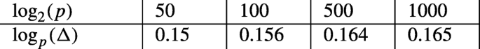
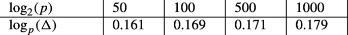
And it is certified that both heuristic and deterministic methods confirm the obtained bounds. We show the numerical results of the heuristic algorithms, which, on the other hand, also include the deterministic ones. We summarize its results in the following tables. We have selected primes of several sizes, and note the obtained success threshold.

• Theorem 2: Δ −approximations to k consecutive values and G public.

  • $k=2, {\Delta }=O(p^{1/6}), \frac {1}{6}= 0.16666$. Lattice dimension: 5.

    

  • $k=3, {\Delta }=O(p^{1/5}), \frac {1}{5}= 0.2$. Lattice dimension: 8

    

  • $k= 13, {\Delta }=O(p^{6/25}), \frac {6}{25}= 0.24$. Lattice dimension: 38

    

• Theorem 4: Δ −approximation to G and to k consecutive values.

  • $k=3, {\Delta }=O(p^{2/11}), \frac {2}{11}= 0.1818$. Lattice dimension: 9

    

  • $k= 13, {\Delta }=O(p^{12/61}), \frac {12}{61}= 0.1967$. Lattice dimension: 49

    

We have implemented the attack in SageMath-8.1 on a MacBook Pro laptop computer (3,3 GHz Intel Core i7, 16 GB RAM 2133 MHz LPDDR3 Mac OSX 10.12.6). Since the lattice dimension is very low -the biggest one is 49 which correspond the case k = 13 in Theorem 4- the time consuming in any trail is, as maximum, a couple of seconds.

6 Remarks and open questions

We have presented efficient algorithms for predicting the sequence produced by the linear congruential generator on elliptic curves. In fact, they only require computing a closest vector for a lattice of very low dimension, and for practical purposes can be used Babai’s Nearest Plane algorithm, see [2].

Following the ideas in [9] by generating more non-linear equations by multiplication of several non-linear equations before the linearization step, papers [31] and [32] present theoretical better bound O(p^1/5) for Theorem 1 and $O(p^{\frac {3k}{11k+4}})$ for Theorem 2, under the heuristic assumption that the created polynomials define a zero dimensional ideal. Their algorithm need to compute the LLL algorithm of a certain lattice of huge dimension and, after that, it also requires a Groebner Basis computation or alternatively any other elimination polynomial method. In practice the performance of the so called of Coppersmith’s methods in those cases are very bad because of large dimension of the lattice as it is shown in that papers. In fact, they can not test the bound $O(p^{\frac {3k}{11k+4}})$ not only because the large dimension but the size of the prime p should be several hundreds of bits. On the other hand, for instance, we can recover the sequence produced by EC-LCG if only three consecutive Δ −approximations are given as soon as Δ < p^1/5 requiring, the most time consuming, to compute a closest vector for a lattice of dimension 7 and it it matched by primes p of only 1000 bits.

As papers [31] and [32] show the bound of the size of the set of exceptional values of u₀ given in Theorem 1 is not tight and might be improved by more careful examination of the structure of (4) and (5) and this applies to Theorem 2.

Obviously the result in Theorem 3 is nontrivial only for Δ = O(p^1/6), we believe that this can be improvement to Δ = O(p^2/11) as Theorem 4 shows.

Giving rigorous proofs of our heuristic Theorem 2 and Theorem 4 is a challenging open question as well.

Same question has been studied in [32] for the Power Generator on elliptic curves: for a positive integer e > 1 and a point $G \in E(\mathbb {F}_{p})$ of order l with $\gcd (e,l)=1$, the elliptic curve Power Generator, (see [29]) generate a sequence of points V_n defined by the relation

$$V_{n} =[e^{n}]G$$

Requiring the prime p, integer e, constants a and b of the elliptic curve (1), and Δ −approximations W₀,W₁ to two consecutive values V₀,V₁ for ${\Delta } < p^{\frac {1}{2e^{2}}}$. An improvement is presented in [14] recovering the root U₀ = (x₀,y₀) of the polynomial (1) from a Δ −approximation to (x₀,y₀) as soon as Δ < p^1/7, considering the information given as approximation to the seed, in such a way that it is not taking advantage from the knowledge of the procedure which has generated them, see also [16]. We also think that better bounds are expected.

Another open problem is to mount an attack when the modulo p is unknown. Unfortunately, we do not know how to predict the EC-LCG when the modulus p is secret.

Finally, it would be interesting to study the security other PRBG based on elliptic curves under these type of attacks. In particular, it is not clear how to mount an attack based on the lattices to the Naor-Reingold Generator on Elliptic curves, see [36, 41, 42].

References

Avanzi, R., Cohen, H., Doche, C., Frey, G., Lange, T., Nguyen, K.K.: Elliptic and hyperelliptic curve crytography: Theory and practice. CRC Press (2005)
Babai, L.: On lovasz lattice reduction and the nearest lattice point problem. Combinatorica 6, 1–6 (1986)
Beelen, P., Doumen, J.: Pseudorandom Sequences from Elliptic Curves. Finite Fields with Applications to Coding Theory Cryptography and Related Areas, pp 37–52. Springer, Berlin (2002)
Blackburn, S., Gomez-Perez, D., Gutierrez, J., Shparlinski, I.: Predicting nonlinear pseudorandom number generators. Math. Comput. 74, 1471–1494 (2005)
Blake, I., Seroussi, G., Smart, N.: Elliptic curves in cryptography. London Math. Soc., Lecture Note Series, vol. 265. Cambridge Univ Press (1999)
Bloemer, J., May, A.: A tool kit for Finding small roots of Bivariate Polynomial over the Integers. Advances in Cryptology-Crypt. LNCS 2729, pp. 27–43. Springer (2003)
Boyar, J.: Inferring sequences produced by pseudo-random number generators. J. ACM 36, 129–141 (1989)
Brickell, E., Odlyzko, A.M.: Cryptanalysis: A survey of recent results. Contemp. cryptology, pp. 501–540. IEEE Press, NY (1992)
Coppersmith, D.: Small solutions to polynomial equations and low exponent RSA vulnerabilities. J. Cryptol. 10(4), 233–260 (1997)
Coppersmith, D.: Finding a Small Root of a Bivariate Integer Equations; Factoring with High Bits Known’. In: Maurer, U. (ed.) Proc. EUROCRYPT-96, LNCS 1070,155–156. Springer, Berlin (1996)
Coron, J. S.: Finding small roots of Bivariate Integer Polynomial Equations Revisted. Proc. Advances in Cryptology- Eurocrypt’04, LNCS, 3027, pp. 492–505. Springer (2004)
El Mahassni, E., Shparlinski, I.: On the Uniformity of Distribution of Congruential Generators over Elliptic Curves. Proc. Intern. Conf. on Sequences and Their Applications, 257–264 Bergen 2001. Springer, London (2002)
Frieze, A., Håstad, J., Kannan, R., Lagarias J. C., Shamir, A.: Reconstructing truncated integer variables satisfying linear congruences. SIAM J. Comp. 17, 262–280 (1988)
Gutierrez, J.: Reconstructing Points of Superelliptic Curves over a Prime Finite Field, Preprint. University of Cantabria (2021)
Gomez-Perez, D., Gutierrez, J., ibeas, A.: Attacking the Pollard Generator. IEEE. Trans. Inf. Theory. 52(12), 5518–5523 (2006)
Gomez-Perez, D., Gutierrez, J.: Recovering zeros of polynomials modulo a prime’. Math. Comput. 83(290), 2953–2965 (2014)
Gong, G., Berson, T., Stinson, D.: Elliptic Curve Pseudorandom Sequence Generators. Lect. Notes in Comp. Sci., vol. 1758, pp. 34–49. Springer, Berlin (2000)
Gong, G., Lam, C.: Linear recursive sequences over elliptic curves. Proc. Intern. Conf. on Sequences and their Applications, Bergen 2001, pp. 182-196. Springer, London (2002)
Grötschel, M., Lovász, L., Schrijver, A.: Geometric Algorithms and Combinatorial Optimization. Springer, Berlin (1993)
Gutierrez, J., Ibeas, A.: Inferring sequences produced by a linear congruential generator on elliptic curves missing high-order bits. Des. Codes Cryptogr. 45(2), 199–212 (2007)
Hallgren, S.: Linear congruential generators over elliptic curves. Preprint CS-94-143, pp. 1–10. Dept. of Comp. Sci. Cornegie Mellon University (1994)
Hess, F., Shparlinski, I.: On the linear complexity and multidimensional distribution of congruential generators over elliptic curves. Des. Codes Cryptogr. 35, 111–117 (2005)
Joux, A., Stern, J.: Lattice reduction: a toolbox for the cryptanalyst. J. Cryptol. 11, 161–185 (1998)
Jochemz, E., May, A.: A Strategy for Finding Roots of Multivariate Polynomials with New Applications in Attacking RSA Variants Advances in Cryptology (Asiacrypt 2006), Lecture Notes in Computer Science. Springer (2006)
Kannan, R.: Minkowski’s convex body theorem and integer programming. Math. Oper. Res. 12, 415–440 (1987)
Knuth, D.: Deciphering a linear congruential encryption. IEEE Trans. Inf. Theory. 31, 49–52 (1985)
Krawczyk, H.: How to predict congruential generators. J. Algorithm. 13, 527–545 (1992)
Lagarias, J.: Pseudorandom number generators in cryptography and number theory, vol. 42, pp. 115–143. Proc. Symp. in Appl. Math. Amer. Math. Soc., Providence (1990)
Lange, T., Shparlinski, I.: Certain exponential sums and random walks on elliptic curves. Canad. J. Math. 57, 338–350 (2005)
Lenstra, A., Lenstra, H., Lovász, L.: Factoring polynomials with rational coefficients. Math. Annalen. 261, 515–534 (1982)
Mefenza, T.: Inferring sequences produced by a linear congruential generator on elliptic curves using coppersmith’s methods. COCOON 2016 LNCS, vol. 9797, pp .293–304 (2016)
Mefenza, T., Vergnaud, D.: Inferring sequences produced by a elliptic Curves generators y using Coppersmith’s methods. Theor. Comput. Sci. 280, 20–42 (2020)
Meidl, W., Winterhof, A.: Linear Complexity of sequences and multisequences. , pp. 324–334. Handbook of Finite Fields, CRC Press, Taylor and Francis, Group. edits G. Mullen and D. Panario (2013)
Mérai, L.: Remarks on pseudorandom binary sequences over elliptic curves. Fund. Inf. 114(3-4), 301–308 (2012)
Mérai, L.: Predicting the elliptic curve congruential generator. Applicable Algebra in Engineering. Commun. Comput. 28(3), 193–203 (2017)
Naor, M., Reingold, O.: Number theoretic constructions of efficient pseudo-random functions. Proc 38th IEEE Symp. on Found. of Comp. Sci., pp. 458–467. IEEE (1997)
Niederreiter, H.: Design and Analysis of Nonlinear Pseudorandom Number Generators. In: Schueller, G.I., Spanos, P. D. (eds.) Monte Carlo Simulation, pp 3–9. A. Balkema Publishers, Rotterdam (2001)
Shparlinski, I.: Cryptographic applications of analytic number theory. Birkhauser (2003)
Shparlinski, I.: Orders of points on elliptic curves. Affine Algebraic Geometry. Amer. Math. Soc., pp. 245–252 (2005)
Shparlinski, I.: Pseudorandom Points on Elliptic Curves over Finite Fields. Recent trends in Cryptography. Contemporary Mathematics, v.477, Amer.Math. Soc., pp. 121–141 (2009)
Shparlinski, I: On the Naor-Reingold pseudo-random function from elliptic curves. Appl. Algebra Engin. Commun. Comput. 11, 27–34 (2000)
Shparlinski, I., Silverman, J.: On the linear complexity of the Naor-Reingold pseudorandom function from elliptic curves. Des. Codes Cryptogr. 24, 279–289 (2001)
Silverman, J.: The Arithmetic of Elliptic Curves. Springer, Berlin (1995)
Sun, H., Zhu, X., Zheng, Q.: Predicting truncated multiple recursive generators with unknown parameters. Des. Codes Cryptogr., pp. 1–20 (2020)
Winterhof, A.: Recent results on recursive nonlinear pseudorandom number generators. (Invited Paper). SETA 2010: 113–124 (2010)
Acknowledgements
The author wishes to thank Arne Winterhof for reading and commenting on a draft version.
Funding
Open Access funding provided thanks to the CRUE-CSIC agreement with Springer Nature.
Author information
Authors and Affiliations
Corresponding author
Additional information
Publisher’s note
Springer Nature remains neutral with regard to jurisdictional claims in published maps and institutional affiliations.
Rights and permissions
Open Access This article is licensed under a Creative Commons Attribution 4.0 International License, which permits use, sharing, adaptation, distribution and reproduction in any medium or format, as long as you give appropriate credit to the original author(s) and the source, provide a link to the Creative Commons licence, and indicate if changes were made. The images or other third party material in this article are included in the article's Creative Commons licence, unless indicated otherwise in a credit line to the material. If material is not included in the article's Creative Commons licence and your intended use is not permitted by statutory regulation or exceeds the permitted use, you will need to obtain permission directly from the copyright holder. To view a copy of this licence, visit http://creativecommons.org/licenses/by/4.0/.
About this article
Cite this article
Gutierrez, J. Attacking the linear congruential generator on elliptic curves via lattice techniques. Cryptogr. Commun. 14, 505–525 (2022). https://doi.org/10.1007/s12095-021-00535-6
Received:
Accepted:
Published:
Issue Date:
DOI: https://doi.org/10.1007/s12095-021-00535-6