The Internal Logic and Finite Colimits

Abstract

We describe how finite colimits can be described using the internal lanuage, also known as the Mitchell-Benabou language, of a topos, provided the topos admits countably infinite colimits. This description is based on the set theoretic definitions of colimits and coequalisers, however the translation is not direct due to the differences between set theory and the internal language, these differences are described as internal versus external. Solutions to the hurdles which thus arise are given.

Appendix A. Topos theory and logic

What is a logical connective? One interpretation of connectives is offered by ZF set theory. The axiom of specification allows for the manipulation of sets via the manipulation of predicates. For instance, if $\varphi (a),\psi (a)$ are formulas with free variable a, then the set $\lbrace a\in A \mid \varphi (a) \wedge \psi (a)\rbrace$ is given by the intersection of the sets $\lbrace a \in A \mid \varphi (a)\rbrace \cap \lbrace a \in A \mid \psi (a)\rbrace$.

In fact, this turns out to be a special case of a more general theory. The category $\underline{{\text {Sets}}}$ is an elementary topos, and indeed any elementary topos $\mathcal {E}$ offers a perspective on connectives. We show in this Section how the logical structure of the connectives $\forall , \exists , \wedge , \vee , \Rightarrow$ is captured by the categorical structure of $\mathcal {E}$.

1.1 A.1. Quantifiers

Definition A.1.1

Let $f: A \longrightarrow B$ be a morphism in a topos $\mathcal {E}$. We consider two copies of f and construct the pushout.

We then define the image of f to be the Equaliser of $\iota _1,\iota _2$.

$$\begin{aligned} {\text {im}}f := {\text {Equal}}(\iota _1,\iota _2) \end{aligned}$$

(110)

Theorem A.1.2

Let $\mathcal {E}$ be a topos and $f:A \rightarrow B$ a morphism. Then the functor $f^{-1}: \text {Sub}(B) \rightarrow \text {Sub}(A)$ admits both a left and a right adjoint.

Proof

See Johnstone [4, §A 1.4.10].

Definition A.1.3

Let $f:A \rightarrow B$ be a morphism in a topos. Then the left adjoint to $f^{-1}$ will be denoted $\exists _f$, and the right adjoint by $\forall _f$.

The reason why this notation is used, is because in the topos Set, these adjoints are given by the following explicit maps

$$\begin{aligned} \begin{array}{c} \exists _f: \text {Sub}(A) \rightarrow \text {Sub}(B)\\ A' \mapsto \lbrace b \in B \mid \text { there exists }a \in A'\text { such that }f(a) = b\rbrace \end{array} \end{aligned}$$

and

$$\begin{aligned} \begin{array}{c} \forall _f: \text {Sub}(A) \rightarrow \text {Sub}(B)\\ A' \mapsto \lbrace b \in B \mid \text { for all }a \in A\text { if }f(a) = b\text { then }a \in A'\rbrace \end{array} \end{aligned}$$

Proof

See [5, §1 9.2].

In the general context of an arbitrary topos, the left adjoint is particularly easy to describe.

Lemma A.1.4

Let $f:A \longrightarrow B$ be a morphism and let $m: M \rightarrowtail A \in {\text {Sub}}(A)$ be a subobject of A.

$$\begin{aligned} \exists _f(m) \cong {\text {im}}(fm) \end{aligned}$$

(111)

Proof

We will define a functor ${\text {im}}(f\underline{\hspace{0.2 cm}}): {\text {Sub}}A \longrightarrow {\text {Sub}}B$ and prove that this functor is left adjoint to the functor $f^{-1}: {\text {Sub}}B \longrightarrow {\text {Sub}}A$, the result will then follow from essential uniqueness of adjoints.

We define the image of a subobject $m: M \rightarrowtail A$ under ${\text {im}}(f\underline{\hspace{0.2 cm}})$ to be the subobject ${\text {im}}(fm)$ of B. Now we define how this functor behaves on morphims.

Let $m: M \rightarrowtail A, n:N \rightarrowtail A$ be subobjects of A and let $\gamma : M \longrightarrow N$ be a morphism such that the $m = n\gamma$. Let $i_1,i_2$ denote the morphisms such that ${\text {im}}(fm) = {\text {Equal}}(i_1,i_2)$ and let $i_1',i_2'$ denote the morphisms such that ${\text {im}}(fn) = {\text {Equal}}(i_1',i_2')$. To define a morphism ${\text {im}}(fm) \longrightarrow {\text {im}}(fn)$ it suffices to define a morphism $\gamma : C \longrightarrow C'$ such that $\gamma i_1 = i_1'$ and $\gamma i_2 = i_2'$. For convenience, we draw the following Diagram, we have denoted by C the object in the pushout ${\text {PushOut}}(fm,fm)$ and $C'$ for that of ${\text {PushOut}}(fn,fn)$.

We consider the following Diagram of solid arrows.

Since ${\text {im}}(fm)$ is a pushout, the existence of ${\text {im}}(f\gamma )$ which renders the Diagram commutative follows from the fact that $fm = fn \gamma$, which follows from the assumption that $m = n \gamma$.

Now we need to show that ${\text {im}}(f\underline{\hspace{0.2 cm}})$ is left adjoint to $f^{-1}$. That is, given $m: M \rightarrowtail A \in {\text {Sub}}A, r: R \rightarrowtail B \in {\text {Sub}}B$ along with a morphism $\delta :m \longrightarrow f^{-1}(r)$, we need to show that there exists a morphism $\eta _m: m \longrightarrow f^{-1}{\text {im}}(fm)$, natural in m, and a unique morphism $\beta :{\text {im}}(fm) \longrightarrow r$ such that the following Diagram commutes.

We make a note that $R \cong {\text {im}}r$, as r is monic, so it suffices to show the above statement with every instance of r replaced by ${\text {im}}r$. We overload the notation r and use this to denote the morphism ${\text {im}}r \rightarrowtail B$ as well as the morphism $R \rightarrowtail B$.

We let $i_1,i_2: B \longrightarrow C$ denote the morphisms such that ${\text {im}}(fm) = {\text {Equal}}(i_1,i_2)$, let $i_1',i_2': B \longrightarrow C'$ denote the morphisms such that ${\text {im}}(r) = {\text {Equal}}(i_1',i_2')$. First we define $\eta _m: m \longrightarrow f^{-1}{\text {im}}(fm)$. The natural morphism $\eta _m: M \longrightarrow f^{-1}{\text {im}}(fm)$ is given by pulling back ${\text {im}}(fm)$ along f and using the fact that fm factors through ${\text {im}}(fm)$. Naturally follows easily from universality of the objects involved. Now we show the eixstence of the morphism $\beta : {\text {im}}(fm) \longrightarrow r$. Consider the following Diagram of solid arrows.

Now, by the universal property of the equaliser ${\text {im}}r$, to show the existence of an appropriate morphism ${\text {im}}(fm) \longrightarrow {\text {im}}r$ it suffices to define a morphism $\zeta : C \longrightarrow C'$, denoted by a dashed arrow in (115), rendering (115) commutative. The objects $C,C'$ are respectively objects of pushouts, and so in turn it suffices to prove that $i_1' f m = i_2' f m$. This follows immediately from the fact that $i_1' r \alpha \delta = i_2' r \alpha \delta$.

1.2 A.2. Heyting algebras

Definition A.2.1

A Heyting algebra is a set with a partial order, which as a category admits the following.

• Initial and terminal objects.

• Binary products, binary coproducts.

• All exponentials.

Many examples are given by the following Theorem.

Theorem A.2.2

Let $\mathcal {E}$ be a topos, and let E be any object of $\mathcal {E}$. Then the set $\text {Sub}(E)$, with partial order given by inclusion, is a Heyting algebra with the relevant structure given as follows.

• Terminal object given by $\text {id}_E: E \rightarrow E$.

• Initial object given by the monic $0 \rightarrowtail E$, where 0 is the initial object of the topos $\mathcal {E}$. Note; this morphism $0 \rightarrowtail E$ is necessarily monic as $\mathcal {E}$ is a topos (see [4, §A1.4.1]).

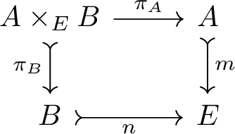
• The binary product of subobjects $m: A \rightarrowtail E$ and $n: B \rightarrowtail E$ is given by the triple $(A \times _{E} B,\pi _A,\pi _B)$, which is such that the following is a pullback diagram in $\mathcal {E}$.

  

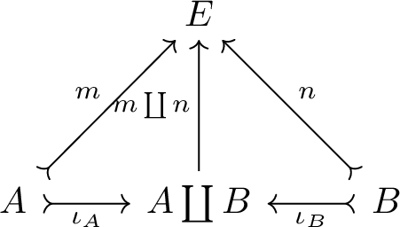
• The binary coproduct of subobjects $m: A \rightarrow E$ and $n: B \rightarrow E$ given by the triple ${({\text {Im}}(m\coprod n), k\iota _A,k\iota _B')}$ where ${(A \coprod B, \iota _A,\iota _B)}$ is a coproduct in $\mathcal {E}$, k is the induced morphism ${M \coprod N \longrightarrow {\text {im}}(m \coprod n)}$, and ${m \coprod n}$ is the unique morphism ${A \coprod B \rightarrow E}$ such that the following diagram commutes in $\mathcal {E}$.

  

• The exponentials are more complicated, see [4, §A1.4.13].

Proof

See [4, §A1.4].

Definition A.2.3

We denote the initial and terminal objects of a Heyting algebra by 0 and 1 respectively. The object corresponding to the binary product of objects A and B will be denoted $A \wedge B$, and the object corresponding the coproduct, $A \vee B$. Lastly, the objects $B^A$ will be denoted $A \Rightarrow B$.

Remark A.2.4

If $\mathcal {E}$ admits countably infinite coproducts, then for any object $E \in \mathcal {E}$, the Heyting algebra ${\text {Sub}}(E)$ also admits arbitrary coproducts. See [4, §A1.4]. If $\lbrace p_i \rbrace _{i \ge 0}$ is a countably infinite set of elements of ${\text {Sub}}(E)$ then the coproduct will be denoted by $\bigvee _{i\ge 0}p_i$.

1.3 A.3. Some helpful type theory lemmas

Many reasonable sounding statements concerning the entailment relation do in fact follow from the axioms and deduction rules, this section provides a collection of particularly helpful ones. Many of these will be used in Section 5. In what follows, $\Delta ,x:\tau$ will always mean the context given by appending $x:\tau$ to the end of the sequence $\Delta$, we give full proofs to illustrate the basic methods involved in working with type theories.

Lemma A.3.1

Let p, q, r be arbtirary formulas and $x:\tau$ an arbitrary variable.

• 1. $p \wedge q \vdash _\Delta r$ if and only if $q \wedge p \vdash _\Delta r$

• 2. $p \vdash _\Delta \lnot (\lnot p)$,

• 3. if $p \vdash _\Delta q$, then $p \wedge r \vdash _\Delta q$,

• 4. $\lnot q \vdash _\Delta \lnot (q \wedge p)$,

• 5. $p \wedge (q \vee r) \vdash _\Delta (p \wedge q) \vee (p \wedge r)$,

• 6. $(p \vee q) \wedge \lnot q \vdash _\Delta p$, and

• 7. $(\exists x:\tau , p) \wedge q \vdash _{\Delta }\exists x:\tau , p \wedge q$ and $\exists x:\tau , p \wedge q \vdash _{\Delta } (\exists x:\tau , p) \wedge q$

Proof

• 1. There is the following proof tree.

  

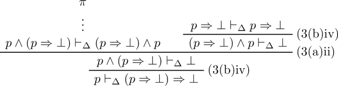
• 2. Let $\pi$ denote the following proof tree.

  

  Then, there is the following proof tree.

  

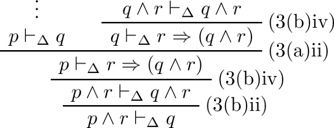
• 3. Observe the following proof tree.

  

• 4. By axiom $\mathrm{(3(b)iv)}$, it suffices to show $(q \Rightarrow \bot ) \wedge (q \wedge p) \vdash _\Delta \bot$, for which it suffices to show $((q \Rightarrow \bot ) \wedge q) \wedge p) \vdash _\Delta \bot$. By part 2 of this Lemma, it suffices to show $(q \Rightarrow \bot ) \wedge q \vdash \bot$, which follows from axiom $\mathrm{(3(b)iv)}$, as $q \Rightarrow \bot \vdash _\Delta q \Rightarrow \bot$.

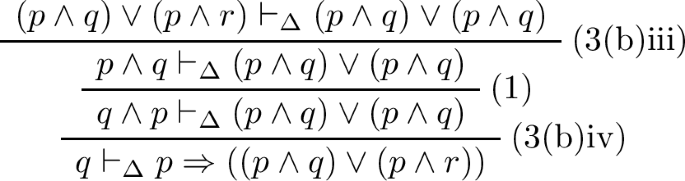
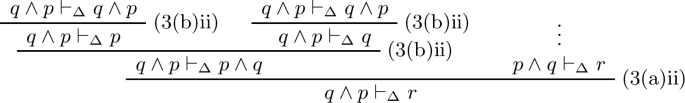
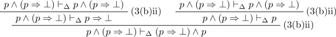
• 5. By $\mathrm{(3(b)iv)}$, it suffices to show $q \vee r \vdash _\Delta p \Rightarrow ((p \wedge q) \vee (p \wedge r))$, for which by (3(b)iii), it suffices to show both $q \vdash _\Delta p \Rightarrow ((p \wedge q) \vee (p \wedge r))$, and $r \vdash _\Delta p \Rightarrow ((p \wedge q) \vee (p \wedge r))$. The first sequent can be proved by the following, where the label (1) is referring to the first part of this Lemma.

  

  There is a similar proof tree for the remaining sequent.

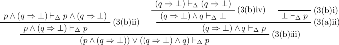
• 6. From part 4 of this Lemma, it suffices to show $(p \wedge \lnot q) \vee (\lnot q \wedge q) \vdash _\Delta p$, for which there is the following proof tree.

  

• 7. Observe the following proof tree.

  

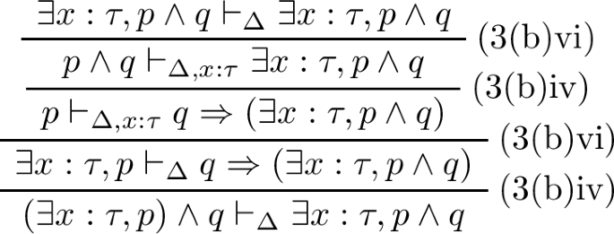
Reading this same proof tree from bottom to top gives a proof tree for the second sequent.

Lemma A.3.2

If $x:\tau$ is a variable, and $t:\tau$ is a term, then

$$\begin{aligned} x = t \vdash _{\Delta ,x:\tau }s \qquad \text {if and only if}\qquad \vdash _{\Delta }s[x := t] \end{aligned}$$

Proof

The “only if" direction follows from the following proof tree.

For the other direction, let $x':\tau$ be such that $x' \not \in \text {FV}(s)$, then there is the following proof tree.

Lemma A.3.3

If $p \vdash _{\Delta , x:\tau } q$, then $\exists x : \tau ,p \vdash _\Delta \exists x : \tau , q$.

Proof

First, let $\pi$ denote the following proof tree.

Then there is the following.

Lemma A.3.4

Let $t:\tau$ be a term and p a formula. Then

$$\begin{aligned} p[x := t] \vdash _{\Delta } \exists x : \tau , p \end{aligned}$$

The term t can be thought of as a witness of the statement p, so this Lemma states that to entail $\exists x : \tau , p$, it suffices to bear a witness t.

Proof

Observe the following proof tree,

Lemma A.3.5

If $p \vdash q$ then $p \vdash q \vee r$.

Proof

Observe the following proof tree.

References

Russell, B., Whitehead, A.: The Principles of Mathematics. Cambridge University Press, Cambridge (1903)
Lambek, J., Scott, P.J.: Introduction to Higher Order Categorical Logic. Cambridge University Press, New York (1986)
Sorensen, M., Urzyczyn, P.: Lectures on the Curry-Howard Isomorphism. Elsevier Science, Amsterdam (2006)
Johnstone, P.: Sketches of an Elephant. Clarendon Press, Oxford, A Topos Theory Compendium (2002)
Meordijk, I., Mac Lane, S.: Sheaves in Geometry and Logic. Springer, New York (1992)
Mikkelson, C. J.: Lattice Theoretic and Logical Aspects of Elementary Topoi. Aarhus Universitet, Matematisk Institut (1976)
May, J.: A Crash Course in Algebraic Topology. University of Chicago Press, Chicago (1999)
Borceux, F.: Handbook of Categorical Algebra 1. Basic Category Theory. University Press, Cambridge (1994)
Godel, K.: Uber formal unentscheidbare Sätze der Principia Mathematica und verwandter Systeme I. Monatshefte für Mathematik und Physik 38, 173–198 (1931)
Turing, A.: On computable numbers, with an application to the Entscheidungs problem. In: Proceedings of the London Mathematical Society (1936)
Church, A.: A Note on the Entscheidungsproblem. The Association for Symbolic Logic Inc, New York (1936)
Lawvere, W.: An elementary theory of the category of sets. Proc. Natl. Acad. Sci. USA 52, 1506–1511 (1964)
MacLane, S.: Homology. Springer, Berlin (1969)
Troiani, W.: Simplicial sets are algorithms. Masters Thesis. http://therisingsea.org/notes/MScThesisWillTroiani.pdf
Paré, R.: Colimits in Topoi. Bull. Am. Math. Soc. (1974)
Author information
Authors and Affiliations
Corresponding author
Additional information
Publisher's Note
Springer Nature remains neutral with regard to jurisdictional claims in published maps and institutional affiliations.