Distribution for Non Symmetric Position Operators on the Free Toy Fock Space and Its Approximation on the Full Fock Space

Abstract

In this paper, we investigate the “Poisson-type” limit theorem with respect to the vacuum state of a family of partial sums of non-symmetric position operators under an appropriate scaling on the free toy Fock space. We give a formula for the vacuum moment in relation with the combinatorics of non-crossing partitions. We show that the asymptotic measure associated to the limit of the partial sums of these operators is the free Meixner law with an atomic and an absolutely continuous part, whereas the probability distribution of any single operator is the two-point probability. The approximation of such operators on the full Fock space is given.

1 Introduction

Free probability is a branch of noncommutative probability theory. It was started by Voiculescu in the 80’s [18,19,20] in order to deal with some problems on operator algebras and calculating distributions of noncommutative random variables. A noncommutative probability space is a couple $(\mathcal {A}, \varphi )$ of a (unital) $*$-algebra $\mathcal {A}$ and a state $\varphi$ on it. The state $\varphi$ plays the role of the expectation in classical probability. The self-adjoint elements $a=a^*\in \mathcal {A}$ are called noncommutative random variables.

The notion of independence in free probability is called free independence (or freeness) which is analogous to the classical (or tensor) independence in classical probability. It was introduced by Voiculescu [18] and it allows to compute the mixed moments using the marginal distributions as for tensor independence in classical probability. Recall that a family of unital sub-algebras $\{\mathcal {A}_i, i\in {{\mathbb {N}}}\}$ with the same unit of $\mathcal {A}$ is called free independent if $\varphi (a_1\cdots a_n)=0$ for $a_j\in \mathcal {A}_{i(j)}$ whenever $\varphi (a_k)=0$ for all $k=1, \ldots , n$ and $i(1)\ne i(2)\ne \cdots \ne i(n-1)\ne i(n)$. Here, only the neighboring random variables do not belong to the same algebra, there is no assumption otherwise. Noncommutative random variables are called free independent if the subalgebras they generate are free independent. Many tools in classical probability have been established in the free setting. For instance, one gets free central limit theorem, where the Gaussian distribution is replaced by the Wigner distribution, or the Poisson theorem, where the Poisson law is replaced by Marchenko-Pastur distribution.

The free (full) Fock space is a basic structure for free probability theory. It is described as a direct sum of n-folds tensor product of a given Hilbert space $\mathcal {H}$, i.e., $\bigoplus _{n\ge 0}\mathcal {H}^{\otimes n}$, where $\mathcal {H}^{\otimes 0}:=\mathbb {C}\Omega$, and $\Omega$ is a distinguished norm one vector, called the vacuum vector.

We recall that in classical probability, the Brownian motion can be realized on the symmetric Fock space with the tensor independence as the sum of creation and annihilation operators [6], where the Gaussian law appears to be the distribution of such operators. This realization can be made also in the free probability by considering the sum of free creation and free annihilation operators acting on the free Fock space with freeness and the distribution of such operators is the Wigner law.

The free toy Fock space was introduced by Attal and Nechita [2] as a discrete type of the full Fock space, based on a free product of Hilbert spaces. The free toy Fock space can be seen, from a probabilistic point of view, as the smallest noncommutative probability space supporting a free family of Bernoulli random variables. It is shown in [2] that the free toy Fock space can be embedded into the full Fock space. Moreover, with this embedding, some elementary operators on the free toy Fock space approach its continuous counterparts operators on the full Fock space.

Generally, the (noncommutative) Poisson limit theorem (known also as law of small numbers) can be formulated by considering limit of arrays of (noncommutative) independent random variables. It was established by Speicher [17] for free independence, Muraki [11] for monotone independence, Wysoczański and the present author [14] for bm-independence. Another way of formulating Poisson-type limit theorem related to the discrete Fock space and its basic operators, was firstly established by Muraki [10] for monotone independence, Crismale et al. [3] for weakly-monotone independence, and recently the present author and Wysoczański [13] for bm-independence. The construction considered is as follows:

For $i\in {{\mathbb {N}}}$, consider the sum $A_{i}^{+}+A_{i}^{-}+\lambda A_{i}^{\circ }$ of a creation operator $A_{i}^{+}$, annihilation operator $A_{i}^{-}$ and a scalar multiple $\lambda \ge 0$ (which called the intensity) of a preservation operator $A_{i}^{\circ }$ on an appropriate discrete model Fock space. For $N\in {{\mathbb {N}}}$, set

$$\begin{aligned} S_{N}(\lambda ):=\frac{1}{\sqrt{N}}\sum _{i=1}^{N}(A_{i}^{+}+A_{i}^{-})+\lambda \sum _{i=1}^{N}A_{i}^{\circ }. \end{aligned}$$

(1)

Then, for every $p\in {{\mathbb {N}}}$, the limits

$$\begin{aligned} m_p(\lambda ):=\lim _{N\rightarrow +\infty } \varphi ((S_N(\lambda ))^p) \end{aligned}$$

describe a moments sequence of a distribution $\nu _\lambda$, called the “Poisson-type measure”. Here, $\varphi (\cdot ):=\langle \cdot \Omega , \Omega \rangle$ is the vacuum state, where $\Omega$ is the so-called vacuum vector. For weakly-monotone case [3], the associated measure belongs to the free Meixner law. For monotone independence, the probability measure has been identified by Muraki [10], whereas for bm-independence [13], the measure is still unknown. However, its moments $m_p(\lambda )$ are related to all noncrossing partitions consisting of pair or singleton blocks with bm-order.

In this paper, we extend this framework to the free toy Fock space, considered as a discrete type of the full Fock space. It turns out that in this case, the Poisson-type measure $\nu _\lambda$ of the operators $S_{N}(\lambda )$ belongs to the free Meixner class as for the single operator $S_{1}(\lambda ):=A_{i}^{+}+A_{i}^{-}+\lambda A_{i}^{\circ }$ in the case of weakly-monotone independence [3], whereas the measure $\nu _{1,\lambda }$ associated to the single operator $S_{1}(\lambda )$ in our case is the Bernoulli distribution as for monotone case [10].

The paper is structured as follows. In Sect. 2, we recall some basic knowledge about the noncommutative probability and the free toy Fock space with related creation, annihilation and conservation operators on it. We also recall some elementary information about noncrossing partitions of a finite set. Section 3 contains our main results: we perform analogous of the free Poisson-type limit theorem on the free toy Fock space. We start with the single case $S_{1}(\lambda )$, and show that the measure is the Bernoulli distribution, whereas the general case $S_{N}(\lambda )$ has the free Meixner distribution. In addition, we describe the moments sequence of the operators $S_{N}(\lambda )$ in relation with the combinatorics of noncrossing partitions. Finally, using the embedding of the free toy Fock space into the full Fock space, we investigate an approximation of the operators $S_{N}(\lambda )$ on the free toy Fock space with a continuous-time operators in the full Fock space.

2 Preliminaries

In this section we present some basic knowledge and definitions for our study.

2.1 Basic Notions of Noncommutative Probability

In what follows, $(\mathcal {A}, \varphi )$ stands for a noncommutative probability space, that is, a unital $*$-algebra $\mathcal {A}$ and a linear functional $\varphi : \mathcal {A}\rightarrow {{\mathbb {C}}}$, called state, such that $\varphi (a^*a)\ge 0$ for all $a\in \mathcal {A}$ and $\varphi (1_{\mathcal {A}})=1$ for the unit element $1_{\mathcal {A}}\in \mathcal {A}$. The state $\varphi$ plays a similar role as the expectation in classical probability. A noncommutative random variable is a self-adjoint element $a=a^{*}\in \mathcal {A}$, and its distribution (with respect to $\varphi$) is given by the probability measure $\nu _a$ such that

$$\begin{aligned} \varphi (a^n)=\int _{-\infty }^{+\infty }t^n\nu _a(dt), \end{aligned}$$

where $(\varphi (a^n))_{n\ge 0}$ denotes the moment sequence, when the moment problem is answered.

For more details in the framework of noncommutative probability, we refer the readers to [5, 7, 15] and references therein.

2.2 Partitions of a Finite Set

For a positive integer p, we denote by $[p]:=\{1, \ldots , p\}$. The collection $\pi :=\{B_1, \ldots , B_k\}$ of disjoint non-empty subsets $B_i$ of [p] whose union is [p] is called a partition with blocks $B_1, \ldots , B_k$, i.e.,

$$\begin{aligned} B_i\cap B_j=\emptyset \text{ for } i\ne j \text { and } \cup _{j=1}^{k}B_j=[p]. \end{aligned}$$

A block $B_i\in \pi$ is called singleton if $|B_i|=1$, where |.| denotes the cardinality, and it is called pair block if $|B_i|=2$. The set of all partitions $\pi$ of [p] is denoted by $\mathcal {P}(p)$. The number of blocks in $\pi$ is denoted by $|\pi |$ and the numbers of singletons by $s(\pi )$.

We say that a partition $\pi :=\{B_1, \ldots , B_k\}$ has a crossing if there exists at least two different blocks $B_i$ and $B_j$, and elements $a, b\in B_i, c, d\in B_j$ for which $a<c<b<d$. Otherwise, we say that $\pi$ is noncrossing and we denote the set of all noncrossing partitions of [p] by $\mathcal{N}\mathcal{C}(p)$ (sometimes we use $\mathcal{N}\mathcal{C}(p, k)$ to indicate number of blocks k).

For a partition $\pi =\{B_1, \ldots , B_k\}\in \mathcal {P}(p)$, there is a natural partial order $\preceq _\pi$ defined on the blocks of $\pi$ as follows:

$$\begin{aligned} B_i\preceq _{\pi } B_j \text { if } \min B_i\le \min B_j\le \max B_j\le \max B_i \end{aligned}$$

or

$$\begin{aligned} B_i\prec _{\pi } B_j \text { if } \min B_i< \min B_j\le \max B_j<\max B_i \end{aligned}$$

where $\min$ (resp. $\max$) is the minimum (resp. maximum) element of the block B.

For a partition $\pi$ with k blocks $B_1, \ldots , B_k$, we will use the notation $\pi :=(B_1, B_2, \ldots , B_k)$ to indicate that $\min B_j<\min B_{j+1}$ for $1\le j\le k-1$. In particular, we have $1\in B_1$.

A block $B_i\in \pi \in \mathcal{N}\mathcal{C}(p)$ is called inner if there exists another block $B_j$ such that $B_j\prec _{\pi }B_i$. Otherwise, it is called outer.

A noncrossing partition $\pi =\{B_1, \ldots , B_k\}\in \mathcal{N}\mathcal{C}(p, k)$ with $|B_j|\in \{1, 2\}$ for $j=1, \ldots , k$ is called noncrossing partition consisting of singletons or pair blocks, and the set of such a partitions is denoted by $\mathcal{N}\mathcal{C}_{1}^{2}(p)$ or $\mathcal{N}\mathcal{C}_{1}^{2}(p, k)$. On the other hand, it is called pair partition if $|B_j|=2$, for all $j=1, \ldots , k$, and we will use the notation $\mathcal{N}\mathcal{C}_{2}(p)$ for the set of all such a partitions.

The following two subsets of $\mathcal{N}\mathcal{C}_{1}^{2}(p)$ contribute in our study in the subsequent section.

• (1) The subset $\mathcal{N}\mathcal{C}_{1, i}^{2, o}(p)\subset \mathcal{N}\mathcal{C}_{1}^{2}(p)$ in which the partitions have no inner pair blocks and no outer singletons.

• (2) The subset $\mathcal{N}\mathcal{C}_{1, i}^{2}(p)\subset \mathcal{N}\mathcal{C}_{1}^{2}(p)$ of all partitions consisting of inner singletons (pair block can be either inner or outer).

For a partition $\pi \in \mathcal{N}\mathcal{C}_{1}^{2}(p)$, we denote by ${\tilde{\pi }}$ the reduced partition after removing the singletons of $\pi$, that is,

$$\begin{aligned} {\tilde{\pi }}:=\pi \setminus \{\text { singletons }\}\in \mathcal{N}\mathcal{C}_{2}(p-s(\pi )). \end{aligned}$$

In particular, for $\pi \in \mathcal{N}\mathcal{C}_{2}(p)$, we have $\pi ={\tilde{\pi }}$.

Graphically, for $p\in {{\mathbb {N}}}$, we present a partition $\pi =(B_1, \ldots , B_k)\in \mathcal {P}(p)$ by putting all numbers from the set [p] (in increasing order) on a horizontal line from the right to the left, and joint all numbers which belong to the same block by lines above. In particular, singletons are presented by vertical lines. For instance, consider the partition $\pi =(B_1, B_2, B_3, B_4)\in \mathcal {P}(8)$, where $B_{1}=\{1\}, B_{2}=\{2, 4\}, B_{3}=\{3, 5\}$ and $B_4=\{6, 7, 8\}$. Then the partition $\pi$ can be presented graphically as follows:

Definition 2.1

Let $\mathcal {I}$ be an arbitrary set of indices and $\pi =\{B_1, \ldots , B_k\}$ be a partition of [p]. A label function with values in $\mathcal {I}$ is a map $\textrm{L}: \pi \rightarrow \mathcal {I}$ such that $\textrm{L}(B_j)\in \mathcal {I}$ for $1\le j\le k$.

Definition 2.2

For two blocks $B_i\preceq _{\pi }B_j$, we say that a block $B_j$ is a direct successor of a block $B_i$ (equivalently, $B_i$ is a direct predecessor of $B_j$) if there is no any other block $B_l$ such that

$$\begin{aligned} B_i\preceq _{\pi }B_l\preceq _{\pi }B_j. \end{aligned}$$

Let $(i_p, \ldots , i_1)\in {{\mathbb {N}}}^p$ be a sequence of elements, and denote by k the cardinality of the set $\{i_p, \ldots , i_1\}$. For $j\in \{i_p, \ldots , i_1\}$, we define $B(j):=\{1\le m\le p: i_m=j\}\subset [p]$, and for $m\ne n$, we have either $B(i_m)=B(i_n)$ or $B(i_m)\cap B(i_n)=\emptyset$. Then, we obtain a partition $\pi =(B_1, \ldots , B_k)\in \mathcal {P}(p)$ of [p], such that for each $1\le l\le k$, we have $B_l=B(i_m)$ for some $1\le m\le p$. In this case, we say that the partition $\pi$ is adapted to the sequence $(i_p, \ldots , i_1)$ and we will use the notation $(i_p, \ldots , i_1)\sim \pi$ or $\pi \sim (i_p, \ldots , i_1)$. Moreover, for $j\in \{i_p, \ldots , i_1\}$, $\textrm{L}(B(j))$ will be called the label of the block B(j) and $(\textrm{L}(B_k), \ldots , \textrm{L}(B_1))$ will be called the label sequence of the partition $\pi$.

Remark 2.3

For $(i_p, \ldots , i_1)\sim \pi =\{B_1, \ldots , B_k\}$, the sets $\{i_p, \ldots , i_1\}$ and $\{\textrm{L}(B_1), \ldots , \textrm{L}(B_k)\}$ are identified.

Definition 2.4

Let $\pi =\{B_{1}, \ldots , B_{k}\}\in \mathcal{N}\mathcal{C}^{2}_{1}(p)$ and $(i_p, \ldots , i_1)\in [1, N]^p$ such that $(i_p, \ldots , i_1)\backsim \pi$. We say that the sequence $(i_p, \ldots , i_1)$ establishes free-labelling on the partition $\pi$ (notation $(i_p, \ldots , i_1)\blacktriangleright \pi$) if for all $1\le l\ne m\le k$ the following conditions hold:

• (1) If $|B_m|=2, B_{l}\preceq _{\pi }B_{m}$ and $B_m$ is a direct successor of $B_l$, then $\textrm{L}(B_l)\ne \textrm{L}(B_m)$

• (2) If $|B_m|=1, B_{l}\preceq _{\pi }B_{m}$ and $B_m$ is a direct successor of $B_{l}$, then $\textrm{L}(B_{l})=\textrm{L}(B_m)$

In this case, we say that the label sequence $(\textrm{L}(B_k), \ldots , \textrm{L}(B_1))$ establishes free-labelling on $\pi$ and we will use the notation $(\textrm{L}(B_k), \ldots , \textrm{L}(B_1))\blacklozenge \pi$.

Definition 2.5

Let N be a positive integer. For $\pi \in \mathcal{N}\mathcal{C}^{2}_{1}(p, k)$, we define the following sets:

$$\begin{aligned} \textrm{FL}(\pi , N):= & {} \{(i_p, \ldots , i_i)\in [1, N]^p: (i_p, \ldots , i_i)\sim \pi \quad \text { and }\quad (i_p, \ldots , i_i)\blacktriangleright \pi \}\\ \mathcal{F}\mathcal{L}(\pi , N):= & {} \{(\textrm{L}(B_k), \ldots , \textrm{L}(B_1)): \textrm{L}(B_j)\in [1, N], 1\\ {}\le & {} j\le k \text { and } (\textrm{L}(B_k), \ldots , \textrm{L}(B_1))\blacklozenge \pi \}. \end{aligned}$$

Using the information above, one obtains the following result about the cardinality of the set $\mathcal{F}\mathcal{L}(\pi , N)$ for a non crossing pair partition $\pi$.

Proposition 2.6

For a noncrossing pair partition $\pi$, one has

(2)

where the notation $\pi =\pi _{1}\cup \pi _{2}\cup \cdots \cup \pi _{k}$ is understood as a disjoint union of k subpartitions with exactly one outer block. Moreover,

$$\begin{aligned} \lim _{N\rightarrow +\infty }\frac{|\mathcal{F}\mathcal{L}(\pi , N)|}{N^{|\pi |}}=1. \end{aligned}$$

(3)

2.3 Free Toy Fock Space

The free toy Fock space was constructed by Attal and Nechita in [2]. In this section, we briefly recall this construction and some related aspects.

Let $\mathcal {H}$ be a separable complex Hilbert space with a fixed orthonormal basis $(e_i)_{i\ge 1}$, and define the full Fock space as

$$\begin{aligned} \mathcal {F}(\mathcal {H})=\bigoplus _{n=0}^{\infty }\mathcal {H}^{\otimes n}, \end{aligned}$$

where $\mathcal {H}^{\otimes 0}:=\mathbb {C}\Omega$ is a one -dimensional Hilbert space and $\Omega$ is a distinguished vector with norm one, which is called the vacuum vector.

The free creation and annihilation operators with the “test function" $f\in \mathcal {H}$, denoted by $l^+(f)$ and $l^-(f)$, respectively, are defined as

$$\begin{aligned} l^+(f)\Omega =f, \quad l^+(f)e_1\otimes \cdots \otimes e_n=f\otimes e_1\otimes \cdots \otimes e_n \end{aligned}$$

and

$$\begin{aligned} l^-(f)\Omega =0, \quad l^-(f)e_1\otimes \cdots \otimes e_n=\langle f, e_1\rangle e_2\otimes \cdots \otimes e_n. \end{aligned}$$

For $T\in \mathcal {B}(\mathcal {H})$, we define the so-called gauge operator (or second quantization operator) $\Lambda (T)$, as follows

$$\begin{aligned} \Lambda (T)\Omega =0, \quad \Lambda (T)e_1\otimes \cdots \otimes e_n=T(e_1)\otimes e_2\otimes \cdots \otimes e_n. \end{aligned}$$

Since

$$\begin{aligned} \Vert l^+(f)\Vert =\Vert l^-(f)\Vert =\Vert f\Vert \quad \text {and}\quad \Vert \Lambda (T)\Vert =\Vert T\Vert , \end{aligned}$$

they can be extended by linearity and continuity to the whole space, where $l^+(f)$ and $l^{-}(f)$ are mutually adjoint.

In what follows, we will consider the case where $\mathcal {H}=L^2(\mathbb {R}_+, \mathbb {C})$ is the complex Hilbert space of square integrable complex valued functions. Hence, one can redefine the creation, annihilation and gauge operators in the free (full) Fock space $\mathcal {F}(L^2(\mathbb {R}_+, \mathbb {C}))$. Note that an element $f\in \mathcal {F}(L^2(\mathbb {R}_+, \mathbb {C}))$ admits a decomposition $f=f_0+\sum _{n\ge 1}f_n$, where $f_0\in \mathbb {C}$ and $f_n\in L^2(\mathbb {R}^n_+)$. For an arbitrary $h\in L^2(\mathbb {R}_+)$, we denote the creation (resp. annihilation) operator by $A^+(h)$ (resp. $A^-(h)$), and are defined as follows:

$$\begin{aligned} A^+(h)\Omega= & {} h, \quad A^+(h)f_n(x_1, \ldots , x_{n+1})=h(x_1)f_n(x_2, \ldots , x_{n+1})\\ A^-(h)\Omega= & {} 0, \quad A^-(h)f_n(x_2, \ldots , x_{n})= \int h(x_1)f_n(x_1, x_2, \ldots , x_{n})dx_1. \end{aligned}$$

Moreover, for an essentially bounded function $g\in L^{\infty }(\mathbb {R}_+)$, one can define the gauge operator $A^{\circ }(g)$ associated to the operator of multiplication by g as follows:

$$\begin{aligned} A^{\circ }(g)\Omega =0, \quad A^{\circ }(g)f_n(x_1, \ldots , x_{n})=g(x_1)f_n(x_1, \ldots , x_{n}). \end{aligned}$$

In particular, for $t\in \mathbb {R}_+$ and $\mathbb {1}_t:=\mathbb {1}_{[0, t)}$ denotes the indicator function of the interval [0, t), we set $A^{\varepsilon }_t:=A^{\varepsilon }(\mathbb {1}_t)$ for $\varepsilon \in \{+, -, \circ \}$.

Definition 2.7

For a positive integer n, we say that a given sequence $(i_n, \ldots , i_1)\in \mathbb {N}^n$ is admissible, if $i_1\ne i_2 \ldots \ne i_n$. We assume by convention that the empty set $\emptyset$ is admissible, and we denote by ${\textbf {I}}_n$ the set of all admissible sequences of size n, and by ${\textbf {I}}$ the set of all admissible sequences of finite size.

For $i\in \mathbb {N}$, let $\mathcal {H}_i=\mathbb {C}^2$ be a two-dimensional complex Hilbert spaces, and denote by $\bigstar$ the free product. The free toy Fock space in the sequel denoted by $\mathcal {T}\mathcal {F}(L^2(\mathbb {R}_+, \mathbb {C}))$ is a countable free product of two-dimensional complex Hilbert spaces $\mathcal {H}_i=\mathbb {C}^2$, and is given by

$$\begin{aligned} \mathcal {T}\mathcal {F}(L^2(\mathbb {R}_+, \mathbb {C}):=\bigstar _{i\in \mathbb {N}}({{\mathbb {C}}}^{2}_{(i)}, \Omega _i)=\mathbb {C}\Omega \oplus \bigoplus _{n\ge 1}\bigoplus _{i_1\ne i_2\ne \cdots \ne i_n}\mathbb {C}X_{i_1}\otimes \cdots \otimes X_{i_n}, \end{aligned}$$

where $\mathbb {C}^{2}_{(i)}$ is the i-th copy of $\mathbb {C}^2=\mathcal {H}_i$ which is endowed with the canonical basis $\{\Omega _i=(1, 0)^T, X_i=(0, 1)^T\}$ and $\Omega$ is the common identification of the vacuum vectors $\Omega _i$ with $\Vert \Omega \Vert =1$. The orthonormal basis of $\mathcal {T}\mathcal {F}(L^2(\mathbb {R}), \mathbb {C})$ is given by $\{X_{{\textbf {i}}}\}_{{\textbf {i}}\in {\textbf {I}}}$ where $X_{{\textbf {i}}}$ is the tensor $X_{i_1}\otimes \cdots \otimes X_{i_n}$ for ${\textbf {i}}=(i_1, \ldots , i_n)$ and $X_{\emptyset }=\Omega$.

2.3.1 The Embedding of the Free Toy Fock Space into the Full Fock Space

It is shown in [1, 2] that the free toy Fock space can be embedded into the full Fock space $\mathcal {F}(L^2(\mathbb {R}_+; \mathbb {C}))$. Let us briefly recall this embedding: Consider a partition $S=\{0=t_0<t_1<\cdots<t_n<\cdots \}$ of $\mathbb {R}_+$ with diameter $d(S):=\sup _i|t_{i+1}-t_{i}|$. The associated full Fock space with this decomposition is given as follows

$$\begin{aligned} \mathcal {F}(L^2(\mathbb {R}_+; \mathbb {C}))=\bigstar _{i\in \mathbb {N}}\mathcal {F}(L^2([t_i, t_{i+1})) \end{aligned}$$

and in each Fock space $\mathcal {F}(L^2[t_i, t_{i+1}))$, we consider the vacuum vector $\Omega _i$ such that $|\Omega _i|=1$, and the normalized function

$$\begin{aligned} X_i:=\frac{\mathbb {1}_{[t_i, t_{i+1})}}{\sqrt{t_{i+1}-t_i}}=\frac{\mathbb {1}_{t_{i+1}} -\mathbb {1}_{t_i}}{\sqrt{t_{i+1}-t_i}}, \end{aligned}$$

where $\mathbb {1}_{[t_i, t_{i+1})}$ denotes the indicator function of the interval $[t_i, t_{i+1})$.

The free toy Fock space $\mathcal{T}\mathcal{F}(S)$ associated to the partition S is a closed subspace of the full Fock space $\mathcal {F}(L^2(\mathbb {R}_+; \mathbb {C}))$, and is given by:

$$\begin{aligned} \mathcal{T}\mathcal{F}(S)=\bigstar _{i\in \mathbb {N}}(\mathbb {C}\Omega _i\oplus \mathbb {C}X_i). \end{aligned}$$

For $t\in \mathbb {R}_+$ and $\epsilon \in \{-, +, \circ \}$, the relation between the operators $A_{t}^{\epsilon }$ on the full Fock space $\mathcal {F}(L^2(\mathbb {R}_+; \mathbb {C}))$ and their discrete counterparts $A_{i}^{\epsilon }$ on the free toy Fock space $\mathcal{T}\mathcal{F}(S)$ is given as follows: For a partition $S=\{0=t_0<t_1<\cdots<t_n<\cdots \}$ of $\mathbb {R}_+$ and $\epsilon \in \{-, +, \circ \}$, the basic operators $A_{i}^{\epsilon }(S)$ associated to the partition S on the free toy Fock space $\mathcal{T}\mathcal{F}(S)$ are given by

$$\begin{aligned} A_{i}^{\pm }(S)= & {} P_S\frac{A_{t_{i+1}}^{\pm }-A_{t_i}^{\pm }}{\sqrt{t_{i+1}-t_i}}P_S =P_SA^{\pm }\Big (\frac{\mathbb {1}_{[t_i t_{i+1})}}{\sqrt{t_{i+1}-t_i}}\Big )P_S\\ A_{i}^{\circ }= & {} P_S(A_{t_{i+1}}^{\circ }-A_{t_i}^{\circ })P_S=P_SA^{\circ }\big (\mathbb {1}_{[t_i, t_{i+1})}\big )P_S \end{aligned}$$

where $P_S\in \mathcal {B}(\mathcal {F}(L^2(\mathbb {R}_+; \mathbb {C})))$ denotes the orthogonal projection on the free toy Fock space $\mathcal{T}\mathcal{F}(S)$.

Proposition 2.8

[2] The operators $A_{i}^{+}(S), A_{i}^{-}(S)$ and $A_{i}^{\circ }(S)$ act on the free toy Fock space $T\Phi (S)$ in the same way as their discrete counterparts $A_{i}^{+}, A_{i}^{-}$ and $A_{i}^{\circ }$, respectively.

In what follows, we consider a partition $S_{n}:=\{0=t_{0}^{(n)}<\cdots<t_{l}^{(n)}<\cdots \}$ with $d(S_{n})\rightarrow 0$ for n going to infinite, and we denote by $A_{i}^{\epsilon }(n):=A_{i}^{\epsilon }(S_n)$ for $\epsilon \in \{-, +, \circ \}$. Finally, we get $\mathcal{T}\mathcal{F}(n):=\mathcal{T}\mathcal{F}(S_n)$. The following result from [2] plays significant role in our study.

Theorem 2.9

[2] For all $t\in \mathbb {R}_+$, the following operators

$$\begin{aligned} A_{t}^{\pm }(n)&:=\sum _{i;t_i^{(n)}\le t}\sqrt{t_{i+1}^{(n)}-t_{i}^{(n)}} A_{i}^{\pm }(n)\\ A_{t}^{\circ }(n)&:=\sum _{i;t_i^{(n)}\le t} A_{i}^{\circ }(n) \end{aligned}$$

converge strongly (as $n\rightarrow +\infty$) to $A_{t}^{\pm }$ and $A_{t}^{\circ }$, respectively.

3 Main Results

For $n\ge 1$, let ${\textbf {i}}:=(i_n, \ldots , i_1)\in {{\textbf {I}}}$ be an arbitrary non-empty admissible sequence and let $\mathbb {1}$ denotes the indicator function. Consider the free toy Fock space $\mathcal {T}\mathcal {F}(L^2(\mathbb {R}_+, \mathbb {C}))$ with the orthonormal basis $\{X_{{\textbf {i}}}\}_{{\textbf {i}}\in {{\textbf {I}}}}$. We define the creation $A_{X_i}^{+}$, annihilation $A_{X_i}^{-}$ and conservation $A_{X_i}^{\circ }$ operators in $\mathcal {T}\mathcal {F}(L^2(\mathbb {R}_+, \mathbb {C}))$ with the “test function” $X_i$, as the image of $A^{+}, A^{-}$ and $A^{\circ }$, respectively, acting on ${{\mathbb {C}}}^{2}_{i}$, as follows:

• (1) The creation operator $A_{i}^{+}:=A_{X_i}^{+}$ $A_{i}^{+}\Omega =X_i$, $A_{i}^{+}(X_{i_p}\otimes \cdots \otimes X_{i_1})=\mathbb {1}_{i\ne i_p}X_{i}\otimes X_{i_p}\otimes \cdots \otimes X_{i_1}$.

• (2) The annihilation operator $A_{i}^{-}:=A_{X_i}^{-}$ $A_{i}^{-}\Omega =0$, $A_{i}^{-}(X_{i_p}\otimes \cdots \otimes X_{i_1})=\mathbb {1}_{i = i_p} X_{i_{p-1}}\otimes \cdots \otimes X_{i_1}$.

• (3) The conservation operator $A_{i}^{\circ }:=A_{X_i}^{\circ }$ $A_{i}^{\circ }\Omega =0$, $A_{i}^{\circ }(X_{i_p}\otimes \cdots \otimes X_{i_1})=\mathbb {1}_{i=i_p}X_{i_p}\otimes \cdots \otimes X_{i_1}$.

These operators are bounded, and $A_{i}^{+}$ and $A_{i}^{-}$ are mutually adjoint (i.e., $(A_{i}^{+})^*=A_{i}^{-}$). Moreover, the conservation operator $A_{i}^{\circ }$ is self-adjoint and satisfies

$$\begin{aligned} A_{i}^{\circ }=A_{i}^{+}A_{i}^{-}. \end{aligned}$$

(4)

Furthermore, the following relations hold

$$\begin{aligned} \begin{aligned}&A_{i}^{\circ }A_{i}^{-}=A_{i}^{+}A_{i}^{+}=A_{i}^{-}A_{i}^{-}=0,\\&A_{j}^{\circ }A_{i}^{\circ }=A_{j}^{-}A_{i}^{\circ }=A_{j}^{\circ }A_{i}^{+}=A_{j}^{-}A_{i}^{+}=0, \quad i\ne j \end{aligned} \end{aligned}$$

(5)

Using (5) one can prove the following lemma.

Lemma 3.1

For any positive integers i, j and m, one has

$$\begin{aligned} \begin{aligned} A_{i}^{-}A_{i}^{+}A_{j}^{+}&=\mathbb {1}_{i\ne j}A_{j}^{+},\\ (A_{i}^{\circ })^{m}A_{i}^{+}&=A_{i}^{+}. \end{aligned} \end{aligned}$$

(6)

Definition 3.2

For any integer $p\ge 2$, we denote by $E_p$ the set of all sequences $\varvec{\epsilon }=(\epsilon _p, \ldots , \epsilon _1)\in \{-1, 0,+1\}^p$ which satisfy the following conditions:

• (1) $\epsilon _{1}=+1, \epsilon _{p}=-1,$

• (2) $\sum \limits _{i=1}^{p}\epsilon _{i}=0,$

• (3) $\sum \limits _{i=1}^{k}\epsilon _{i}\ge 0$   for $k=1, \ldots , p-1.$

It is known that there is a bijection between the set $E_p$ defined above and the set $\mathcal{N}\mathcal{C}_{1}^{2}(p)$ of all noncrossing partitions consisting of pair or singleton blocks. Let us recall this bijection from [13] (see also [8]).

Given a sequence $\varvec{\epsilon }=(\epsilon _p, \ldots , \epsilon _1)\in E_p$, for any $1\le k<p$ for which $\epsilon _k=+1$, we define

$$\begin{aligned} M(k):=\min \bigg \{j: j>k \text { and } \sum _{i=k}^{j}\epsilon _i=0\bigg \}. \end{aligned}$$

(7)

It follows that $\epsilon _{M(k)}=-1$, and for all $k<l<M(k)$ such that $\epsilon _l=+1$, we have

$$\begin{aligned} M(l)<M(k). \end{aligned}$$

Therefore, for any sequence $\varvec{\epsilon }=(\epsilon _p, \ldots , \epsilon _1)$ we can uniquely associate a noncrossing partition consisting of pair or singleton blocks as follows:

$$\begin{aligned} \pi :=\big \{\{k, M(k)\}: \epsilon _k=+1\big \}\cup \big \{\{j\}: \epsilon _j=0\big \}\in \mathcal{N}\mathcal{C}_{1}^{2}(p). \end{aligned}$$

In such a case, we will use the identification $\varvec{\epsilon }\equiv \pi$, for $\varvec{\epsilon }\in E_p$ and $\pi \in \mathcal{N}\mathcal{C}_{1}^{2}(p)$.

The following two lemmas, can be proven by a simple induction on p, and using the same arguments as in [13].

Lemma 3.3

Let $(\epsilon _p, \ldots , \epsilon _1)\in \{-1, 0, +1\}^p$ and $(i_p, \ldots , i_1)\in [1, N]^p$. If $\varvec{\epsilon }\notin E_p$, then

$$\begin{aligned} \varphi (A_{i_p}^{\epsilon _p}\cdots A_{i_1}^{\epsilon _1})=0. \end{aligned}$$

Lemma 3.4

Let $\varvec{\epsilon }=(\epsilon _p, \ldots , \epsilon _1)\in \{-1, 0, +1\}^p$ and $(i_p, \ldots , i_1)\in [1, N]^p$. If $\varphi (A_{i_p}^{\epsilon _p}\cdots A_{i_1}^{\epsilon _1})\ne 0$, then for every $1\le k\le p-1$ such that $\epsilon _k=+1$, we have $i_{M(k)}=i_k$.

In the following result, we describe the relation between the sequence $(i_p, \ldots , i_1)\in [1, N]^p$ and the mixed-moments $\varphi (A_{\epsilon _p}^{i_p} \cdots A_{\epsilon _1}^{i_1})$.

Lemma 3.5

[free-labelling and vanishing of mixed-moments] Let $\pi =(B_1, \ldots , B_k)\in \mathcal{N}\mathcal{C}_{1}^{2}(p)$ be a noncrossing partition with blocks being pair or singletons, and let $\varvec{\epsilon }=(\epsilon _p, \ldots , \epsilon _1)\in E_p$. Let us take ${{\textbf {i}}}=(i_p, \ldots , i_1)\in [1, N]^p$ such that $\varvec{\epsilon }\equiv \pi$ and ${{\textbf {i}}}\sim \pi$. If $\varphi (A_{i_p}^{\epsilon _p}\cdots A_{i_1}^{\epsilon _1})\ne 0$, then ${{\textbf {i}}}\blacktriangleright \pi$.

Proof

We proceed the proof by induction on $p\ge 2$. Obviously, for $p=2$ and $p=3$, the sequences $(i_2, i_1)$ and $(i_3, i_2, i_1)$ establish free-labelling.

For general induction, let $\pi \in \mathcal{N}\mathcal{C}_{1}^{2}(p)$ and we consider the following cases:

• (1) $M(1)<p$. In this case, we have

  

  where $\pi '\in \mathcal{N}\mathcal{C}_{1}^{2}(M(1))$ and $\pi ''\in \mathcal{N}\mathcal{C}_{1}^{2}(p-M(1))$ are sub-partitions of $\pi$ such that $\pi '\equiv (i_{M(1)}, \ldots , i_1)$ and $\pi ''\equiv (i_p, \ldots , i_{M(1)+1})$. According to Lemma 3.4 and by the induction assumption, we obtain

  $$\begin{aligned} 0\ne A_{i_{M(1)}}^{-}\cdots A_{i_1}^{+}\Omega =\Omega . \end{aligned}$$

  (8)

  Then,

  $$\begin{aligned} \varphi (A_{i_{M(1)}}^{-}\cdots A_{i_1}^{+})=1\ne 0 \end{aligned}$$

  and

  $$\begin{aligned} \varphi (A_{i_p}^{-}\cdots A_{i_{M(1)+1}}^{+}A_{i_{M(1)}}^{-}\cdots A_{i_1}^{+})&=\langle A_{i_p}^{-}\cdots A_{i_{M(1)+1}}^{+}A_{i_{M(1)}}^{-}\cdots A_{i_1}^{+}\Omega , \Omega \rangle \\&=\langle A_{i_p}^{-}\cdots A_{i_{M(1)+1}}^{+}\Omega , \Omega \rangle \\&=\varphi (A_{i_p}^{-}\cdots A_{i_{M(1)+1}}^{+})\ne 0, \end{aligned}$$

  where in the second equality we use (8). Hence, the induction can be applied to the sequences

  $$\begin{aligned} (i_{M(1)}, \ldots , i_{1})\sim \pi ' \text { and } (i_{p}, \ldots , i_{M(1)+1})\sim \pi ''. \end{aligned}$$

• (2) The case $M(1)=p$. We claim that the partition has only one outer block $\{1, M(1)\}$ as follows:

  

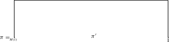
  where $\pi '\in \mathcal{N}\mathcal{C}_{1, i}^{2}(p-2)$. Indeed, we define $j:=\min \{l, 2\le l\le p, \epsilon _l=-1\}$, and we are looking at the first annihilation operator $A_{i_j}^{\epsilon _j}$. For $j=2$, we have one pair block $\{1, 2\}$ and $p=M(1)=2$. On the other hand, for $j=p$, the partition has only one outer block $\{1, p\}$ and $p-2$ singleton inner blocks. In any case, the sequence $(i_p, \ldots , i_1)$ establishes free-labelling on $\pi$. For $2< j <p$, we have $\epsilon _k\in \{+1, 0\}$ for $2\le k\le j-1$. Assume that there exists an index $2\le k\le j-1$ which satisfies $\epsilon _k=0$, and define

  $$\begin{aligned} k':=\min \{k: 2\le k\le j-1, \epsilon _k=0\}. \end{aligned}$$

  Therefore, $\epsilon _i=+1$ for all $1\le i\le k-1$. By induction assumption and by the commutation relation (5), one obtains

  $$\begin{aligned} i_{k'}=i_{k'-1}\ne \cdots \ne i_2\ne i_1 \end{aligned}$$

  and

  $$\begin{aligned} A_{i_j}^{-}\cdots A_{i_{k'}}^{\circ }A_{i_{k'-1}}^{+}A_{i_{k'-2}}^{+}\cdots A_{i_2}^{+}A _{i_1}^{+}\Omega =A_{i_j}^{-}\cdots A_{i_{k'+1}}^{\epsilon _{k'+1}}A_{i_{k'-1}}^{+}A_{i_{k'-2}}^{+} \cdots A_{i_2}^{+}A_{i_1}^{+}\Omega \ne 0 \end{aligned}$$

  Moreover,

  $$\begin{aligned} \varphi (A_{i_p}^{\epsilon _p}\cdots A_{i_1}^{\epsilon _1})=\varphi (A_{i_p}^{-}A_{i_{p-1}}^{\epsilon _{p-1}}\cdots A_{i_{j+1}}^{\epsilon _{j+1}}A_{i_j}^{-}A_{i_{j-1}}^{\epsilon _{j-1}}\cdots A_{i_{k'+1}}^{\epsilon _{k'+1}}A_{i_{k'-1}}^{+}A_{i_{k'-2}}^{+}\cdots A_{i_1}^{+})\ne 0 \end{aligned}$$

  and the sequence $(i_p, \ldots , i_{k'+1}, i_{k'-1}, \ldots , i_1)\in [1, N]^{p-1}$ establishes free-labelling on the partition $\pi '=\pi \setminus \{k'\}\in \mathcal{N}\mathcal{C}_{1}^{2}(p-1)$. Taking into account that the singleton block $\{k'\}$ is a direct successor of the pair block $\{k'-1, M(k'-1)\}$, and the pair blocks $\{n, M(n)\}$ are direct successors of the pair blocks $\{n-1, M(n-1)\}$ for $n=2, \ldots , k'-1$, respectively. Then,

  $$\begin{aligned} (i_p, \ldots , i_1)\blacktriangleright \pi \in \mathcal{N}\mathcal{C}_1^2(p). \end{aligned}$$

  Now, assume that $\epsilon _k=+1$ for all $1\le k\le j-1$. Then, $j=M(j-1)$, and by induction assumption

  $$\begin{aligned} i_j=i_{M(j-1)}\ne i_{M(j-1)-1}\ne \cdots \ne i_2\ne i_1. \end{aligned}$$

  According to Lemma 3.1, we have

  $$\begin{aligned} \varphi (A_{i_p}^{\epsilon _p}\cdots A_{i_1}^{\epsilon _1})=\varphi (A_{i_p}^{-}\cdots A_{i_{j+1}}^{\epsilon _{j+1}}A_{i_{j-2}}^{\epsilon _{j-2}}\cdots A_{i_1}^{+})\ne 0 \end{aligned}$$

  and

  $$\begin{aligned} (i_p, \ldots , i_{j+1}, i_{j-2}, \ldots i_1)\blacktriangleright \pi '\in \mathcal{N}\mathcal{C}_{1}^{2}(p-2). \end{aligned}$$

  Hence, the lemma follows, since $i_j=i_{j-1}\ne i_{j-2}\ne \cdots \ne i_1$, and the pair block $\{j-1, j\}$ is a direct successor of the block $\{j-2, M(j-2)\}$.

$\square$

Corollary 3.6

Let $(\epsilon _p, \ldots , \epsilon _1)\equiv \pi \in \mathcal{N}\mathcal{C}_{1}^{2}(p)$ and ${{\textbf {i}}}=(i_p, \ldots , i_1)\in [1, N]^p$ such that ${{\textbf {i}}}\sim \pi$. If $\varphi (A_{i_p}^{\epsilon _p}\cdots A_{\epsilon _1}^{i_1})\ne 0$, then all singleton blocks in $\pi$ must be inner, i.e., $\pi \in \mathcal{N}\mathcal{C}_{1, i}^{2}(p)$.

Moreover, by induction on p and by Lemma 3.1, it follows that

$$\begin{aligned} \varphi (A_{i_p}^{\epsilon _p}\cdots A_{i_1}^{\epsilon _1})=1 \text { for } {{\textbf {i}}}\blacktriangleright \pi . \end{aligned}$$

(9)

3.1 Poisson-Type Limit Theorem

In this section, we will study the vacuum distribution for the operators

$$\begin{aligned} S_{N}(\lambda ):=\sum _{i=1}^{N}\Big (\frac{A_{i}^{+}+A_{i}^{-}}{\sqrt{N}}+\lambda A_{i}^{\circ }\Big )=\sum _{i=1}^{N}\Big (\frac{G_{i}}{\sqrt{N}}+\lambda A_{i}^{\circ }\Big ),\quad \lambda \ge 0 \end{aligned}$$

(10)

on the free toy Fock space $\mathcal {T}\mathcal {F}(L^2(\mathbb {R}_+, \mathbb {C}))$, where $G_{i}:=A_{i}^{+}+A_{i}^{-}$ is the free Gaussian process.

For the case $\lambda =0$, we obtain

$$\begin{aligned} S_{N}(0):=\frac{1}{\sqrt{N}}\sum _{i=1}^{N}G_{i} \end{aligned}$$

(11)

the free central limit theorem [9, 12, 21], where the associated (even) moments are the Catalan numbers $C_p:=\frac{1}{p+1} {2p\atopwithdelims ()p}$, and the distribution limit is the Wigner measure [19] supported on $[-2, 2]$. Namely,

$$\begin{aligned} \varphi ((S_{N}(0))^{2p})=C_p=\frac{1}{2\pi }\int _{-2}^{2}x^{2p}\sqrt{4-x^2}dx. \end{aligned}$$

Let us first start with the single operators $S_{1}(\lambda )$, that is,

$$\begin{aligned} S_{1}(\lambda )=A_{i}^{+}+A_{i}^{-}+\lambda A_{i}^{\circ }. \end{aligned}$$

(12)

It is clear that the family $\{A_{i}^{+}+A_{i}^{-}+\lambda A_{i}^{\circ }\}_{i\in {{\mathbb {N}}}}$ is free independent in the free toy Fock space $\mathcal {T}\mathcal {F}(L^2(\mathbb {R}_+, \mathbb {C}))$.

We denote by $b_{p}(\lambda ):=\varphi ((S_{1}(\lambda ))^p)$ the p-th moment of the operators $S_{1}(\lambda )$. The following theorem can be proven in similar way as in [13] for bm-independence.

Theorem 3.7

For any non-negative integer p, the moment sequence $(b_p(\lambda ))_{p\ge 0}$ of the operators $S_{1}(\lambda )$ is

$$\begin{aligned} b_{p}(\lambda )=\sum _{\pi \in \mathcal{N}\mathcal{C}_{1, i}^{2, o}(p)}\lambda ^{s(\pi )}, \end{aligned}$$

(13)

where in the sum appear the set of noncrossing partitions consisting of pair outer blocks or inner singleton blocks, and $s(\pi )$ denotes the number of singletons in $\pi$.

Moreover, we have the following recursive formula

$$\begin{aligned} b_{0}(\lambda )=1, b_{1}(\lambda )=0, b_{p}(\lambda )=b_{p-2}(\lambda )+\lambda b_{p-1}(\lambda ), \text { for } p\ge 2. \end{aligned}$$

(14)

Remark 3.8

By taking $\lambda =1$ in (14), we obtain the Fibonacci sequence.

Theorem 3.9

The distribution law $\nu _{1, \lambda }$ of the operators $S_{1}(\lambda )$ under the vacuum state $\varphi$ is the two-point distribution:

$$\begin{aligned} \nu _{1, \lambda }=a^-\delta _{x^{+}}+a^+\delta _{x_{-}} \end{aligned}$$

(15)

where $x_{\pm }=\frac{\lambda }{2}\pm \frac{\sqrt{\lambda ^2+4}}{2}$ and $a^{\pm }=\frac{1}{2}\pm \frac{\lambda }{2\sqrt{\lambda ^2+4}}$.

Proof

By Theorem 3.7, the direct calculations of the moment generating function $f_{\lambda }(t):=\sum \nolimits _{p\ge 0}b_{p}(\lambda )t^p$, yields

$$\begin{aligned} f_{\lambda }(t)=\frac{1-\lambda t}{1-\lambda t-t^2}, \end{aligned}$$

(cf. [16]). Then, using the Cauchy transform [21] and the Stieltjes inversion formula, we obtain (15). $\square$

Now let us turn to the general case by considering the limit distribution of the operators

$$\begin{aligned} S_{N}(\lambda )=\frac{1}{\sqrt{N}}\sum _{i=1}^{N}A_{i}^{+}+A_{i}^{-}+\lambda \sum _{i=1}^{N}A_{i}^{\circ } \quad \text { at } N\rightarrow +\infty \end{aligned}$$

(16)

under the vacuum state $\varphi$. After denoting $m_{p}(\lambda ):=\lim \nolimits _{N\rightarrow +\infty }\varphi ((S_{N}(\lambda ))^p)$, we have the following.

Theorem 3.10

For any non-negative integer p, the moment sequence $(m_p(\lambda ))_{p\ge 0}$ is given by the following

$$\begin{aligned} m_{p}(\lambda )=\sum _{\pi \in \mathcal{N}\mathcal{C}_{1, i}^{2}(p)}\lambda ^{s(\pi )}=:\sum _{\pi \in \mathcal{N}\mathcal{C}_{1, i}^{2}(p)}V(\pi , \lambda ) \end{aligned}$$

(17)

where in the sum appear all noncrossing partitions consisting of pair or inner singleton blocks.

Corollary 3.11

The function $V(\pi , \lambda )$ for $\pi \in \mathcal{N}\mathcal{C}_{1, i}^{2}(p)$ is multiplicative and can be given recursively as follows:

(18)

Proof of Theorem 3.10

We have

$$\begin{aligned} \varphi ((S_{N}(\lambda ))^p)=\frac{1}{N^{\frac{p}{2}}}\sum _{\epsilon _{1}, \ldots , \epsilon _p\in \{-1, 0, +1\}^p}\quad \sum _{i_1, \ldots , i_p\in [1, N]^p}\varphi (A_{i_p}^{\epsilon _p}\cdots A_{i_1}^{\epsilon _1})\lambda _N^{\sum _{k=1}^{p}\delta _0(\epsilon _k)}\nonumber \\ \end{aligned}$$

(19)

where $\lambda _N=\sqrt{N}\lambda$ and $\delta _{0}(\epsilon _{k})=\left\{ \begin{array}{ll} 1 &{} \hbox {if } \epsilon _{k}=0, \\ 0 &{} \hbox {otherwise.} \end{array} \right.$

By virtue of Lemma 3.1 and the commutation relations (4) and (5), one can show that

$$\begin{aligned} \varphi (A_{i_p}^{\epsilon _p}\cdots A_{i_j}^{\epsilon _j}\cdots A_{i_1}^{\epsilon _1})=0 \end{aligned}$$

where $i_j\ne i_k$ for all $1\le k,j\le p$.

According to Lemmata 3.3 and 3.5, and using the notations ${{{\textbf {i}}}}:=(i_p, \ldots , i_1), {\varvec{\epsilon }}:=(\epsilon _p, \ldots , \epsilon _1)$ and $A_{\varvec{\epsilon }}^{i}:=A_{\epsilon _p}^{i_p}\ldots A_{\epsilon _1}^{i_1}$, one obtains

$$\begin{aligned} \varphi \big ((S_{N}(\lambda ))^p\big )&= \frac{1}{N^{\frac{p}{2}}}\sum _{\varvec{\epsilon }\in E_p}\quad \sum _{{{\textbf {i}}}\in [1, N]^p}\varphi (A_{{{\textbf {i}}}}^{\varvec{\epsilon }})\lambda _{N}^{\sum _{k=1}^{p}\delta _0(\epsilon _k)}\\&=\frac{1}{N^{\frac{p}{2}}}\sum _{E_p\ni \varvec{\epsilon }\equiv \pi \in \mathcal{N}\mathcal{C}_{1}^{2}(p)}\quad \sum _{[1, N]^p\ni {{\textbf {i}}}\blacktriangleright \pi }\varphi (A_{{{\textbf {i}}}}^{\varvec{\epsilon }})\lambda _{N}^{\sum _{k=1}^{p}\delta _0(\epsilon _k)}. \end{aligned}$$

Since ${{\textbf {i}}}\blacktriangleright \pi$, the label sequence ${\textbf {l}}=(\textrm{L}(B_k), \ldots , \textrm{L}(B_1))$ establishes free-labelling on the partition $\pi =(B_1, \ldots , B_k)\in \mathcal{N}\mathcal{C}_{1}^{2}(p)$. Moreover, $|\mathcal{F}\mathcal{L}(\pi , N)|=|\mathcal{F}\mathcal{L}({\tilde{\pi }}, N)|$ for $\pi \in \mathcal{N}\mathcal{C}_{1}^{2}(p)$. Then, by virtue of Corollary 3.6, we have

$$\begin{aligned} \varphi \big ((S_{N}(\lambda ))^p\big )&=\frac{1}{N^{\frac{p}{2}}}\sum _{\pi \in \mathcal{N}\mathcal{C}_{1, i}^{2}(p)}\quad \sum _{{{\textbf {i}}}\in \textrm{FL}(\pi , N)}\lambda _N^{s(\pi )}\\&=\frac{1}{N^{\frac{p}{2}}}\sum _{\pi \in \mathcal{N}\mathcal{C}_{1, i}^{2}(p)}\quad \sum _{{\textbf {l}}\in \mathcal{F}\mathcal{L}(\pi , N)}\lambda _N^{s(\pi )}\\&=\sum _{\pi \in \mathcal{N}\mathcal{C}_{1, i}^{2}(p)}\frac{|\mathcal{F}\mathcal{L}({\tilde{\pi }}, N)|}{N^{|{\tilde{\pi }}|}}\lambda ^{s(\pi )} \end{aligned}$$

Taking limit on both sides above, the thesis follows. $\square$

Theorem 3.12

For $\lambda >0$, the vacuum distribution of $S_{N}(\lambda )$ converges for $N\rightarrow +\infty$ to the free Meixner law $\nu _{\lambda }(dx)$ with parameters $(\lambda , 1, 1, 0)$. Namely

$$\begin{aligned} \nu _{\lambda }(dx) = \left. {\left\{ \begin{array}{ll} \frac{1}{2\pi }\frac{\sqrt{4-(x-\lambda )^2}}{\lambda x+1}\mathbb {1}_{[\lambda -2, \lambda +2]}(x)dx &{} \text { if } 0<\lambda < 1 \\ \frac{1}{2\pi }\frac{\sqrt{4-(x-1)^2}}{x+1}\mathbb {1}_{(-1, 3]}(x)dx &{} \text { if } \lambda =1\\ \frac{\lambda ^2-1}{\lambda ^2}\delta _{\frac{-1}{\lambda }}+\frac{1}{2\pi }\frac{\sqrt{4-(x-\lambda )^2}}{\lambda x+1}\mathbb {1}_{[\lambda -2, \lambda +2]}(x)dx &{} \text { if } \lambda >1. \end{array}\right. } \right. \end{aligned}$$

Proof

Let $\pi =\pi _1\cup \cdots \cup \pi _k\in \mathcal{N}\mathcal{C}_{1, i}^{2}(p)$ be a disjoint union of k sub-partitions with exactly one outer block, such that

where $\pi '_j$ is an arbitrarily partition consisting of pair or inner singleton blocks, which can be also empty. Then

$$\begin{aligned} m_p(\lambda )&=\sum _{\pi \in \mathcal{N}\mathcal{C}_{1, i}^{2}(p)}V(\pi , \lambda )\\&=\sum _{k=1}^{\lfloor \frac{p}{2}\rfloor }\quad \sum _{\begin{array}{c} p_1+\cdots +p_k=p\\ p_1\ge 2, \ldots , p_k\ge 2 \end{array}}\quad \sum _{\pi _1\in \mathcal{N}\mathcal{C}_{1, i}^{2}(p_1), \ldots , \pi _k\in \mathcal{N}\mathcal{C}_{1, i}^{2}(p_k)}V(\pi _1, \lambda )\cdots V(\pi _k, \lambda ). \end{aligned}$$

Here $\lfloor x \rfloor$ denotes the greatest integer less than or equal to x.

Hence, the associated moment generating function $g_\lambda (t):=\sum \nolimits _{p\ge 0}m_{p}(\lambda )t^p$ is given as follows

$$\begin{aligned} g_\lambda (t)&= m_{0}(\lambda )t^0+\sum _{p\ge 2}\Bigg \{\sum _{k=1}^{\lfloor \frac{p}{2}\rfloor }\sum _{\begin{array}{c} p_1+\cdots +p_k=p\\ p_1\ge 2, \ldots , p_k\ge 2 \end{array}}\sum _{\pi _1\in \mathcal{N}\mathcal{C}_{1, i}^{2}(p_1), \ldots , \pi _k\in \mathcal{N}\mathcal{C}_{1, i}^{2}(p_k)}V(\pi _1, \lambda )\cdots V(\pi _k, \lambda )\Bigg \}t^p\\&= 1+\sum _{p\ge 2}\Bigg \{\sum _{k=1}^{\lfloor \frac{p}{2}\rfloor }\sum _{\begin{array}{c} p_1+\cdots +p_k=p\\ p_1\ge 2, \ldots , p_k\ge 2 \end{array}}\Biggl (\sum _{\pi _1\in \mathcal{N}\mathcal{C}_{1, i}^{2}(p_1)}V(\pi _1, \lambda )t^{p_1}\Biggr )\cdots \Biggl (\sum _{\pi _k\in \mathcal{N}\mathcal{C}_{1, i}^{2}(p_k)}V(\pi _k, \lambda )t^{p_k}\Biggr )\Bigg \} \\&= 1+\sum _{k\ge 1}\Bigg (\sum _{p_1\ge 2}\bigg (\sum _{\pi \in \mathcal{N}\mathcal{C}_{1, i}^{2}(p_1)}V(\pi , \lambda )\bigg )t^{p_1}\Bigg )^{k} =\frac{1}{1-h_\lambda (t)} \end{aligned}$$

where

$$\begin{aligned} h_\lambda (t)&=\sum _{n\ge 2}\Big \{\sum _{\pi \in \mathcal{N}\mathcal{C}_{1, i}^{2}(n)}V(\pi , \lambda )\Big \}t^n\\&=\sum _{n\ge 2}\left\{ \sum _{k=0}^{\lfloor \frac{n-2}{2}\rfloor }\left( {\begin{array}{c}n-2\\ 2k\end{array}}\right) \lambda ^{n-2-2k}C_{k}\right\} t^n=t^2\sum _{m\ge 2}\left\{ \sum _{k=0}^{\lfloor \frac{m}{2}\rfloor }\left( {\begin{array}{c}m\\ 2k\end{array}}\right) \lambda ^{m-2k}C_k\right\} t^m\\&=t^2\sum _{k\ge 0}C_k\lambda ^{-2k}\sum _{m=2k}^{+\infty }\left( {\begin{array}{c}m\\ 2k\end{array}}\right) (\lambda t)^m=\frac{(1-\lambda t)-\sqrt{(1-\lambda t)^2-4t^2}}{2} \end{aligned}$$

Note that in the last equality, we used the formula from [4]

$$\begin{aligned} \sum _{n\ge 0}\left( {\begin{array}{c}n\\ m\end{array}}\right) t^n=\frac{t^m}{(1-t)^{m+1}}, \end{aligned}$$

and the moment generating function of the Wigner law

$$\begin{aligned} \sum _{n\ge 0}C_nt^n=\frac{1-\sqrt{1-4t}}{2t}, \end{aligned}$$

where $C_n$ denote the Catalan numbers.

Hence, the moment generating function $g_\lambda (t)$ is given by

$$\begin{aligned} g_{\lambda }(t)=\frac{2}{1+\lambda t+\sqrt{(1-\lambda t)^2-4t^2}}. \end{aligned}$$

(20)

Therefore, the desired result follows through the Cauchy transform of the moment generating function $g_\lambda (t)$ (cf. [16, 21]). $\square$

Remark 3.13

It is worthwhile to mention that for the weakly-monotone independence case [3], the single operator $S_{1}(\lambda )=A_{i}^{+}+A_{i}^{-}+\lambda A_{i}^{\circ }$ on the weakly-monotone Fock space, has also the vacuum law belonging to the free Meixner class as for the general case $S_{N}(\lambda )$.

3.2 Examples

For illustration, in Table 1, we listed the first moments ($m_{0}(\lambda ), \ldots , m_{6}(\lambda )$) of free Poisson distribution in comparison with monotone and some of bm-analogues.

Table 1 The first moments $m_0(\lambda ), \ldots , m_{6}(\lambda )$ of free Poisson distribution, monotone Poisson distribution and bm-Poisson distribution for the cones ${{\mathbb {R}}}^2_+$ and ${{\mathbb {R}}}^3_+$

For $\lambda \ge 0$ and $n\ge 1$, we define the operators

$$\begin{aligned} Y_{i}^{(n)}(\lambda ):=A_{i}^{+}(n)+A_{i}^{-}(n)+\lambda \sqrt{n}A_{i}^{\circ }(n) \end{aligned}$$

(21)

on the free toy Fock space $\mathcal{T}\mathcal{F}(n)$. On the other hand, we define the operators

$$\begin{aligned} Y_{t}(\lambda ):=A_{t}^{+}+A_{t}^{-}+\lambda A_{t}^{\circ } \text { for } t\in \mathbb {R}_+, \end{aligned}$$

(22)

on the full Fock space $\mathcal {F}(L^2({{\mathbb {R}}}_+); {{\mathbb {C}}})$. For simplicity, we consider the sequence $S_n:=\{\frac{k}{n}, k\in {{\mathbb {N}}}\}$ for which $d(S_n)=\frac{1}{n}\rightarrow 0$. Then, we have the following approximations.

Theorem 3.14

Let $\lambda \ge 0, t\in {{\mathbb {R}}}_+$ and $n\ge 1$. Then,

• (1) The operators $Y_{i}^{(n)}(\lambda )$ are free independent and have the Bernoulli distribution

  $$\begin{aligned} \mu _{n, \lambda }=\alpha ^-\delta _{y^{+}}+\alpha ^+\delta _{y^{-}}, \end{aligned}$$

  (23)

  where $y_{\pm }=\frac{\sqrt{n}\lambda }{2}\pm \frac{\sqrt{n\lambda ^2+4}}{2}$ and $\alpha ^{\pm }=\frac{1}{2}\pm \frac{\sqrt{n}\lambda }{2\sqrt{n\lambda ^2+4}}$.

• (2) The operators

  $$\begin{aligned} Y_{t}^{(n)}(\lambda ):=\frac{1}{\sqrt{n}}\sum _{i=0}^{\lfloor nt\rfloor }Y_{i}^{(n)}(\lambda ) \end{aligned}$$

  converge (in the strong operator topology) as $n\rightarrow +\infty$ to the operators $Y_{t}(\lambda )$.

Proof

The proof of (23) follows from Proposition 2.8 and Theorem 3.9, by replacing $\lambda$ with $\sqrt{n}\lambda$.

For the proof of the second part, we have

$$\begin{aligned} Y_{t}^{(n)}(\lambda )&=\frac{1}{\sqrt{n}}\sum _{i=0}^{\lfloor nt \rfloor }Y_{i}^{(n)}(\lambda )\\&=\sum _{i; t_i^{(n)}\le t}\Big (\frac{1}{\sqrt{n}}A_{i}^{+}(n)+\frac{1}{\sqrt{n}}A_{i}^{-}(n)+\lambda A_{i}^{\circ }(n)\Big )\\&=\sum _{i; t_i^{(n)}\le t}\sqrt{t^{(n)}_{i+1}-t_{i}^{(n)}}\Big (A_{i}^{+}(n)+A_{i}^{-}(n)\Big )+\lambda \sum _{i; t^{(n)}\le t}A_{i}^{\circ }(n)\\&=A_{t}^{+}(n)+A_{t}^{-}(n)+\lambda A_{t}^{\circ }(n). \end{aligned}$$

Hence, the proof follows as an application of Theorem 2.9.

Corollary 3.15

For all integer $p\ge 2$, we have

$$\begin{aligned} \varphi ((Y_{i}^{(n)}(\lambda ))^p)=\sum _{\pi \in \mathcal{N}\mathcal{C}_{1, i}^{2, o}(p)}(\sqrt{n}\lambda )^{s(\pi )}. \end{aligned}$$

Moreover, for $\lambda =0$, the operator $Y_{t}^{(n)}(0)$ converges (in the strong operator topology), as $n\rightarrow +\infty$, to the distribution of a free Brownian motion $\{Y_t(0)\}_{t\in {{\mathbb {R}}}_+}$ (see Proposition 4, [2]).

References

Attal, S.: Approximating the Fock Space with the Toy Fock Space. Séminaire de probabilités, XXXVI. Lecture Notes in Mathematics, vol. 1801, pp. 477–491. Springer, Berlin (2003)
Attal, A., Nechita, I.: Discrete approximation of the free Fock space. In: Donati-Martin, C., Lejay, A., Rouault, A. (eds.) Séminaire de Probabilités XLIII. Lecture Notes in Mathematics, vol. 2006, pp. 379–394. Springer, Berlin, Heidelberg (2006/2011)
Crismale, V., Griseta, M.E., Wysoczański, J.: Distributions for nonsymmetric monotone and weakly monotone position operators. Complex Anal. Oper. Theory 15, 101 (2021). https://doi.org/10.1007/s11785-021-01146-y
Graham, R.L., DKnuth, D.E., Patashnik, O.: Concrete Mathematics. Addison-Wesley, New York (1989)
Hora, A., Obata, N.: Quantum Probability and Spectral Analysis of Graphs. Theoretical and Mathematical Physics. Springer, Berlin (2007)
Hudson, R.L., Parthasarathy, K.R.: Quantum Ito’s formula and stochastic evolutions. Commun. Math. Phys. 93(3), 301–323 (1984)
Meyer, P.A.: Quantum Probability for Probabilists. Lecture Notes in Mathematics, vol. 1538. Springer, Berlin (1993)
Młotkowski, W.: Limit theorems in \(\Lambda \)-boolean probability. Infinite Dimens. Anal. Quantum Probab. Relat. Top. 7(3), 449–459 (2004)
Muraki, N.: A new example of noncommutative “de Moivre-Laplace theorem”. In: Watanabe, S., Fukushima, M., Prohorov, Yu. V., Shiryaev, A.N. (eds.) Probability Theory and Mathematical Statistics. Proceeding of the Seventh Japan–Russia Symposium, Tokyo 1995, pp. 353–362. World Scientific, Singapore (1996)
Muraki, N.: Analogue of Poisson distribution in monotone Fock space, preprint (1999)
Muraki, N.: Monotonic independence, monotonic central limit theorem and monotonic law of small numbers. Infinite Dimens. Anal. Quantum Probab. Relat. Top. 4(1), 39–58 (2002)
Nica, A., Speicher, R.: Lectures on the Combinatorics of Free Probability. Cambridge University Press, Cambridge (2006)
Oussi, L., Wysoczański, J.: Analogues of Poisson-type limit theorems in discrete bm-Fock spaces. Infinite Dimens. Anal. Quantum Probab. Relat. Top. (2023). https://doi.org/10.1142/S0219025723500170
Oussi, L., Wysoczański, J.: Noncommutative analogue of the law of small numbers for random variables indexed by elements of positive symmetric cones. ALEA Lat. Am. J. Probab. Math. Stat. 18, 35–67 (2021)
Parthasarathy, K.R.: An Introduction to Quantum Stochastic Calculus. Birkhaüser, Basel (1992)
Saitoh, N., Yoshida, H.: The infinite divisibility and orthogonal polynomials with a constant recursion formula in free probability theory. Probab. Math. Stat. 21, 159–170 (2001)
Speicher, R.: A new example of “independence’’ and “white noise’’. Probab. Theory Relat. Fields 84(2), 141–159 (1990)
Voiculescu, D.V.: Symmetries of some reduced free product C\(*\)-algebras. In: Operator Algebras and their Connections with Topology and Ergodic Theory. Lecture Notes in Mathematics, vol. 1132. Springer, pp. 556–588 (1985)
Voiculescu, D.V.: Addition of certain noncommutative random variables. J. Funct. Anal. 66, 323–346 (1986)
Voiculescu, D.V.: Multiplication of certain non-commuting random variables. J. Oper. Theory 18(2), 223–253 (1987)
Voiculescu, D.V., Dykema, K.J., Nica, A.: Free Random Variables. CRM Monograph Series. AMS, Providence (1992)
Acknowledgements
The author sincerely appreciates the anonymous referee for his/her valuable comments and suggestions.
Author information
Authors and Affiliations
Contributions
The author reviewed the manuscript.
Corresponding author
Ethics declarations
Conflict of interest
The author has no conflict of interest to declare.
Additional information
Communicated by Christian Le Merdy.
Publisher's Note
Springer Nature remains neutral with regard to jurisdictional claims in published maps and institutional affiliations.
Rights and permissions
Open Access This article is licensed under a Creative Commons Attribution 4.0 International License, which permits use, sharing, adaptation, distribution and reproduction in any medium or format, as long as you give appropriate credit to the original author(s) and the source, provide a link to the Creative Commons licence, and indicate if changes were made. The images or other third party material in this article are included in the article’s Creative Commons licence, unless indicated otherwise in a credit line to the material. If material is not included in the article’s Creative Commons licence and your intended use is not permitted by statutory regulation or exceeds the permitted use, you will need to obtain permission directly from the copyright holder. To view a copy of this licence, visit http://creativecommons.org/licenses/by/4.0/.
About this article
Cite this article
Oussi, L. Distribution for Non Symmetric Position Operators on the Free Toy Fock Space and Its Approximation on the Full Fock Space. Complex Anal. Oper. Theory 17, 117 (2023). https://doi.org/10.1007/s11785-023-01422-z
Received:
Accepted:
Published:
DOI: https://doi.org/10.1007/s11785-023-01422-z
Keywords
- Noncommutative probability
- Free independence
- Free Fock space