
Abstract
Whether markets are efficient or not has been broadly discussed in the empirical literature since the efficient markets hypothesis was proposed by Fama and others in the 1960s. Unfortunately, they did not come to a consistent conclusion. Besides, while these studies show whether a specific market is efficient or not, little has been done to explore the issues regarding the degree of market inefficiency. This paper attempts to resolve the puzzle of the inconsistent conclusions in the empirical literature by adopting a bottom-up approach which takes market participants’ interactions and coordination into consideration. By simulating an agent-based artificial stock market, this paper concludes with three main findings. First, agents’ survivability is mainly decided by risk preference, and not forecasting accuracy. Survivors may have diverse forecasting accuracy. Second, because market prices are not decided by agents based on accurate predictions, markets can not be efficient. What may exist is only the difference of the degree of inefficiency between markets. Third, the more relevant to survivability the forecasting accuracy in a market is, the less inefficient the market will be. Therefore, this paper suggests that it may be better to view the divergent empirical results regarding market efficiency as a fact that markets are inefficient to a variety of degrees.


Notes
Forecasting accuracy only matters when agents share the same risk preferences in their market.
Log-utility traders are with a constant relative risk aversion (CRRA) coefficient of one.
The range of the RRA coefficient is based on existing intensive empirical studies.
By stepping away from this danger zone, they found that the relevance of the level of saving rates to the survivability of traders came to be revealed.
Stepping away from the danger zone means avoiding choosing the extremely low down-side saving rates.
The choice and definition of the likelihood is specified in the first paragraph of “Belief updating scheme” section of Appendix 1.
Fig. 2 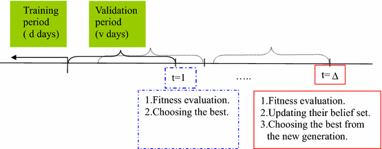
Belief updating scheme
This has been confirmed by the K-S statistic. See footnote 15 in Chen and Huang (2008).
All agents in Chen and Huang (2007) have the same length of validation period which is pertinent to forecasting accuracy.
If the market is efficient, \(p_{m,t} \) follows a random walk. Prices have a unit-root. That is, \(\ln (p_{m,t} )=\ln (p_{m,t-1} )+\varepsilon _t \) and \(\varepsilon _t \) should be an uncorrelated series (that is, an \(i.i.d.\) series). The return of asset \(m\) at time\(~t\), \(R_{m,t} \), is defined as \(R_{m,t} =\ln (p_{m,t} )-\ln (p_{m,t-1} )\) here. Therefore, in this section econometric tests are applied to the return series for \(i.i.d.\) to examine the efficiency of markets.
\(\sigma \): standard deviation. The tests on various parameters of the BDS test are shown in “Appendix 3”.
\(\tau _1 \) and \(\tau _2 \) are exogenous parameters. \(\tau _1 +\tau _2 \) is the number of bits for beliefs.

References
Ayadi OF, Pyum CS (1994) The application of the variance ratio test to the Korean securities market. J Bank Finance 18:643–658
Beveridge S, Oickle C (1997) Long memory in the Canadian stock market. Appl Financ Econ 7:667–672
Chaudhuri K, Wu Y (2003) Random walk versus breaking trend in stock prices: evidence from emerging markets. J Bank Finance 27:575–592
Chelly-Steeley P (2001) Mean reversion in the horizon returns of UK portfolios. J Bus Finance Account 28:107–126
Blume L, Easley D (1992) Evolution and market behavior. J Econ Theory 58:9–40
Blume L, Easley D (2006) If you’re so smart, why aren’t you rich? Belief selection in complete and incomplete markets. Econometrica 74(4):929–966
Brock WA, Dechert WD, LeBaron B, Scheinkman J (1996) A test for independence based on the correlation dimension. Econom Rev 15:197–235
Bullard J, Duffy J (1999) Using genetic algorithms to model the evolution of heterogeneous beliefs. Comput Econ 13(1):41–60
Chen S-H, Huang Y-C (2005) On the role of risk preference in survivability. In: Wang L, Chen K, Ong YS (eds) Advances in natural computation, lecture notes in computer science, vol 3612. Springer, pp 612–621
Chen S-H, Huang Y-C (2007) Relative risk aversion and wealth dynamics. Inf Sci 177(5):1222–1229
Chen S-H, Huang Y-C (2008) Risk preference, forecasting accuracy and survival dynamics: simulations based on a multi-asset agent-based artificial stock market. J Econ Behav Organ 67(3):702–717
Eldridge MR, Bernhardt C, Mulvey I (1993) Evidence of chaos in the S&P 500 cash index. Adv Futures Options Res 6:179–192
Fama EF, French KR (1988) Common factors in the serial correlation of stock returns. Center for Research in Security Prices Working Paper, no. 200
Greene MT, Fieltz BD (1977) Long term dependence in common stock returns. J Financ Econ 4:339–349
Hsieh DA (1991) Chaos and nonlinear dynamics: application to financial markets. J Finance 46:1839–1877
Kohers T, Pandey V, Kohers G (1997) Using nonlinear dynamics to test for market efficiency among the major US stock exchanges. Q Rev Econ Finance 37:523–545
Lee J, Strazicich MC (2003) Minimum LM unit root test with two structural breaks. Rev Econ Stat 85:1082–1089
Lee C-C, Lee J-D, Lee C-C (2009) Stock prices and the efficient market hypothesis: evidence from a panel stationary test with structural breaks. Japan and the World Economy. Corrected proof, available online 5 May 2009 (in press)
Lo AW, Mackinlay AC (1988) Stock market prices do not follow random walks: evidence from a simple specification test. Rev Financ Stud 1:41–66
Lo AW, Mackinlay AC (1989) The STZE and power of the Variance Ratio test in finite samples: a Monte Carlo investigation. J Econom 40:203–238
Narayan PK (2005) Are the Australian and New Zealand stock prices nonlinear with a unit root? Appl Econ 37:2161–2166
Narayan PK (2006) The behaviour of US stock prices: evidence from a threshold autoregressive model. Math Comput Simul 71:103–108
Narayan PK, Smyth R (2007) Mean reversion versus random walk in G7 stock prices evidence from multiple trend break unit root tests. J Int Financ Mark Inst Money 17:152–166
Opong KK, Sprevak D (2000) The behaviour of the Irish ISEQ index: some new empirical tests. Appl Financ Econ 10:693–700
Peter EE (1994) Fractal market analysis: applying chaos theory to investment and economics. Wiley, New York
Poterba JM, Summers LH (1988) Mean reversion in stock prices: evidence and implications. J Financ Econ 22:27–59
Qian XY, Song FT, Zhou WX (2008) Nonlinear behaviour of the Chinese SSEC index with a unit root: evidence from threshold unit root tests. Phys A Stat Mech Appl 387:503–510
Sandroni A (2000) Do markets favor agents able to make accurate predictions? Econometrica 68:1303–1341
Sciubba E (2006) The evolution of portfolio rules and the capital asset pricing model. J Econ Theory 29(1):123–150
Sewell SP, Stansell SR, Lee I, Pan MS (1993) Nonlinearities in emerging foreign capital markets. J Bus Finance Account 20:237–248
Acknowledgments
The author gratefully acknowledges the very helpful suggestions of several anonymous referees and the support provided by the National Science Council in the form of Grant no. NSC-97-2410-H-262-001.
Author information
Authors and Affiliations
Corresponding author
Appendices
Appendix 1
This appendix is mainly based on Chen and Huang (2008)’s supplementary data.
1.1 Evolution of beliefs
The investor revises and renews his investment strategies with respect to a specific belief selected from a population of beliefs \(\{ {B_{j,t}^i } \}_{j=1}^J\). In other words, at each point in time, the investor has more than one model of uncertainty in the world. Of course, these models are not equally promising, and the investor tends to base his decision (investment strategies) on one of the most promising ones. However, as time goes on, his beliefs of the world will be revised and renewed in light of the newly incoming information. In this section, we shall describe how the GA can be applied to modeling the beliefs updating process.
1.1.1 Coding and initialization
In the Blume–Easley–Sandroni model, each investor’s perception of the uncertainty (finite-state stochastic process) of the market can be characterized by two elements: first, the dependence structure \((k)\), and, second, the sample size \((d)\). Based on this characterization, the investor believes that the market over the last \(d\) days follows a \(k\hbox {th}\)-order Markov process. According to this belief, he would use a part of the historical data \(\left\{ {m_{t-s} } \right\} _{s=v+1}^{v+d+1},\) referred as to thetraining period, to estimate the Markov transition matrix, and the rest of the data \(\left\{ {m_{t-s} } \right\} _{s=1}^v \) referred to as the validation period, to validate the estimated model. As a result, each belief can be represented by a binary string, of length \(\tau 1 + \tau 2\),Footnote 11
that has the following interpretation: the states follow a Markov process of the order
over the last
days. To facilitate estimation, \(d\) cannot be too small, and that demands an additional constant \(c\). In our current model, we simplify and limit the dependent structure \((k)\) to 0 or 1, that is, the stochastic process is only assumed to be \(i.i.d.\) or first-order Markov.
At the initial date \((t = 0)\), all investors are endowed with a population of \(J\) beliefs, which are randomly generated. Then every \(\Delta \) days, this population of beliefs will be reviewed and revised based on the fitness function, which is a kind of likelihood function to be specified below.
1.1.2 Belief updating scheme
Agents follow the practice of machine learning. They are supposed to care about the risk of over-fitting, and hence use data in the validation period to perform model selection. One way of ensuring that agents behave so is to set the fitness function as the fitting error in the validation set, rather than the training set. Then a fitness measure for a beliefs \(B_{j,t}^i \) is its associated likelihood, evaluated by the validation set \(\left\{ {m_{t-s} } \right\} _{s=1}^v \)
Equation (18) is the likelihood of the observations \(\left\{ {m_{t-s} } \right\} _{s=1}^v \) in the validation period under the belief \(B_{j,t}^i \). Every \(\Delta \) periods, after they finish the evaluation of each belief’s fitness, they apply the genetic operation to update their belief set (see “Genetic operation” section of Appendix 1), and the belief with the highest fitness will be chosen. Even in the period in which the genetic operation is not applied, say, when \(t\in [\Delta +1,\, 2\Delta -1]\), they evaluate the fitness of beliefs in their current belief set using the newest data and choose the best from it.
1.1.3 Genetic operation
Once the procedure of evaluating each belief’s fitness is completed, all beliefs are associated with a fitness which is the output of (18).
Based on this fitness evaluation, investor \(i\)’s beliefs are revised and renewed by using four genetic operators: selection, crossover, mutation and election.
1.1.4 Loops
After a new belief is generated by these operators, a loop in Fig. 7 will lead investor \(i\) back to selection, which is then followed by crossover, mutation and election before the next belief is generated. The loop will continue until all \(J\) beliefs of \(\{ {B_{j,t}^i } \}_{j=1}^J\) are generated. One of the beliefs, \(B_{j,t}^{i,*}\), will be chosen based on the likelihood criteria,
The belief set will remain unchanged for the next \(\Delta \) periods, when another loop of the revision and renewal process is conducted, and \(B_{t+\Delta }^{i,*}\) is brought about.

Flowchart of the high-level GA (Chen and Huang 2008)
1.2 Evolution of investment strategies
1.2.1 Coding and initialization
The implementation of the genetic algorithm starts with a representation (coding) of solutions. Here, the real coding (the direct coding) is employed. The saving rate \((\delta _t^i)\) and the portfolio \((\alpha _t^i)\) are coded as real-valued numbers:
To solve (12), an initial population of investment strategies with population size \(N\) is first generated for each investor \(i\),
The number inside the parentheses refers to the generation number in the GA cycle. Population \(\textit{GEN}_{t,0}^i \) is generated as follows:
-
\(\delta _{t,n}^i (0)\) is randomly generated from the uniform distribution \(U(0,\, 1)\).
-
To generate a portfolio \(\alpha _{t,n}^i (0)\), a set of numbers
$$\begin{aligned} \left( {Q_1 ,Q_2 ,\ldots ,Q_M } \right) \end{aligned}$$are randomly generated from \(U(0,\, 1)\). Then, to make sure that their sum is equal to 1, they are rescaled as follows:
$$\begin{aligned} \left( \frac{Q_1 }{\sum _{q=1}^M {Q_q } },\frac{Q_2 }{\sum _{q=1}^M {Q_q }},\ldots ,\frac{Q_M }{\sum _{q=1}^M {Q_q } }\right) \end{aligned}$$(22)
1.2.2 Fitness evaluation: Eval \(\{\textit{GEN}_{t,g}^i\}\)
Corresponding to (12), the fitness measure \(f\) is simply the \(H\)-horizon discounted expected utility:
where \(f_t (n,g)\) refers to the fitness of the \(n\hbox {th}\) investment strategy in the population \(\textit{GEN}_{t,g}^i \) (i.e., the \(g\hbox {th}\) generation of the GA cycle). The Monte Carlo simulation technique is used to evaluate the fitness (23). The way to do so is to simulate a certain number, say, \(L\), of \(H\)-horizon histories of the states based on investor \(i\)’s belief, \(B_t^i \). For each simulated history l \((l\in \left[ {1,L} \right] )\), we can obtain a realization of (23), i.e.,
Then, we estimate \(f_t (n,g)\) by taking the sample average,
1.2.3 Genetic operation: \(\textit{GEN}_{t,g}^i \rightarrow \textit{GEN}_{t,g+1}^i\)
Once the procedure Eval {\(\textit{GEN}_{t,g}^i\)} is completed, all investment strategies are associated with a fitness which is the output of (24).
Based on their fitness, we shall revise and renew these investment strategies based on investor \(i\)’s belief \(B_i\). This revision and renewal procedure involves the use of four standard genetic operators, namely, selection, crossover, mutation and election.
1.2.4 Loops
After a new investment strategy is generated by these operators, a loop in Fig. 8 leads investor \(i\) back to selection, which is then followed by crossover, mutation and election and then the next new investment strategy is generated. The loop will continue until all \(N\) strategies of \(\textit{GEN}_{t,g+1}^i \) are generated. \(\textit{GEN}_{t,g+1}^i \) will be evaluated based on the Eval procedure, and based on the evaluation, genetic operators will be applied to \(\textit{GEN}_{t,g+1}^i \) to generate \(\textit{GEN}_{t,g+2}^i \). This loop will also be repeated over and over again until a termination criterion is met, e.g., when \(g\) reaches a prespecified number \(G\).
When the renewal and revision process is over, the investor will select the best strategy from the last population of investment strategies, say, \(\textit{GEN}_{t,G}^i \).

Flowchart of the low-level GA (Chen and Huang 2008)
Appendix 2
Table 4 provides parameter values for market and participants. Table 5 provides parameter values for autonomous agents. Because parts of the results of this paper have to be compared with those of Chen and Huang (2008), most of the choices of parameter values are consistent with Chen and Huang (2008). The parameters whose values are set to be the same as those in Chen and Huang (2008) are indicated by *.
Appendix 3
We also conducted the BDS test on various parameters. The results are shown in Tables 6, 7 and 8.
From the results shown in the tables above, it is found that BDS test results are not qualitatively sensitive to the choice of each combination of the two parameters. These results indicate that although our market still tends to be inefficient, both the fraction that rejects the hypothesis of randomness and the average statistic are much smaller than those in Chen and Huang (2008)’s market.
Rights and permissions
About this article

Cite this article
Huang, YC. Exploring issues of market inefficiency by the role of forecasting accuracy in survivability. J Econ Interact Coord 12, 167–191 (2017). https://doi.org/10.1007/s11403-015-0157-5
Received:
Accepted:
Published:
Issue Date:
DOI: https://doi.org/10.1007/s11403-015-0157-5