
Abstract
The biodiversity of forest stands should be analysed from the point of view of not only compositional elements but also structural diversity. The main objective of this study was to compare tree diameter structural diversity of the mixed managed and unmanaged stands with Abies alba and Fagus sylvatica. There were 62 study plots established in the Carpathians (Southern Poland) and in the Świętokrzyskie Mountains (Central Poland) in managed and unmanaged stands. The comparison of the studied stands involved the identification and modelling of size structures, the use of the Gini coefficient and the relative distribution method (including entropy and polarisation). Six structural types were distinguished: three unimodals of a different width of diameter at breast height (DBH) range (mainly for the managed stands), reverse-J, rotated-sigmoid and bimodal (for unmanaged stands). Modelling of the distinguished structural types by means of theoretical distributions has shown that the best results of approximation for unimodal skewed and reverse-J DBH distributions were obtained with the single Weibull and gamma distribution, while in the case of rotated-sigmoid and bimodal DBH distributions the best results were obtained with mixture models. The comparisons have shown that tree diameter structural diversity was more complex in unmanaged forests compared to managed stands. For managed stands the Gini coefficient assumed values from 0.31 to 0.48, while in the case of the unmanaged forests, from 0.33 to 0.73. One should aim to increase tree diameter structural diversity in managed forests, adopting the close-to-nature silviculture concept which consists of imitating natural processes.
Introduction
Biodiversity can be described by some properties, features and characteristics. There are three main attributes of biodiversity: (1) composition, (2) structure, and (3) function into a nested hierarchy (e.g. Noss 1990). Composition refers to the identity, distribution, richness, frequency of biotic components on different levels of organisation. In forest sciences most studies concerned with the analysis of biodiversity are focused on problems with compositional diversity (e.g. Franklin et al. 2002). Structure is the physical organisation of a system from heterozygosity at a genetic level to heterogeneity and pattern of habitat layer distribution at a landscape level. Function involves ecological and evolutionary processes from gene flow and mutation rate at a genetic level to disturbance processes, energy flow rates, hydrologic processes and human land-use trends at a regional level.
In forest ecosystems structural diversity can be seen as the heterogeneity of horizontal and vertical structures (Hubbell et al. 2001; Dolezal et al. 2009). This means the high degree of variation of size, shape and spatial distribution, various patches of trees, differentiation of diameter at breast height (DBH) and height distribution of trees in patches and occurrence of gaps in stands (e.g. Hubbell et al. 2001; Kato and Hayashi 2007). Structural attributes of forest can be recognised as a one of the most important features of stand in term of understanding and managing forest ecosystems (Ferris and Humphrey 1999; Franklin et al. 2002; Podlaski 2010). Structural complexity may occur in the form of a complex of habitats and thereby increase the diversity of living organisms (Summers et al. 1999; Gracia et al. 2007). Many researches indicated relationships between forest structure and the diversity of different groups of living organisms (e.g. Jukes et al. 2002; Moning et al. 2009; Rosenvald et al. 2011; Taboada et al. 2010; Sullivan et al. 2013). As a consequence, tree diameter distributions can be considered as one of the most widely-used indicators or surrogates for biodiversity (Hansen et al. 1995; Ferris and Humphrey 1999). Therefore, analysing biodiversity in forest ecosystems one should take into account not only compositional elements but also tree diameter structural diversity.
For many years intensive forest management based on economic philosophy and simple silvicultural systems (clear-cuttings, shelterwood system with short regeneration period) have simplified forest structure and composition, reducing ecological resilience and resistance, as well as genetic, species and habitat variability. The homogenisation of forests has been actively implemented until the 1990s when deliberate forest management shifted toward some form of ecosystem management approach (e.g. Puettmann et al. 2009). This approach transition enabled to introduce ‘back to nature’ based forest management (Lähde et al. 1999; Gamborg and Larsen 2003; Pommerening and Murphy 2004). When assessing forest management and earlier and present trends dominating the silviculture, one should pay more attention to the analysis of tree diameter structural diversity in managed stands. Contemporary forests should be characterised by not only diversified species composition but also by greater structural complexity. Unfortunately, in theory and practice of forest management planning and silviculture the concept of ‘biodiversity’ is most often identified with compositional diversity.
The main objective of this study is to compare tree diameter structural diversity of the mixed managed and unmanaged stands with Abies alba and Fagus sylvatica growing in the Carpathians and in the Świętokrzyskie Mountains. In this study we test and discuss specific hypotheses: (1) that stands with A. alba and F. sylvatica have heterogeneous size structure, (2) that the Weibull and the gamma single and mixture models are very suitable for modelling size structures in stands with A. alba and F. sylvatica and, (3) that unmanaged forests are characterised by significantly more heterogeneous tree diameter structural diversity, compared to managed stands.
Study area
This study was carried out in lower mountain forests (1) in the Carpathians, in managed forests (forests sections of Dynów, Kańczuga, LZD Krynica, Łosie, Stary Sącz, Sucha and Węgierska Górka) and (2) in the Świętokrzyskie Mountains, in managed forests (forest section of Zagnańsk) and in protected, unmanaged forests (the Sufraganiec nature reserve and the Świętokrzyski National Park). Stands with A. alba and F. sylvatica were selected. In managed forests were investigated stands established by way of natural regeneration and artificial regeneration from seeds representing local populations. In unmanaged forests were investigated natural and near-natural stands.
The Carpathians (190,000 km2, including Polish part with 19,600 km2) and the Świętokrzyskie Mountains (1,700 km2) are separated from each other and characterised by different climatic conditions. In the Carpathians, the study area lies at an altitude between 325 and 1,000 m.a.s.l. while in the Świętokrzyskie Mountains, between 320 and 590 m.a.s.l. The main soil types are Eutric and Distric Cambisols in the Carpathians, Distric Cambisols and Haplic Luvisols in the Świętokrzyskie Mountains (sub-types according to FAO, ISRIC, and ISSS 2006). The mean annual temperature ranges from 4.0 to 7.0 °C depending on the altitude in the Carpathians and 5.9 °C in the Świętokrzyskie Mountains. The growing season is from about 180 to 230 days in the Carpathians, depending on altitude and about 182 days in the Świętokrzyskie Mountains (Obrębska-Starklowa et al. 1995; Olszewski et al. 2000). Mean annual precipitation ranges from 750 to 1,000 mm in the Carpathians and from 700 to 850 mm in the Świętokrzyskie Mountains (Obrębska-Starklowa et al. 1995; Olszewski et al. 2000). The highest temperatures and the highest precipitation usually occur in summer. The most common plant associations are Dentario glandulosae-Fagetum in the Carpathians, Dentario glandulosae-Fagetum and Abietetum polonicum in the Świętokrzyskie Mountains (nomenclature after Matuszkiewicz; 2008).
In Central European lower-mountain forests, F. sylvatica has gradually been replacing A. alba in multispecies stands (e.g. Spiecker et al. 1996a, b). This process began in the Świętokrzyskie Mountains much earlier (in the 1950s) than in the Carpathians, where it has been observed since the 1960s and 1970s (Jaworski 1982).
Methods
Sampling
The investigated forests have been divided into four groups:
-
1.
group I—managed forests in the Carpathians (Southern Poland; study area with geographical coordinates: 49°22′–49°51′N, 19°11′–22°32′E)—management strategies used in these stands: (i) types of forest regeneration: natural (with little artificial supplements); (ii) regeneration period: 30–40 years; (iii) commercial thinning: 15–20 % of standing growing stock was removed; (iv) the period between establishment (seeding) cuttings: 3–5 years;
-
2.
group II—managed forests in the Świętokrzyskie Mountains (Central Poland; 50°55′–50°59′N, 20°43′–20°50′E)—management strategies used in these stands: (i) types of forest regeneration: natural (with occasional artificial supplements); (ii) regeneration period: 20–30 years; (iii) commercial thinning: 10–15 % of standing growing stock was removed; (iv) the period between establishment (seeding) cuttings: 4–6 years;
-
3.
group III—unmanaged, partially protected forests in the Świętokrzyskie Mountains, in the Sufraganiec nature reserve (50°54′–50°55′N, 20°36′–20°37′E)—types of forests: semi-natural and near-natural stands (naturally regenerated and composed of native tree species stands that have exploited sparingly in the past);
-
4.
group IV—unmanaged, partially and strictly protected forests in the Świętokrzyskie Mountains, in the Świętokrzyski National Park (50°50′–50°53′N, 21°01′–21°05′E)—types of forests: near-natural, natural and old-growth stands (they have seen only occasional exploitation in the past).
Most of the managed stands in the Carpathians and in the Świętokrzyskie Mountains have been regenerated in natural way by the shelterwood system with elongated regeneration period (20–40 years), especially for A. alba, who needs to grow in the shadow at the young stage of development. In the case of unsatisfactory coverage by natural seedlings, it has been permissible to implement artificial supplements. When performing shelterwood regeneration method, several cutting phases e.g. preparatory, establishment, removal and final cutting have been made in a logical consequence. The preparatory cuttings are the preliminary stage of regeneration focused at the strengthening and improvement of the tree vigour (improvement of stand stability) destined to be left in the establishment cuttings and to provide adequate seed crop production and at the acceleration of litter decomposition. The establishment (seeding) cuttings, performed during seed year after or before seed fallen, aim at ensuring suitable microclimate conditions (light, water, temperature) for young new natural seedlings in the period of 3–6 years. This is made by open up enough vacant growing space in overwood. Any intended site preparation is usually done just before or simultaneously with the establishment cutting. Next felling in mature stand, called removal, are related to gradual, in few entries, uncovering of natural regeneration, reducing the degree of shield and allowing more light reaching the forest bottom. At the same time their objective is also to make the best use of the potential of the remaining old trees to increase in value. The aim of final cutting is to take away all remaining overstory trees above new stand generation.
Later the stands have been treated by the precommercial and commercial thinnings in the form of cleanings and crown thinning respectively. This type of thinning allows to partially maintain existing diversified stand structure. Commercial crown thinning involves removal of dominant and codominant trees in order to favour the best ones from the same crown classes. Large intermediate trees which interfere with crop trees also can be removed. Apart from crop trees, subordinate trees also could be favoured but by indirect action and, as they grow up, they also can be removed when start to interfere with crop trees. The method stimulates growth of best selected trees. During each entry of commercial thinning about 10–20 % of standing growing stock is removed mostly from upper and middle layer of stand. During each entry of thinnings, sanitation cuttings are performed removing trees that are present or prospective sources of infection for insects or fungi that might attack other trees. A least 7 years prior to the data collection the stands have not been deliberately treated by any cutting activity apart from sanitation or salvage cuttings which have mostly been done outside the stand on sample plots. Silvicultural procedures used in the studied managed stands were compatible with the principle applied by Polish State Forest Service.
Plot locations were selected using the random grid coordinate table and the SINUS System of Information on Natural Environment (Ciołkosz 1991). The ‘simple random sampling with replacement’ technique (SRSWR) was employed (Cochran 1977). The network of the system of information on natural environment (SINUS) was overlaid on the map of each forest study area and 30 sample points in the Carpathians and 20 sample points per study area in the Świętokrzyskie Mountains were randomly selected (SRSWR) (altogether, for all groups, there were randomly selected 90 sample points) (details see Podlaski 2005). Next, each of the selected sample points was verified in two stages: (1) the species composition of stands in the surroundings of the randomly selected sample points was checked with forest management maps and sample points with no A. alba and F. sylvatica were rejected and (2) on the basis of field inspection, were rejected sample points situated too close to: (i) open areas (forest glades, large gaps), (ii) borders between patches of the various vertical stand structures, (iii) paths, forest roads and skid trails. Finally, were selected 14 sample points in group I, 18 in group II, 10 in group III and 20 in group IV (altogether 62 sample points).
Field measurements
The chosen sample points were traced out in the field (GPS) and marked in the stands. These sample points indicated the central points of rectangular or circular plots: p01–p14 from 0.1 to 0.345 ha in group I, p15–p32 of 0.2 ha each in group II, p33–p42 of 0.25 ha each in group III, p43–p62 from 0.2 to 0.4 ha in group IV. The size of sample plots was chosen in such a way that each of them represented a homogenous stand. The entire sample plot was situated within boundaries of the patch of the same vertical stand structure. The DBH of all living trees greater than 6.9 cm were measured.
Data analysis
To identify similar size structures of stands investigated were used 21 variables: fractions of the tree number (10 variables) and fractions of the basal area (10 variables) at 10 cm intervals from 7 to 107 cm and the number of main extremes for DBH distributions (1 variable). Hierarchical cluster analysis (HCA) was applied to group stands based on similarity of the variables in such a way that stands in the same cluster are most similar, whereas stands in different clusters are quite distinct. The HCA was used with the Jaccard measure and the Ward’s minimum variance agglomeration method. This approach correctly describes various separations in ecology (e.g. Hartigan 1975; Faith et al. 1987; Gordon 1999). Results of the HCA were presented as a dendrogram and were visualised in the correspondence analysis (CA) ordination diagrams (Legendre and Legendre 2012).
Homogeneity among stand clusters was evaluated using (1) analysis of group similarities (ANOSIM) (Clarke 1993) and (2) multiple response permutation procedures (MRPP) (Mielke 1984, 1991). There are the non-parametric procedures for evaluating the significance of clustering; analogous to a multivariate analysis of variance for parametric data. The ANOSIM R statistic is based on mean ranks of within and between group dissimilarities, scaled into range from −1 to +1; R = 0 indicating independence. The MRPP is similar to the ANOSIM, but it uses original dissimilarities instead of their ranks and it may be more sensitive to outliers. It also uses different statistics: chance-corrected within-group agreement A that is based on observed average within-group dissimilarity δ and its expected value E(δ) assessed from permutations. The statistic A = 1 when all items are identical within groups and A = 0 when within-group heterogeneity equals expectation by chance; A > 0.3 is fairly high in ecology. The statistical significance of observed statistics is based on permutation tests (Clarke 1993; Warton et al. 2012).
On the basis of the obtained homogeneity stand clusters were distinguished some types of the size structure. To this aim were compared tree empirical DBH distributions with theoretical models (Westphal et al. 2006). The normal, Weibull, gamma and negative exponential distribution as well as the finite mixture normal, Weibull and gamma models consisting of two components were employed. These distributions, especially models with Weibull and gamma functions, are very useful for fitting the empirical DBH data in Central European A. alba–F. sylvatica forests (Podlaski and Zasada 2008; Podlaski 2011a, b; Jaworski and Podlaski 2012). The normal, Weibull, gamma and negative exponential distributions have the probability density functions (PDFs) given by:
where x is DBH, μ, σ are the mean and the standard deviation;
where γ is the location parameter (x ≥ γ), α, β are the shape and the scale parameter; Γ(•) is the gamma function;
with inverse scale parameter α > 0. The functions consisting of two normal, two Weibull or two gamma distributions have the PDFs:
where θ i = (μ i , σ i ) (for normal mixture model) or θ i = (α i , β i , γ i ) (for Weibull and gamma mixture models); ψ is a complete parameter set for the overall distribution; π 1 determining the optimal mixture; i = 1, 2.
The log-likelihood function (lL 1(ψ)) and the minus log-likelihood function (lL 2(ψ)) are given by:
where P j (ψ) is the theoretical probability that an individual belongs to the jth interval, \(O_{j} = \frac{{n_{j} }}{N}\) denotes the observed relative frequency of the jth interval, and l is the number of intervals. For estimating the parameters of two-component models the combination of the EM algorithm with the Newton-type method (for minimising the lL 2(ψ) function; McLachlan and Krishnan 2008) and the multistage method (for choosing the initial values; Podlaski and Roesch 2014) were used.
The likelihood-ratio Chi square test was chosen to assess the goodness of fit of the investigated models (Macdonald and Pitcher 1979; Reynolds et al. 1988):
where n j and \(\hat{n}_{j}\) are the observed and predicted numbers of trees, respectively, in the jth DBH class in the plot; l is the number of DBH classes. The Chi square test has (l − np − 1) degrees of freedom, where np is the number of estimated parameters.
To make a full distributional comparison of DBH structures for managed and unmanaged forests three methods were used: (1) the Gini coefficient, (2) graphical comparison based on the relative distribution for two empirical DBH data sets, and (3) summary measures based on the relative distribution (entropy and polarisation).
The Gini coefficient was employed to analyse the degree of size structures regularity (Gini 1921). This index makes it possible to compare the DBH structures of different stands. It is obtained from the area between the 45° line and the Lorenz curve, which in turn was derived by plotting the cumulative basal area proportions of trees per hectare against the cumulative proportions of the number of trees per hectare, after sorting the DBH data in ascending order (Sterba 2008). Since the values range from 0 to 1, the Gini coefficient is easy to interpret. It has a minimum value when all the trees are of equal size. The Kruskal–Wallis test (KW) was used to test the hypotheses H 0 whether managed and unmanaged forests have equal medians for the Gini coefficient. If the hypothesis H 0 was rejected, the medians were grouping. The post hoc 95 % confidence intervals (CI) for the KW comparisons were calculated. A conservative multiple comparison method used here is based on the Bonferroni procedure (Kutner et al. 2005).
The relative distribution is a non-parametric approach to visualise and analyse differences or changes in distributions (Handcock and Morris 1999). Let Y 0 be the outcome variable in the reference group and Y the outcome variable in the comparison data set. The cumulative distribution functions (CDF) are F 0(y) and F(y), respectively. The “relative data” r are defined as (Handcock and Morris 1999):
The r has a uniform distribution if there are no distributional differences between the two groups. The relative PDF provides a more intuitive display: values above 1 represent more density in the recent distribution, while values below 1 represent less. The upper and lower limits of the 95 % CI were calculated for each relative PDF. To complete graphical comparisons, the respective empirical DBH distributions were approximated using the kernel density estimators. There are commonly used nonparametric estimators for density functions (e.g. Rosenblatt 1956; Parzen 1962). A Gaussian density as the kernel and a bandwidth h = 2 cm were employed.
The entropy is a widely used measure of the dispersion of a distribution. The entropy measure used in the relative distributions context is based on the Kullback–Leibler divergence measure (Theil and Laitinen 1980). It measures the amount of information contained in the relative distribution; hence, if the two distributions being compared were identical, the r has a uniform distribution, containing no information, and the entropy is zero. Relative distributions that deviate from the uniform line will have greater values for the entropy, and those values will be weighted more highly if the deviations occur at the margins of the distributions rather than near its central tendency.
The median relative polarisation index (MRP) of Y relative to Y 0 with the 95 % CI was employed to measure polarisation. Positive values of the MRP represent more polarisation (increases in the tails of the distribution), negative values represent less polarisation (convergence towards the centre of the distribution), and a zero value represents no differences in distributional shape (Handcock and Morris 1999).
The vegan (Oksanen et al. 2013), mixdist (Macdonald and Du 2012), reldist (Handcock and Morris 1999), and asbio (Aho et al. 2013) packages of R were used (R Core Team 2013).
Results
In the managed stands the average share of A. alba and F. sylvatica, assessed on the basis of a basal area, was 65.9 and 19.4 % in group I and 32.9 and 4.7 % in group II (Table 1). For A. alba and F. sylvatica mean basal area was 28.27 and 7.61 m2/ha in group I and 14.51 and 1.87 m2/ha, in group II. Altogether, for all the species the mean basal area was 42.63 m2/ha in group I and 43.66 m2/ha in group II (Table 1). In managed stands mean tree number was 1,356 stems/ha in group I and 1,279 stems/ha in group II (Table 1).
In the unmanaged stands the average percentage of A. alba and F. sylvatica, determined on the basis of a basal area, was 56.9 and 3.1 % in group III and 64.8 and 22.3 % in group IV (Table 1). Mean basal area for A. alba and F. sylvatica was 20.87 and 1.00 m2/ha in group III and 22.43 and 6.96 m2/ha in group IV. Altogether, for all species mean basal area was 36.43 m2/ha in group III and 34.86 m2/ha in group IV (Table 1). Mean tree number in the unmanaged stands was 456 stems/ha in group III and 568 stems/ha in group IV (Table 1).
The mean DBH varied from 13.9 to 32.6 cm in the managed stands and from 18.7 to 31.6 in the unmanaged stands (Table 2). The DBH of trees in the unmanaged stands was more variable. The SD varied from 5.1 to 13.5 cm in groups I and II, and from 9.4 to 18.7 cm in groups III and IV (Table 2). In the managed stands the DBH of the thickest trees reached 66 cm, while in the unmanaged ones 100 cm. The greatest asymmetry was shown by distributions from group IV (Table 2). The skewness was from −0.0418 to 1.2902 in groups I and II, and from −0.0620 to 2.0001 in groups III and IV (Table 2).
Size structures of stands with A. alba and F. sylvatica
The HCA and the CA identified nine stand clusters having similar size structures (1–9 clusters; Figs. 1, 2). Two through nine stand clusters were obtained by cutting the dendrogram at eight heights (from k = 1 to k = 8; Fig. 1). The ANOSIM analysis clearly showed that each sample was different from another (e.g. for two stand clusters R = 0.750, P = 0.001 as well as for nine stand clusters R = 0.936, P = 0.001). The MRPP results were significant (P = 0.001), indicating that the stand groupings between each cluster were more different than would be expected by chance alone. The A statistic values were 0.20, 0.33, 0.45, 0.52, 0.59, 0.64, 0.66, and 0.69 for two to nine stand clusters, respectively, which indicated increasing similarity of size structures within clusters. In conclusion, the differences between the analysed stand clusters are statistically and ecologically significant (A > 0.3 for three to nine clusters). The analysis indicates relatively high levels of homogeneity within groups.

Plot clusters (numbers from 1 to 9 indicate clusters) based on the tree diameter at breast height (DBH) characteristics. Plots (p01–p62) were established in managed (groups I, II) and unmanaged (groups III, IV) forest stands (see also text). Two through nine clusters were obtained by cutting the classification dendrogram at various heights (from k = 1 to k = 8). Plots within clusters separated at lower height values are more similar

Plots (black rings) and plot clusters (numbers from 1 to 9 and dashed lines indicate clusters) along the first two correspondence analysis ordination axes (CA1, CA2) (see also text and Fig. 1)
The following structural types were distinguished (Figs. 1, 2, 3):

-
1.
UM1—unimodal, narrow DBH range (ca. 30 cm)—cluster no. 1: five plots from managed stands as well as cluster no. 2: eight plots from managed stands;
-
2.
UM2—unimodal, intermediate DBH range (40–50 cm)—cluster no. 3: eight plots from managed stands as well as cluster no. 4: one plot from unmanaged stands and six plots from managed stands;
-
3.
UM3—unimodal, wide DBH range (60–80 cm)—cluster no. 5: five plots from unmanaged stands as well as cluster no. 6: three plots from unmanaged stands and five plots from managed stands;
-
4.
RJ—reverse-J DBH distribution (a large frequency of small diameter trees tapers off to an increasingly lower frequency of large diameter trees)—five plots from unmanaged stands (cluster no. 7);
-
5.
RS—rotated-sigmoid DBH distribution (the distribution has a plateau or a hump in the mid-diameter range)—five plots from unmanaged stands (cluster no. 8);
-
6.
BM—bimodal DBH distribution (the distribution shows the M-shape)—eleven plots from unmanaged stands (cluster no. 9).
Each of the identified structural types corresponds with a stand of different structure. Stands characterised by unimodal distribution (UM) show a structure which is similar to one-storied structure or intermediate between one-storied and two-storied structures. Reverse-J DBH distribution (RJ) is typical of the selection structure. The structure of stands showing rotated-sigmoid DBH distributions (RS) is similar to many-storied structure. Bimodal DBH distribution (BM) is typical of two-storied forests.
The identification of six structural types confirms the first hypothesis that stands with A. alba and F. sylvatica have heterogeneous size structures.
The presented structural types univocally show that structural diversity in the managed forests is much lower as compared to the unmanaged ones. In the managed forests DBH distributions are, in general, limited to UMs. In the unmanaged stands forest patches are much diversified, DBH distributions assume different forms, from relatively simple (unimodal) to very complex ones (rotated-sigmoid and bimodal).
Modelling DBH distributions of stands with A. alba and F. sylvatica
Empirical DBH distributions, assigned to particular structural types were approximated single theoretical distributions (unimodal and reverse-J DBH distributons) as well as mixture models (rotated-sigmoid and bimodal DBH distributions) (Table 3). Based on the likelihood-ratio Chi square test the most suitable models were (Table 3):
-
1.
for UM1 structural type—single Weibull distribution (for clusters no. 1 and 2);
-
2.
for UM2 structural type—single Weibull distribution (for cluster no. 3) and single normal distribution (for cluster no. 4);
-
3.
for UM3 structural type—single gamma distribution (for cluster no. 5) and single Weibull distribution (for cluster no. 6);
-
4.
for RJ structural type—mixture Weibull model and mixture gamma model (cluster no. 7);
-
5.
for RS structural type—mixture Weibull model and mixture gamma model (cluster no. 8);
-
6.
For BM structural type—mixture Weibull model (cluster no. 9).
For unimodal skewed empirical DBH distributions the best results of approximation were obtained with the single Weibull and gamma distribution, while in the case of distributions composed of two DBH components the optimum results were obtained using mixture models with Weibull and gamma functions (Table 3; Figs. 3, 4, 5). When the goodness of fit of the investigated models was assessed, mean P values for particular clusters varied greatly from P < 0.0001 to P = 0.5841 (Table 3). The small P values were caused mainly by random, local irregularities (Fig. 4). Certain neighbouring DBH classes consisted of very small and very big numbers of trees (see Fig. 4b). In the majority of the investigated stands the least suitable theoretical model was the normal distribution and the negative exponential distribution.

a Regular DBH empirical distribution (plot p13). b Irregular DBH empirical distribution (large differences of tree numbers between neighbouring DBH classes; plot p22). N is the number of trees; DBH is the tree diameter at breast height

Approximation of the empirical DBH data using the mixture models. a Weibull model with two components for the reverse-J DBH distribution (RJ; plot p44). b gamma model with two components for the reverse-J DBH distribution (RJ; plot p44). c Weibull and gamma models for rotated-sigmoid DBH distribution (RS; plot p51). d Weibull and gamma models for bimodal DBH distribution (BM; plot p34). The segments on the bottom of the panels indicate tree density; N is the number of trees; DBH is the tree diameter at breast height
The results obtained confirm the second hypothesis that the Weibull and the gamma single and mixture distributions are very accurate for modelling size structures in stands with A. alba and F. sylvatica.
Modelling of DBH distributions confirm significant differences in structural diversity between managed and unmanaged stands. To approximate DBH distributions in the managed forests it is sufficient to use single theoretical distributions, while in the unmanaged stands in most cases it is necessary to use mixture models.
Structural diversity in managed and unmanaged stands
The Gini coefficient allows us to compare the DBH structures of different forests. For managed stands this coefficient assumed values from 0.33 to 0.47 (for group I) and from 0.31 to 0.48 (for group II), while in the case of the unmanaged stands, from 0.33 to 0.57 (for group III) and from 0.50 to 0.73 (for group IV). The average value of the Gini coefficient was 0.41 for the managed stands (0.42 and 0.40, respectively in the case of groups I and II) and 0.54 for the unmanaged stands (0.41 and 0.54, respectively in the case of groups III and IV) (Fig. 6). The managed stands, as compared to the unmanaged ones, showed smaller DBH structural diversity (mean Gini coefficients; KW Chi squared = 31.43, df = 1, P < 0.001; Fig. 6). The detailed analysis showed, among others, significant differences between group I and group IV and between group II and group IV (KW Chi squared = 38.35, df = 3, P < 0.001, Fig. 6b; post hoc KW comparisons for α = 0.05 see Fig. 6c). The near-natural forests of the Świętokrzyski National Park were characterised by the greatest DBH diversity.

Gini coefficient variability; dif—medians differ significantly (Kruskal–Wallis test); error bars show median and interquartile range; circles show outliers; dots show mean. a Variability between managed (groups I, II) and unmanaged (groups III, IV) forest stands. b Variability between all groups. c 95 % confidence intervals for Kruskal–Wallis comparisons, for all groups (horizontal bars show 2.5 and 97.5 %)
The structural types are usually composed of plots belonging either to managed or to unmanaged forests (Figs. 1, 2). The most diversified in this respect was structural type UM3, comprising plots representing both managed and unmanaged stands (cluster no. 6; see Fig. 1). Cluster no. 6 and cluster no. 5 have similar size structures (Figs. 1, 2). On this account, were compared in detail DBH distributions from plot p17 (cluster no. 6; managed stand; the Gini coefficient was 0.31; it was the minimum value for all plots) and from:
-
1.
plot p38 (cluster no. 6; unmanaged stand; the Gini coefficient was 0.33; it was the minimum value for group III; Fig. 7);
Fig. 7 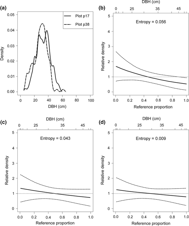
Decomposing the relative distribution of DBH in the plot p17 (cluster no. 6, Gini coefficient = 0.31) and in the plot p38 (cluster no. 6, Gini coefficient = 0.33) into the impact of changes in medians and changes in shape; dashed lines show 95 % confidence intervals. a. Approximation of the empirical DBH data using the kernel density estimator. b Overall relative density. c Location decomposition. d Shape decomposition. DBH is the tree diameter at breast height
-
2.
plot p59 (cluster no. 5; unmanaged stand; the Gini coefficient was 0.51; it was the minimum value for group IV; Fig. 8);
Fig. 8 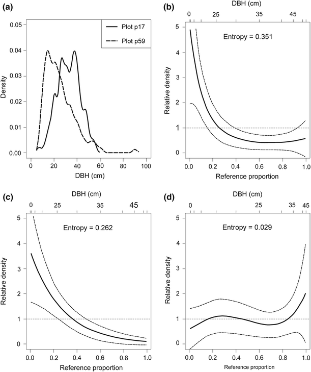
Decomposing the relative distribution of DBH in the plot p17 (cluster no. 6, Gini coefficient = 0.31) and in the plot p59 (cluster no. 5, Gini coefficient = 0.51) into the impact of changes in medians and changes in shape; dashed lines show 95 % confidence intervals. a. Approximation of the empirical DBH data using the kernel density estimator. b Overall relative density. c Location decomposition. d Shape decomposition. DBH is the tree diameter at breast height
-
3.
plot p58 (cluster no. 5; unmanaged stand; the Gini coefficient was 0.58; it was the maximum value for this cluster; Fig. 9).
Fig. 9 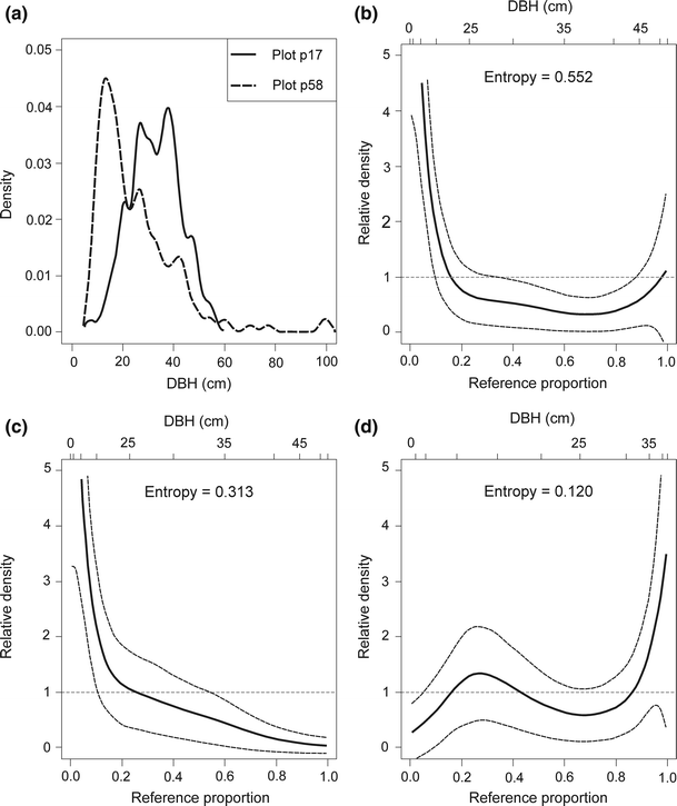
Decomposing the relative distribution of DBH in the plot p17 (cluster no. 6, Gini coefficient = 0.31) and in the plot p58 (cluster no. 5, Gini coefficient = 0.58) into the impact of changes in medians and changes in shape; dashed lines show 95 % confidence intervals. a. Approximation of the empirical DBH data using the kernel density estimator. b Overall relative density. c Location decomposition. d Shape decomposition. DBH is the tree diameter at breast height


The relative density is useful to examine the two basic components which form the differences in location (the median shift) and differences in shape (the shape shift). For the first comparison (plot p17 and p38) the median shift as well as the shape shift were close to zero (the 95 % CIs, indicated by dashed lines, entirely overlap relative density equal to 1; Fig. 7c, d). For the second and third comparisons (plot p17 and p59 as well as plot p17 and p58) the median shifts were significant and the shape shifts were close to zero (the inequality observed in Figs. 8a, 9a were largely a product of median differences; see also Figs. 8c, d, 9c, d). The entropy measures are used to assess overall dispersion between the two distributions. These measures suggest that the median shifts were more important in generating the differences between plot p17 and p59 as well as between plot p17 and p58 (the respective values of entropy were 0.262 and 0.313 for median shift and 0.029 and 0.120 for shape shift). If there is a divergence between distributions, we can test polarisation. For successive comparisons (plot p17 and p38, plot p17 and p59 as well as plot p17 and p58), the MRP polarisation index values were −0.083 (95 % CI was from −0.083 to 0.074), 0.034 (95 % CI was from −0.114 to 0.182) and 0.094 (95 % CI was from −0.057 to 0.244), respectively. All MRP values were not significant and show that polarisation was not occurring for these comparisons. Full distributional comparisons of DBH distributions showed significant differences in location and did not show significant differences in shape between unimodal, similar structural types in managed (cluster no. 6; plot p17) and in unmanaged (cluster no. 5; plots p59 and p58) stands.
The obtained results confirm the third hypothesis that unmanaged forests are characterised by significantly more heterogeneous tree diameter structural diversity compared to managed stands.
Discussion
Structural patterns in stands with A. alba and F. sylvatica
Considering the great importance of A. alba and F. sylvatica in unmanaged as well as managed mountain forests and the dominating role they have in many of Central Europe’s forest ecosystems, studies of DBH structural diversity are surprisingly rare (e.g. Wolf et al. 2004; von Oheimb et al. 2005; Piovesan et al. 2005; Jaworski and Podlaski 2007; Bílek et al. 2011). A. alba and F. sylvatica can grow in stands of heterogeneous size structure, from one-storied through multi-storied to finally selection structure (e.g. Čavlović et al. 2006; Podlaski 2010; Kerr 2014). The most appropriate structure of stand with large share of A. alba is multi-storied or selection structure (uneven-aged stand). In a forest of high vertical diversity that means a high variation of DBH distribution, the biological diversity is larger and more visible than in less structural complex forests (e.g. Spies 1998; Lindenmayer et al. 2000; Moning et al. 2009; Taboada et al. 2010; Sullivan et al. 2013).
In managed stands size structures are formed under the influence of the applied cutting methods and thinnings. In unmanaged stands size structures are shaped by, above all, spatial and temporal gap dynamics and neighbourhood processes occurring between single trees and whole patches. Reverse-J DBH distribution is usually interpreted as a situation where small-scale gap dynamics drive the succession with trees in all sizes at a small scale. The most complex size structures, rotated-sigmoid and bimodal DBH distributions, are produced by three main mechanisms: (1) infrequent disturbance at intermediate and coarse scales, (2) U-shaped mortality, and (3) nonlinear diameter increment (faster in medium-size trees compared to smaller and larger ones) (Leak 2002; Alessandrini et al. 2011).
Tree diameter distribution models in stands with A. alba and F. sylvatica
Empirical DBH distributions in the distinguished structural types were most precisely approximated by single and mixture Weibull and gamma models. The obtained results confirmed the wide applicability of the Weibull and gamma distributions in describing the DBH distributions of mixed stands consisting of A. alba and F. sylvatica. Similar results were also presented by other authors, e.g. Zhang et al. (2001), Liu et al. (2002), Zhang and Liu (2006), Jaworski and Podlaski (2012), Podlaski and Roesch (2014), successfully used a mixture of Weibull and gamma distributions to describe the DBH data of mixed species forests.
For some plots were large differences of tree numbers between neighbouring DBH classes. In the case of the occurrence of this random, local irregularity, goodness of fit test showed a not very precise fit of the investigated models. Such a phenomenon of irregular DBH distribution can be caused by (1) simultaneous occurrence of gaps in forest canopy created by dying trees and seeding year that cover the whole gap with natural regeneration, (2) various diameter growth dynamics of trees growing under diversified light conditions (Nagel et al. 2006). In the first case, all the trees growing in the gaps have similar DBHs and the period of DBH growth depends on the size of the gap. In the second case, the growth of some trees can be suppressed in unfavourable light condition e.g. shaded by larger ones while neighbouring trees growing in better light conditions can indicate normal or even intensified DBH growth. This could create unexpected larger amount of trees in certain DBH classes (Goff and West 1975).
Heterogeneity in managed and unmanaged stands
The Gini coefficient was used in many studies as an objective measure to compare tree size diversity at the stand and/or landscape level. In the case of typical even-aged and uneven-aged stands the Gini coefficient varied from 0.21 to 0.51, with a mean value of 0.38 (Lexerød and Eid 2006). In simulated DBH distributions the Gini coefficient varied from 0.16 to 0.57, with a mean value of 0.40, the range of 0.16–0.30 indicating normal distribution, and the range of 0.44–0.57 indicating reverse-J DBH distribution (Lexerød and Eid 2006). As compared to these values, the DBH differentiation expressed as the Gini coefficient for the investigated plots was high, particularly in the case of unmanaged stands (the maximum value of the Gini coefficient in the Świętokrzyski National Park was 0.73). In general, the Gini coefficient is an index which completely and in a logical way discriminated between different DBH distributions.
The assessment of stand heterogeneity by means of the Gini coefficient is usually based on a sample of individual trees representing the investigated stand. In this case the Gini coefficient is an estimator. It is important to know the statistical properties of the Gini coefficient when it is calculated from a sample. This coefficient will be a biased estimator of the true DBH diversity if the number of trees in a sample is <50. The Gini coefficient has a bias practically equal to zero when the number of trees in a sample is >100, or its value is <0.2 (Weiner and Solbrig 1984; Dixon et al. 1987). The Gini coefficient is an index in the case of which the sensitivity to sample size is considered to be low (Lexerød and Eid 2006).
The relative distribution method can give a more descriptive and intuitively more appealing perspective on comparing distributions. Comparisons can be summarised graphically as well as the used summary statistics can be decomposed by shape and location. A comparison of plot p17 (cluster no. 6) and plot p69 i p58 (cluster no. 5) shows that in spite of a similar shape (the respective shape shifts were close to zero) the analysed empirical DBH distributions differ significantly, taking into account their location (the respective median shifts were significant). It was possible to carry out the analysis of this type because the relative distribution method allows us to rescale the comparison to the referent distribution and the lack of parametric assumptions.
The results of the paper indicate that a more diversified DBH distribution occurs in unmanaged than in managed stands. Different results were obtained by e.g. Kuuluvainen et al. (1996) and Rouvinen and Kuuluvainen (2005), which showed that both unmanaged and managed stands had heterogeneous DBH distributions. The presented differences are connected with forest management methods used in the investigated stands. Cutting methods and thinnings played and still play a significant role in shaping the forest structure. In most papers was stressed a significant difference between the unmanaged and managed stands: the first group is characterised by a higher proportion of live trees in large DBH classes as compared to the other group (e.g. Crow et al. 2002).
Unmanaged forests, where structure is more diversified, are considered to be richer in terms of species and habitat diversity than managed forests (Bobiec 1998; Økland et al. 2003; Tews et al. 2004). One should, however, remember that the properly carried out forest management may positively influence forest biodiversity (Vaisanen et al. 1993; Schmidt 2005; Paillet et al. 2009).
Implications for silviculture and forest management
Silviculture might and should use all possible measures to enhance biodiversity of stands, including all main attributes of biodiversity (composition, structure, and function into a nested hierarchy) (Kerr 1999; Bengtsson et al. 2000; Puettmann and Tappeiner 2014). One of the common means used in managed stands is to follow close-to-nature silviculture that tries to mimic natural processes occurring in unmanaged, natural forests (Lähde et al. 1999; Schütz 1999; Çolak et al. 2003; Gamborg and Larsen 2003). Among different operations taken under close-to-nature silviculture that have influence on biodiversity of stands with A. alba and F. sylvatica are: (1) cutting methods that mimic fine-scale disturbances, (2) more complex reproduction systems with a longer regeneration period, and (3) thinnings.
One of the main attributes of natural processes is the occurrence of disturbances at different spatial scales. As a key component of ecosystem dynamics, disturbances greatly affect the structure, composition and function of forests (Mitchell 2013). In Central Europe disturbances in the form of canopy gaps, very often caused by wind, are crucial for a natural process of stand regeneration (e.g. Nagel and Diaci 2006; Nagel et al. 2006; Dobrowolska and Veblen 2008; Kucbel et al. 2010). In order to ensure adequate structure and natural processes in managed stands, forest management should implement appropriate cutting methods that imitate disturbances, especially at the fine scale which, in the long term, shape multi-layered and multi-aged forests (Long 2009; Mori 2011; O’Hara and Ramage 2013).
The more complex reproduction systems are characterised by, among others, irregular, spatially differentiated cuttings and longer regeneration periods. An example of this way of management is an irregular group shelterwood reproduction method and plenter system (e.g. Boncina 2011; Kerr 2014). As the result of the application of the first silviculture method we obtain irregular uneven-aged patches, while the second method results in the formation of balanced uneven-aged structures. This type of forest management allows one to increase biodiversity because stands characterised by great structural diversity are more favourable for wildlife and hence more stable but only within the limits imposed by site and climate. An additional effect of the application of more complex reproduction systems is multifunctionality of stands (Bagnaresi et al. 2002; Schütz 2002).
Thinnings belong to one of the most important treatments performed during the stand life span, after the establishment of a new stand and prior to the final harvest. To loosen crown cover, to let more light in the stand and to diversify vertical structure of stands, a special method of thinning should be applied that involves the cuttings promoting the best trees in terms of vitality and growth tendency in all layers of stand as well as additionally releases and initiates natural regeneration. It can accelerate recovery of stand structure and species diversity of understory vegetation (Lindh and Muir 2004; Sullivan et al. 2009).
Conclusions
-
1.
In the theory and practice of silviculture and, above all, in forest management the term ‘biodiversity’ should be identified with not only species diversity but also structural diversity. In forest ecosystems biodiversity of all tree layers and forest floor depends to a large extent on tree diameter structural diversity.
-
2.
The present studies have shown that tree diameter structural diversity was more complex in unmanaged forests compared to managed stands.
-
3.
Managed forests, and particularly those composed of shade tolerant species (e.g. A. alba, F. sylvatica), should be characterised by differentiated tree diameter structural diversity. In these forests, one should aim to create not only UMs, but also complex structures: rotated-sigmoid, bimodal and selection DBH distributions.
-
4.
During transformation processes, aimed to increase biodiversity in managed forests, it is necessary to monitor, among others, tree diameter structural diversity.
-
5.
Leaving more trees in large DBH classes allows one to increase tree diameter structural diversity in each DBH structural type.
-
6.
To assess DBH structural diversity, one should use, in addition to different indexes and coefficients, empirical DBH distributions and theoretical models. Especially the description of rotated-sigmoid, bimodal and irregular forms of empirical DBH distributions can be improved using more flexible models. For analyses of DBH structural diversity, strongly recommended are mixture models with Weibull and gamma functions as well as the Gini coefficient and the relative distribution method.
References
Aho K, Winston V, Roberts D (2013) asbio: a collection of statistical tools for biologists. R package version 1.0. http://CRAN.R-project.org/package=asbio
Alessandrini A, Biondi F, Di Filippo A, Ziaco E, Piovesan G (2011) Tree size distribution at increasing spatial scales converges to the rotated sigmoid curve in two old-growth beech stands of the Italian Apennines. For Ecol Manag 262:1950–1962
Bagnaresi U, Giannini R, Grassi G, Minotta G, Paffetti D, Pini Prato E, Proietti Placidi AM (2002) Stand structure and biodiversity in mixed, uneven-aged coniferous forests in the eastern Alps. Forestry 75:357–364
Bengtsson J, Nilsson SG, Franc A, Menozzi P (2000) Biodiversity, disturbances, ecosystem function and management of European forests. For Ecol Manag 132:39–50
Bílek L, Remeš J, Zahradník D (2011) Managed vs. unmanaged. Structure of beech forest stands (Fagus sylvatica L.) after 50 years of development, Central Bohemia. For Syst 20:122–138
Bobiec A (1998) The mosaic diversity of field layer vegetation in the natural and exploited forests of Białowieża. Plant Ecol 136:175–187
Boncina A (2011) History, current status and future prospects of uneven-aged forest management in the Dinaric region: an overview. Forestry 84:467–478
Čavlović J, Božić M, Boncina A (2006) Stand structure of an uneven-aged fir–beech forest with an irregular diameter structure: modeling the development of the Belevine forest, Croatia. Eur J For Res 125:325–333
Ciołkosz A (1991) SINUS—System Informacji o Środowisku Przyrodniczym. In: Mazur S (ed) Ekologiczne Podstawy Gospodarowania Środowiskiem Przyrodniczym. Wizje—problemy—trudności. Wyd. SGGW-AR, Warszawa, pp 317–328
Clarke KR (1993) Non-parametric multivariate analysis of changes in community structure. Aust J Ecol 18:117–143
Cochran WG (1977) Sampling techniques. Wiley, New York
Çolak AH, Rotherham ID, Çalikoglu M (2003) Combining ‘naturalness concepts’ with close-to-nature silviculture. Forstw Cbl 122:421–431
Crow TR, Buckley DS, Nauertz EA, Zasada JC (2002) Effects of management on the composition and structure of northern hardwood forests in Upper Michigan. For Sci 48:129–145
Dixon PM, Weiner J, Mitchell-Olds T, Woodley R (1987) Bootstrapping the Gini coefficient of inequality. Ecology 68:1548–1551
Dobrowolska D, Veblen TT (2008) Treefall-gap structure and regeneration in mixed Abies alba stands in central Poland. For Ecol Manag 255:3469–3476
Dolezal J, Song J-S, Altman J, Janecek S, Cerny T, Srutek M, Kolbek J (2009) Tree growth and competition in a post-logging Quercus mongolica forest on Mt. Sobaek, South Korea. Ecol Res 24:281–290
Faith DP, Minchin PR, Belbin L (1987) Compositional dissimilarity as a robust measure of ecological distance. Vegetatio 69:57–68
FAO, ISRIC, ISSS (2006) World reference base for soil resources (World Soil Resources Reports no. 103). FAO, Rome
Ferris R, Humphrey JW (1999) A review of potential biodiversity indicators for application in British forests. Forestry 72:313–328
Franklin JF, Spies TA, Van Pelt R, Carey AB, Thornburgh DA, Berg DR, Lindenmayer DB, Harmon ME, Keeton WS, Shaw DC, Bible K, Chen J (2002) Disturbances and structural development of natural forest ecosystems with silvicultural implications, using Douglas-Fir forests as an example. For Ecol Manag 155:399–423
Gamborg C, Larsen JB (2003) ‘Back to nature’—a sustainable future for forestry? For Ecol Manag 179:559–571
Gini C (1921) Measurement of inequality on income. Econ J 31:22–43
Goff FG, West D (1975) Canopy–understory interaction effects on forest population structure. For Sci 21:98–108
Gordon AD (1999) Classification, 2nd edn. Chapman and Hall/CRC, London
Gracia M, Montané F, Piqué J, Retana J (2007) Overstory structure and topographic gradients determining diversity and abundance of understory shrub species in temperate forests in central Pyrenees (NE Spain). For Ecol Manag 242:391–397
Handcock MS, Morris M (1999) Relative distribution methods in the social sciences. Springer, New York
Hansen AJ, Garman SL, Weugand JF, Urban DL, McComb WC, Raphael MG (1995) Alternative silvicultural regimes in the Pacific Northwest: simulations of ecological and economic effects. Ecol Appl 5:535–554
Hartigan JA (1975) Clustering algorithms. Wiley, New York
Hubbell SP, Ahumada JA, Condit R, Foster RB (2001) Local neighborhood effects on long-term survival of individual trees in a neotropical forest. Ecol Res 16:859–875
Jaworski A (1982) Fir regression in Polish mountain areas. Eur J For Pathol 12:143–149
Jaworski A, Podlaski R (2007) Structure and dynamics of selected stands of primeval character in the Pieniny National Park. Dendrobiology 58:25–42
Jaworski A, Podlaski R (2012) Modelling irregular and multimodal tree diameter distributions by finite mixture models: an approach to stand structure characterization. J For Res 17:79–88
Jukes MR, Ferris R, Peace AJ (2002) The influence of stand structure and composition on diversity of canopy Coleoptera in coniferous plantations in Britain. For Ecol Manag 163:27–41
Kato J, Hayashi I (2007) Quantitative analysis of a stand of Pinus densiflora undergoing succession to Quercus mongolica ssp crispula: II. Growth and population dynamics of Q. mongolica ssp. crispula under the P. densiflora canopy. Ecol Res 22:527–533
Kerr G (1999) The use of silvicultural systems to enhance biological diversity of plantation forests in Britain. Forestry 72:191–205
Kerr G (2014) The management of silver fir forests: de Liocourt (1898) revisited. Forestry 87:29–38
Kucbel S, Jaloviar P, Saniga M, Vencurik J, Klimaš V (2010) Canopy gaps in an old-growth fir–beech forest remnant of Western Carpathians. Eur J For Res 129:249–259
Kutner MH, Nachtsheim CJ, Neter J, Li W (2005) Applied linear statistical models. McGraw-Hill, Boston
Kuuluvainen T, Penttinen A, Leinonen K, Nygren M (1996) Statistical opportunities for comparing stand structural heterogeneity in managed and primeval forests: an example from boreal spruce forest in southern Finland. Silva Fenn 30:315–328
Lähde E, Laiho O, Norokorpi Y (1999) Diversity-oriented silviculture in the boreal zone of Europe. For Ecol Manag 118:223–243
Leak WB (2002) Origin of sigmoid diameter distributions. Research Paper NE-718. Newtown Square, PA: U.S. Department of Agriculture, Forest Service, Northeastern Research Station
Legendre P, Legendre L (2012) Numerical ecology, 3rd English edition edn. Elsevier Science BV, Amsterdam
Lexerød NL, Eid T (2006) An evaluation of different diameter diversity indices based on criteria related to forest management planning. For Ecol Manag 222:17–28
Lindenmayer DB, Margules CR, Botkin DB (2000) Indicators of biodiversity for ecologically sustainable forest management. Conserv Biol 14:941–950
Lindh BC, Muir PS (2004) Understory vegetation in young Douglas-fir forests: does thinning help restore old-growth composition? For Ecol Manag 192:285–296
Liu C, Zhang L, Davis CJ, Solomon DS, Grove JH (2002) A finite mixture model for characterizing the diameter distribution of mixed-species forest stands. For Sci 48:653–661
Long JN (2009) Emulating natural disturbance regimes as a basis for forest management: a North American view. For Ecol Manag 257:1868–1873
Macdonald P, Du J (2012) mixdist: finite mixture distribution models. R package version 0.5-4. http://CRAN.R-project.org/package=mixdist
Macdonald PDM, Pitcher TJ (1979) Age-groups from size-frequency data: a versatile and efficient method of analyzing distribution mixtures. J Fish Res Board Can 36:987–1001
Matuszkiewicz JM (2008) Zespoły leśne Polski. Państwowe Wydawnictwo Naukowe, Warszawa
McLachlan GJ, Krishnan T (2008) The EM algorithm and extensions. Wiley, Hoboken
Mielke P (1984) Meteorological applications of permutation techniques based on distance functions. In: Krishnaiah PR, Sen PK (eds) Handbook of statistics. North Holland, Amsterdam, pp 813–830
Mielke P (1991) The application of multivariate permutation methods based on distance functions in the earth sciences. Earth-Sci Rev 31:55–71
Mitchell SJ (2013) Wind as a natural disturbance agent in forests: a synthesis. Forestry 86:147–157
Moning C, Werth S, Dziock F, Bässler C, Bradtka J, Hothorn T, Müller J (2009) Lichen diversity in temperate montane forests is influenced by forest structure more than climate. For Ecol Manag 258:745–751
Mori AS (2011) Ecosystem management based on natural disturbances: hierarchical context and non-equilibrium paradigm. J Appl Ecol 48:280–292
Nagel TA, Diaci J (2006) Intermediate wind disturbance in an old-growth beech–fir forest in southeastern Slovenia. Can J For Res 36:629–638
Nagel TA, Svoboda M, Diaci J (2006) Regeneration patterns after intermediate wind disturbance in an old-growth Fagus–Abies forest in southeastern Slovenia. For Ecol Manag 226:268–278
Noss RF (1990) Indicators for monitoring biodiversity: a hierarchical approach. Conserv Biol 4:355–364
O’Hara KL, Ramage BS (2013) Silviculture in an uncertain world: utilizing multi-aged management systems to integrate disturbance. Forestry 86:401–410
Obrębska-Starklowa B, Hess M, Olecki Z, Trepińska J, Kowanetz L (1995) Klimat. In: Warszyńska J (ed) Karpaty Polskie. Przyroda, człowiek i jego działalność. UJ, Kraków, pp 31–47
Økland T, Rydgren K, Økland RH, Storaunet KO, Rolstad J (2003) Variation in environmental conditions, understorey species number, abundance and composition among natural and managed Picea abies forest stands. For Ecol Manag 177:17–37
Oksanen J, Blanchet FG, Kindt R, Legendre P, Minchin PR, O’Hara RB, Simpson GL, Solymos P, Henry M, Stevens H, Wagner H (2013) vegan: community ecology package. R package version 2.0-10. http://CRAN.R-project.org/package=vegan
Olszewski JL, Szałach G, Żarnowiecki G (2000) Klimat. In: Cieśliński S, Kowalkowski A (eds) Świętokrzyski Park Narodowy. Przyroda, Gospodarka, Kultura. Świętokrzyski Park Narodowy, Bodzentyn, pp 129–145
Paillet Y, Bergès L, Hjältén J, Ódor P, Avon C, Bernhardt-Römermann M, Bijlsma R-J, de Bruyn L, Fuhr M, Grandin U, Kanka R, Lundin L, Luque S, Magura T, Matesanz S, Mészáros I, Sebastià M-T, Schmidt W, Standovár T, Tóthmérész B, Uotila A, Valladares F, Vellak K, Virtanen R (2009) Biodiversity differences between managed and unmanaged forests: meta-analysis of species richness in Europe. Conserv Biol 24:101–112
Parzen E (1962) On estimation of the probability density function and mode. Ann Math Stat 33:1056–1076
Piovesan G, Di Fillipo A, Alessandrini A, Biondi F, Schirone B (2005) Structure, dynamics and dendroecology of an old-growth Fagus forest in the Apennines. J Veg Sci 16:13–28
Podlaski R (2005) Inventory of the degree of tree defoliation in small areas. For Ecol Manag 215:361–377
Podlaski R (2010) Diversity of patch structure in Central European forests: are tree diameter distributions in near-natural multilayered Abies–Fagus stands heterogeneous? Ecol Res 25:599–608
Podlaski R (2011a) Modelowanie rozkładów pierśnic drzew z wykorzystaniem rozkładów mieszanych. I. Rozkłady mieszane: definicja, charakterystyka, estymacja parametrów. Sylwan 155:244–252
Podlaski R (2011b) Modelowanie rozkładów pierśnic drzew z wykorzystaniem rozkładów mieszanych. II. Aproksymacja rozkładów pierśnic w lasach wielopiętrowych. Sylwan 155:293–300
Podlaski R, Roesch FA (2014) Modelling diameter distributions of two-cohort forest stands with various proportions of dominant species: a two-component mixture model approach. Math Biosci 249:60–74
Podlaski R, Zasada M (2008) Comparison of selected statistical distributions for modelling the diameter distributions in nearnatural Abies–Fagus forests in the Świętokrzyski National Park (Poland). Eur J For Res 127:455–463
Pommerening A, Murphy ST (2004) A review of the history, definitions and methods of continuous cover forestry with special attention to afforestation and restocking. Forestry 77:27–44
Puettmann KJ, Tappeiner JC (2014) Multi-scale assessments highlight silvicultural opportunities to increase species diversity and spatial variability in forests. Forestry 87:1–10
Puettmann KJ, Coates KD, Messier C (2009) A critique of silviculture. Managing for complexity. Island Press, Washington
R Core Team (2013) R: a language and environment for statistical computing. R Foundation for Statistical Computing, Vienna, Austria. URL http://www.R-project.org
Reynolds MR, Burk T, Huang W-H (1988) Goodness-of-fit tests and model selection procedures for diameter distribution models. For Sci 34:373–399
Rosenblatt M (1956) Remarks on some nonparametric estimates of a density function. Ann Math Stat 27:832–837
Rosenvald R, Lõhmus A, Kraut A, Remm L (2011) Bird communities in hemiboreal old-growth forests: the roles of food supply, stand structure, and site type. For Ecol Manag 262:1541–1550
Rouvinen S, Kuuluvainen T (2005) Tree diameter distributions in natural and managed old Pinus sylvestris-dominated forests. For Ecol Manag 208:45–61
Schmidt W (2005) Herb layer species as indicators of biodiversity of managed and unmanaged beech forests. For Snow Landsc Res 79:111–125
Schütz JP (1999) Close-to-nature silviculture: is this concept compatible with species diversity? Forestry 72:359–366
Schütz JP (2002) Silviculture tools to develop irregular and diverse forest structures. Forestry 75:329–337
Spiecker H, Mielikäinen K, Köhl M, Skovsgaard JP (1996a) Discussion. In: Spiecker H, Mielikäinen K, Köhl M, Skovsgaard JP (eds) Growth trends in European forests. Springer, Berlin, pp 355–367
Spiecker H, Mielikäinen K, Köhl M, Skovsgaard JP (1996b) Conclusions and summary. In: Spiecker H, Mielikäinen K, Köhl M, Skovsgaard JP (eds) Growth trends in European forests. Springer, Berlin, pp 369–372
Spies TA (1998) Forest structure: a key to the ecosystem. Northwest Sci 72:34–39
Sterba H (2008) Diversity indices based on angle count sampling and their interrelationships when used in forest inventories. Forestry 81:587–597
Sullivan TP, Sullivan DS, Lindgren PMF, Ransome DB (2009) Stand structure and the abundance and diversity of plants and small mammals in natural and intensively managed forests. For Ecol Manag 258:127–141
Sullivan TP, Sullivan DS, Lindgren PMF, Ransome DB (2013) Stand structure and small mammals in intensively managed forests: scale, time, and testing extremes. For Ecol Manag 310:1071–1087
Summers RW, Mavor RA, MacLennan AM, Rebecca GW (1999) The structure of ancient native pinewoods and other woodlands in the Highlands of Scotland. For Ecol Manag 119:231–245
Taboada A, Tárrega R, Calvo L, Marcos E, Marcos JA, Salgado JM (2010) Plant and carabid beetle species diversity in relation to forest type and structural heterogeneity. Eur J For Res 129:31–45
Tews J, Brose U, Grimm V, Tielbörger K, Wichmann MC, Schwager M, Jeltsch F (2004) Animal species diversity driven by habitat heterogeneity/diversity: the importance of keystone structures. J Biogeogr 31:79–92
Theil H, Laitinen K (1980) Singular moment matrices in applied econometrics. In: Krishnaiah PR (ed) Multivariate analysis, vol V. Amsterdam, North Holland, pp 629–649
Vaisanen R, Bistrom O, Heliovaara K (1993) Sub-cortical Coleoptera in dead pines and spruces—is primeval species composition maintained in managed forests? Biodivers Conserv 2:95–113
von Oheimb G, Westphal C, Tempel H, Härdtle W (2005) Structural pattern of nearnatural beech forest (Fagus sylvatica) (Serrahn, North-east Germany). For Ecol Manag 212:253–263
Warton DI, Wright TW, Wang Y (2012) Distance-based multivariate analyses confound location and dispersion effects. Methods Ecol Evol 3:89–101
Weiner J, Solbrig OT (1984) The meaning and measurement of size hierarchies in plant populations. Oecologia 61:334–336
Westphal C, Tremer N, von Oheimb G, Hansen J, von Gadow K, Härdtle W (2006) Is the reverse J-shaped diameter distribution universally applicable in European virgin beech forests? For Ecol Manag 223:75–83
Wolf A, Møller PF, Bradshaw RHW, Bigler J (2004) Storm damage and long-term mortality in a semi-natural, temperate deciduous forest. For Ecol Manag 188:197–210
Zhang L, Liu C (2006) Fitting irregular diameter distributions of forest stands by Weibull, modified Weibull, and mixture Weibull models. J For Res 11:369–372
Zhang LJ, Gove JH, Liu C, Leak WB (2001) A finite mixture of two Weibull distributions for modeling the diameter distributions of rotated-sigmoid, uneven-aged stands. Can J For Res 31:1654–1659
Acknowledgments
We thank the editors and the anonymous reviewers for constructive comments, suggestions and corrections.
Author information
Authors and Affiliations
Corresponding author
Rights and permissions
This article is published under an open access license. Please check the 'Copyright Information' section either on this page or in the PDF for details of this license and what re-use is permitted. If your intended use exceeds what is permitted by the license or if you are unable to locate the licence and re-use information, please contact the Rights and Permissions team.
About this article

Cite this article
Pach, M., Podlaski, R. Tree diameter structural diversity in Central European forests with Abies alba and Fagus sylvatica: managed versus unmanaged forest stands. Ecol Res 30, 367–384 (2015). https://doi.org/10.1007/s11284-014-1232-4
Received:
Accepted:
Published:
Issue Date:
DOI: https://doi.org/10.1007/s11284-014-1232-4