
Abstract
Implementing complex algorithms for big data, artificial intelligence, and graph processing requires enormous effort. Succinct, declarative programs to solve complex problems that can be efficiently executed for batching and streaming data are in demand. This paper presents Nexus, a distributed Datalog evaluation system. It evaluates Datalog programs using the semi-naive algorithm for batch and streaming data using incremental and asynchronous iteration. Furthermore, we evaluate Datalog programs with aggregates to determine the advantages of implementing the semi-naive algorithm using incremental iteration on its performance. Our experimental results show that Nexus significantly outperforms acyclic dataflow-based systems.
1 Introduction
Executing recursive algorithms (such as Connected Components, Finding Shortest Path, PageRank) on large-scale (static or continuous) datasets is essential in graph analytics and artificial intelligence. The need to execute these algorithms efficiently attracts programmers to distributed analytics frameworks, such as Flink [10] and Spark [39], to execute their programs on distributed, scalable clusters of machines.
Yet, expressing recursive algorithms in these frameworks is cumbersome. Systems such as BigDatalog [33], Distributed SociaLite [32], and Myria [36] aim at addressing this issue by providing a declarative way to perform analytics. However, due to inherent problems in their underlying platforms, efficiency is not achieved. For instance, BigDatalog suffers from scheduling overhead while Myria and Socialite from shuffling overhead to carry out iterative computation. Therefore, we still need a system that offers high-level, declarative language support and at the same time can carry out complex analytic tasks on static and continuous datasets efficiently and succinctly.
Recently, we proposed Cog [20] to tackle this problem. Cog is a Datalog’s recursive program evaluation system that implements a semi-naive algorithm [3] in a cyclic dataflow system (namely Apache Flink [10]) using its incremental iterations. Figure 1 shows a performance comparison between Cog and BigDatalog for the Reachability program (given in Listing 14). As we can observe, Cog is 3.8 × faster than BigDatalog. This shows the power of executing cyclic dataflow-based programs instead of acyclic ones (such as Spark’s programs). The reader might think of simply using Flink instead of BigDatalog. Although using Flink would indeed match Cog’s performance, it would lose Cog’s declarativeness: We implemented the Reachability program in only 2 lines of code in Cog, instead of 25 lines for Flink’s DataSet API.

Evaluation result comparison using Reachability program (given in Listing 14)
However, despite the high performance and declarativeness benefits of Cog, it does not support common complex data analytics, such as PageRank, All-Pairs Shortest Path, Connected Components, and Triangle Count. This is because Cog does not support recursive aggregates. Furthermore, Cog cannot be used in streaming scenarios, which are quickly becoming the de-facto setting for many data analytics today [22]. Tackling these two problems is challenging for several reasons. First, optimization is required to evaluate recursive aggregate programs efficiently and in a scalable way. Second, evaluation of recursive aggregates must provide correct results while maintaining efficiency (e.g., avoiding redundant computation). Third, evaluation of recursive queries for streaming workloads should yield high throughput. Fourth, understanding recursive aggregate programs (its transformations and intermediate results) is far from being simple: capturing and storing provenance information requires enormous space in RAM and on disk.
We present Nexus, a Datalog evaluation system that overcomes all the aforementioned challenges. Nexus uses Flink’s delta iterations to efficiently evaluate recursive aggregates. It also leverages Flink’s asynchronous iterations in combination with Flink’s native streaming to achieve real-time analytics. Although Nexus is applicable to general-purpose data analytic tasks on relational datasets, we particularly focus on iterative graph algorithms. In addition, Nexus provides debugging capabilities to understand recursive aggregate programs as well as to explain the outcomes of their derivations. Nexus is an extension of Cog [20]. It comes with a number of new and novel features. In summary, in this paper, we make the following contributions:
-
We propose Nexus to support recursive and non-recursive aggregates for the batch datasets to execute Datalog programs containing aggregations. To implement recursive aggregates, we implement the semi-naive algorithm using Flink’s delta iteration. After each iteration step execution, a lower (for min aggregate) or a higher (for aggregates like max) value is produced for each groupby key.
-
We devise an approach to support Datalog on continuous data streams. We perform continuous evaluation of Datalog programs using Flink’s asynchronous iterations. This implementation also helps in avoiding barrier synchronization overhead. When evaluating, we union tuples generated in both non-recursive and recursive rules. Then, we partition by all the fields, and store values against the partitioned key in a hash table. The evaluation happens continuously.
-
We devise a provenance technique for recursive aggregate programs to support their easy debugging (i.e., output reproduction) and interpretation. Our data provenance technique stores tuples that contribute to recursive rules in a hash table. It also creates a new hash table to store tuples derived in each iteration (i.e., differentials), where each tuple stores a reference to the indexes of its parent tuples as value. We map each hash table to a linear data structure (i.e., array) for constant-time look-ups.
-
We exhaustively benchmark Nexus using five common graph analytics tasks (including two programs that contain aggregation in recursion) with synthetic and real-world datasets. We compare Nexus to acyclic dataflow-based BigDatalog [33] and to Cog [20]. The results show that Nexus is up to 5.5 × faster than the baseline BigDatalog and 3 × faster than Cog. Furthermore, Nexus achieves nearly linear scalability.
Paper Organization
The rest of the paper is organized as follows. Section 2 briefly discusses the background needed to understand the contribution made in this paper. Section 3 gives an overview of the components of our system. Section 4 gives details of our system and describes how Datalog queries are compiled and executed. We also explain the semi-naive evaluation for the streaming case. In Section 5, we describe how we implemented aggregates (recursive aggregates in particular) in our system. We, then, explain how we capture provenance information in Section 6. We evaluate the performance of our system in Section 7. We review related work in Section 8. Finally, we conclude and provide a future outlook in Section 9.
2 Background
We start by providing a brief overview of the Datalog language (including recursion and aggregations) and Apache Flink. Then, we discuss how Flink is suitable for efficient evaluation of Datalog queries for batch and stream processing.
2.1 Datalog
Datalog [11] is a query language based on the logic programming paradigm [23]. Datalog programs consist of rules and operate on facts. A fact is a tuple in a relation. A rule is a sentence that infers facts from others facts. Each rule has the form h :- b1,...,bn, where h is the head predicate of the rule, and each bi is a body predicate separated by a comma “,”, which represents the logical and (∧). A predicate is also known as a relation. Datalog allows us to define recursive rules. A Datalog rule is recursive if the head predicate of a rule also appears in the body of the rule. The facts produced by a rule’s body are written to its head predicate. A relation that comes into existence as a result of a rule execution is called an intensional database (IDB) predicate. A stored relation is called an extensional database (EDB) predicate. As an example, Listing 1 shows the Transitive Closure (TC) program implemented in Datalog. The rule r1 is referred to as an exit rule. The rule r2 is a recursive rule as it has the predicate tc in its head and body. A join is created between the tc and arc predicates in rule r2, and the resulting facts are written to tc head predicate.

Transitive Closure (TC) program in Datalog
Numerous techniques [3, 4, 35] exist to evaluate Datalog programs. Among others, the semi-naive evaluation [3] is notable for its efficiency. Semi-naive evaluation avoids redundant computation by producing facts using only the ones derived in the previous iteration. The final result is obtained by performing a union of the facts produced in all the iterations.
Aggregates
Datalog supports grouped aggregations similarly to SQL, but with a terser syntax:
where the head predicate h has X1,...,Xk group-by term(s) (i.e., the grouping key) and agg() aggregate function(s) (e.g., max) that takes the aggregate term(s) T. The P1(X1,...Xk,T1,...,Tn),... is the body predicate(s). Recursive aggregates are the ones that appear in the head of a recursive rule, whereas non-recursive aggregates appear in the head of a non-recursive rule.
Seo et al. [31] (SociaLite) prove that semi-naive evaluation can be applied to a recursive rule that involves aggregation, under certain conditions. Specifically, they showed that this is possible when the aggregation is a meet operation and the rest of the recursive rule is monotonic under the partial order induced by the meet operation. We will explain this further in Section 5. Recursive aggregates enable users to conveniently and succinctly express graph algorithms. We demonstrate this by providing the Connected Components (CC) program (Listing 2) in Datalog as an example. The hcc IDB predicate consists of pairs of node IDs and labels. At the end of the evaluation, each node will be labeled by the ID of the component that it belongs to. Component IDs are a subset of node IDs. The labels are initialized by r1 to be the node ID itself. Then, rule r2 is the recursive aggregate rule, which propagates labels to neighboring vertices. The rule body of r2 finds node IDs (Y) a particular node (X) is connected to, and propagates the Z label to it. The head predicate hcc of r2 uses the min aggregate function on Z and groups by Y, i.e., it computes the minimum of the propagated labels to each node in each iteration. Note that r2 is a recursive rule, since the hcc predicate appears in both the head and the body. After the evaluation of the recursive rule is finished, rule r3 then counts the distinct component IDs (by using countd).

Connected Components (CC) program in Datalog
Running Example
We demonstrate the semi-naive evaluation of the Connected Components (CC) program (given in Listing 2) with the facts provided in Listing 3.

EDB predicate for the CC program: each line is a separate component
In r1 (a.k.a. exit rule), the facts from the arc EDB predicate are read and five facts are derived and stored in the hcc IDB predicate (Listing 4).

Evaluation of r1 of the CC program
In iteration 1 (Listing 5), the body of the r2 rule produces 5 facts that satisfy the join condition, and the head predicate computes the lowest label value seen so far for each group. Listing 5 shows that hcc(4,3), hcc(6,5), and hcc(8,7) are newly generated facts and hcc(2,1), hcc(3,2) update the labels for the "2" and "3" nodes.

Evaluation of r2 of CC program in iteration 1
In iteration 2, the body of rule r2 creates a join between the facts derived in the previous iteration with arc. The join produces two facts and the head predicate replaces the existing values for groups "3" and "4" with lower values it computed. Listing 6 shows derivations of facts in iteration 2.

Evaluation of r2 of CC program in iteration 2
In iteration 3, the body of r2 produces one fact and the head predicate replaces the existing values for group "4" with a lower value. Listing ?? shows derivations of facts in iteration 3.

Evaluation of r2 of CC program in iteration 3
Listing 8 shows the values stored in hcc IDB. Finally, the non-recursive aggregate countd counts the distinct values of Y in rule r3 and produces "3" as the result of the program.

Facts in the hcc predicate after the evaluation of the CC program
2.2 Apache Flink
Apache Flink [10] is an open-source distributed dataflow system that provides a unified execution engine for batch and stream processing. Compared to other well-known dataflow systems, such as Spark, Flink is notable for iterative processing through cyclic dataflows and for efficient stream processing.
A Flink user writes a program that consists of transformation operators (such as map, filter, and join): the transformation operators take tuples as input, perform operations on the tuples, and produce output. Flink
connects the operators and creates a dataflow graph for the user program. The dataflow graph is a directed cyclic graph of stateful operators connected with data streams which is then executed by Flink’s runtime engine. The data are fed to the program through the source operators and the results are stored by the sink operators. Flink has the DataSet API for batch processing and the DataStream API for stream processing. We will briefly discuss the two APIs.
Stream Processing in Apache Flink
Flink allows for processing unbounded collections of elements through its DataStream API, which is implemented on top of the Flink runtime. DataStream offers typical data transformation operators (such as map, filter, aggregate, joins), source and sink operators. Particularly to stream processing, Flink implemented the notion of time via watermarks and windowing. The watermarking assists in processing events in the correct order. The windowing allows for incremental computations on a subset of unbounded streams. In this paper, we will not use watermarking and windowing and leave these for future work. Furthermore, the DataStream API provides stateful operators where state for each operator is updated continuously. Importantly, Flink provides asynchronous iterations for the streaming tasks. We will discuss Flink’s iterations later in this section.
Batch Processing in Apache Flink
Batch processing can be considered a special case of streaming, where the stream has a specific end point, i.e., it is finite. Apache Flink provides the DataSet API for bounded immutable collections of elements. Similar to the DataStream API, the DataSet API also provides transformations, source and sinks operators. Since the DataSet is a immutable collection of objects, each transformation operator creates a new DataSet after processing its input(s). DataSet-based programs are evaluated lazily, i.e., most DataSet methods just add a node to the dataflow graph, and the dataflow graph is executed when the user program calls an action (e.g., count, collect, print).
Iterations in Flink
Flink’s DataSet API supports two types of iterations: bulk and delta iterations. Bulk iterations compute a completely new result from the previous iteration’s result [14]. Whereas, delta iterations (a type of incremental iteration) produce results that is only partially different from the one computed in the previous iteration. The delta iterations are useful for iterative algorithms with sparse computational dependencies where one iteration affects few data points.
Flink iterations (both bulk and delta) execute a step function in each iteration. The step function consists of a graph of Flink operators. The result of the step function is fed as input via a feedback edge to the next iteration. At the end of each iteration, Flink performs barrier synchronization, i.e. Flink waits for all workers to complete the execution of the step function before starting the next iteration. The barrier synchronization is performed for the batch case (i.e., DataSet API). When using the DataStream API, Flink allows for asynchronous iterations, i.e. not having barrier synchronization. This makes it more efficient by avoiding the synchronization overhead.
Iteration Execution in Cyclic Dataflow Jobs
Flink executes iterative programs written using its iteration APIs in a single, cyclic dataflow job, i.e., where an iteration’s result is fed back as the next iteration’s input through a backwards dataflow edge. Whereas, acyclic dataflow systems, such as Apache Spark [39], execute iterative programs as a series of acyclic dataflow jobs. Flink’s cyclic dataflows are more efficient for several reasons:
-
With a cyclic dataflow job, Flink avoids overhead of scheduling the tasks of the job to a large cluster of machines. In contrast, launching the tasks of an acyclic dataflow job (e.g., in Spark) presents a significant scheduling overhead.
-
Operator lifespans can be extended to all iterations. (Whereas in Spark, new operators are launched for each iteration.) This enables Flink to naturally perform two optimizations:
-
Flink’s delta iteration maintains the solution set in the operator’s state that is extended to all iterations. The solution set is updated in each iteration by adding deltas to it.
-
Flink’s iterations can efficiently reuse loop-invariant datasets, i.e., datasets that are reused without changes in each iteration (e.g., arc in Figure 1). For instance, when one input of a join is a loop-invariant dataset, the join operator can build a hash table of the loop-invariant input only once, and just probe the same hash table in all iterations.
-
3 Overview
We present Nexus, which evaluates Datalog programs that can contain recursive rules and aggregations on a distributed cluster of machines. We start by giving an architectural overview of our system as well as its integration with Apache Flink. Our system’s core objective is to provide a declarative, succinct interface so that users can perform complex analytic tasks that contain recursions and aggregations. Our system takes a Flink program containing Datalog rules as a string and converts it to a Flink job through a series of intermediate steps. The following components perform the intermediate steps to convert a Datalog program to a dataflow job: Parser, Predicate Connection Graph (PCG) generator, Logical planner, and Flink planner. Figure 2 illustrates these components of our system. The parsing, PCG creation, and logical planning are API (i.e., Flink’s DataSet and DataStream APIs) agnostic steps. Flink planner, however, creates DataSet- or DataStream-based plan depending on the execution environment being used.

System overview of Nexus
The parser, based on ANTLR4 [28], parses the input Datalog program, performs syntax validation, and outputs the parse tree for the program. The parse tree is input to the PCG generator that generates the PCG to represent the input program conveniently. The logical planner creates a logical plan from the created PCG by traversing it in a depth-first manner. We used Apache Calcite [6] to create the logical plans. The logical plan is optimized using Flink’s existing volcano planner. The Flink planner creates Flink-based plan for the DataSet or DataStream API, depending upon the execution environment being used. For Flink-based plans, we utilize existing Flink operators; however, we created the repeat union, table spool, and transient scan operators for simple recursive programs and recursive aggregate programs.
4 From datalog to dataflow
We start discussing the main components of our system and detailing the transition from Datalog to dataflow programs consisting of Flink operators.
4.1 Intermediate representation and planning
A Datalog program written in Nexus goes through two steps (query compilation and logical planning) for effective representation and optimization: (1) a parsed program is converted into a Predicate Connection Graph (PCG), and (2) a logical plan is created from the PCG and standard relational algebra optimizations are performed. We now discuss these two steps in detail.
Query Compilation
A parsed Datalog program is represented in the form of a Predicate Connection Graph (PCG) that was introduced for the deductive database system LDL++ [2]. A PCG is an annotated AND/OR tree, i.e., it has alternating levels of AND and OR nodes: The AND nodes represent head predicates of rules; The OR nodes represent body predicates of rules. Thus, the root and the leaves are always OR nodes: While the root of the tree represents the query predicate, the leaf nodes represent body predicates. An AND node can have the recursive flag to identify if the node represents the head predicate of a recursive rule. Figure 3 shows the PCG for the connected components (CC) query (Listing 2) as an example. Note that aggregates are represented as terms in the AND nodes, which represent the head rules, e.g., min<Z> in Figure 3.

Predicate connection graph for the Connected Components program
Logical Planning and Optimization
The logical planner creates a relational algebra-based logical plan from the PCG to represent Datalog queries. This representation enables us to perform traditional query optimization techniques. To properly integrate our system in Flink’s ecosystem, we utilized the algebra module of Apache Calcite [6] to create logical plans. Calcite provides numerous operators (such as join, project, union) to represent a query with relational algebra. To evaluate recursive Datalog queries, the repeat union operator is crucial. The repeat union operator has two child nodes: seed and iterative. The seed node represents facts generated by non-recursive rule(s), whereas the iterative node represents facts generated by the recursive rule(s). The semantics of the repeat union operator are as follows: it first evaluates the seed node, whose result is the input to the first iteration; then, it repeatedly evaluates the iterative node, using the previous iteration’s result. The evaluation terminates when the result does not change between two iterations. Creating logical plans for recursive aggregate queries is a challenging task as Apache Calcite does not support recursive aggregates. We create logical plans to express recursive aggregate in Calcite by combining the repeat union operator with the standard SQL aggregate operators. The Calcite-based logical plans are then transformed into Flink’s own logical plans. During this transformation, standard relational optimizations are also performed. The volcano optimizer performs these optimizations for the batch and streaming cases. The optimized logical plan is then converted to dataflow graphs, either using Flink’s DataSet- or DataStream-based APIs for batch and stream processing, respectively.
4.2 Semi-naive evaluation using delta iteration
We evaluate recursive Datalog programs using the semi-naive evaluation [3] algorithm implemented using Flink’s delta iteration. Note that here we only discuss recursive Datalog programs without aggregates (we discuss recursive aggregates in Section 5).
As discussed earlier, the semi-naive evaluation algorithm is an ideal candidate to evaluate Datalog programs efficiently. Using this technique, each iteration computes results using only the tuples propagated by the previous iteration, thus avoiding redundant computation. The final result is the union of the differentials produced by each iteration. Algorithm 1 and 2 show the semi-naive evaluation and Flink’s delta iterations, respectively. In these algorithms, seed represents the non-recursive rule(s) (a.k.a. the exit rule), whereas recursive represents a single evaluation of the recursive rule. W is the differential calculated in each iteration, and S stores the final result at the end.


Both algorithms are essentially analogous to each other. The algorithms start with an initial solution set (S) and an initial workset (W ). Then, each iteration computes a differential (D) (which is essentially also the workset for the next iteration in Algorithm 1) that is to be merged into the solution set (Line 7). Note that the merging into the solution set is denoted by  in Algorithm 2, which means that elements whose keys not yet appear in the solution set should be added, and elements which have the same key as an element already in the solution set should override the old element:
  D|key(d) = key(s)}. Note that by choosing the key to be the entire tuple, we make the
  behave as a standard union. We can see that with the following mapping, a Flink Delta Iteration performs exactly the semi-naive evaluation of a Datalog query: S = seed; W = seed; u(S,W) = recursive(W) − S; δ(D,S,W) = D; key(x) = x.
When translating from Nexus logical plans, the semi-naive evaluation is implemented to translate the repeat union operator to DataSet operators. Figure 4 shows the Flink plan for the TC query as an example. We use a CoGroup operation to compute the differential for each iteration, i.e., a set difference of tuples created in the current iteration and the solution set. The work set forwards the computed differential to the next iteration for further computation. The solution set accumulates the output in each iterations. The work set and the solution set are always kept in memory for efficiency. The sync task is a special operator created by Flink to perform barrier synchronization. Note that Flink performs the evaluation lazily upon the call of a sink operator.

The Flink plan for Transitive Closure (TC) program. Some operators are omitted/combined for clarity
4.3 Semi-naive evaluation using asynchronous iteration
Here, we discuss the semi-naive evaluation for Flink’s DataStream API using its asynchronous iterations. In the previous subsection, we discussed the semi-naive algorithm to evaluate Datalog’s recursive programs using Flink’s delta iteration for Flink’s DataSet API. A drawback of Flink’s delta iteration for the batch case is that barrier synchronization (i.e., waiting for all workers to complete the tasks of the current iteration) is needed after each iteration. The barrier synchronization affects the system’s performance, especially under the presence of straggler nodes. This is because the workers that complete their tasks early must wait for the others to finish. This is why asynchronous iterations become important to circumvent the barrier synchronization overhead. It is worth noting that the DataStream-based implementation of semi-naive algorithm can also be used for batch (i.e., finite) datasets. By doing so, we avoid barrier synchronization overhead and achieve more efficiency (compared to our DataSet-based implementation) when used with batch datasets.
Using asynchronous iterations to evaluate iterative programs is a challenging task, because, unlike the delta iterations of Flink, asynchronous iterations (which is needed to evaluate iterative tasks on streaming data) do not share similarity with the semi-naive algorithm. Therefore, our implementation technique differs from the one discussed for delta iterations. To implement the semi-naive evaluation algorithm using asynchronous iterations, we create the repeat union operator for the DataStream-API. Listing 9 shows a code snippet of our implementation (based on Algorithm 1). The delta D (corresponds to Line 5 of Algorithm 1) is calculated by: a) taking the union of the tuples generated by the seed and iterative nodes, b) partitioning tuples using all the fields (i.e., Row) as the key, c) storing the tuples as values against the partitioning key (the hash table serves as the solution set). Tuples that require further processing are sent via a feedback edge and a temporary table represents the tuples transmitted through the feedback edge. Finally, the resulting dataflow graph (created with the code in Listing 9) with asynchronous iteration for the TC query is shown in Figure 5.

An implementation of the semi-naive Datalog evaluation algorithm in Flink for the DataStream API using asynchronous iterations. We mapped the algorithm to just a few standard Flink API calls for simplicity

The Flink streaming plan for the Transitive Closure (TC) program. Some operators are omitted/combined for clarity
Note that, thus far, we do not use any streaming-specific operators (such as windowing) in our implementation for the sake of simplicity.
4.4 Limitations in the streaming case
Evaluating Datalog on an infinite stream of data presents a few additional challenges. Over time, the number of input tuples could grow significantly large. A number of operators (such as join or aggregates) must wait until the end of the stream to produce the correct output. Therefore, it is more practical to apply Datalog rules on chunks of data to reduce memory footprint required by the Flink operators. To address this problem, the semantics of windowing in Datalog needs to be added. This addition itself present numerous challenges, which we leave for future work.
5 Aggregates
We now discuss how we evaluate Datalog programs that have aggregations. SociaLite [31] showed that semi-naive evaluation can be used even if the program has an aggregation in a recursive rule, provided that a) the aggregation is a so-called meet operation, i.e., commutative: f(x,y) = f(y,x), associative: f(f(x,y),z) = f(x,f(y,z)) and idempotent: f(x,x) = x, and b) the rest of the recursive rule is monotonic under the partial order induced by the meet operation. If these properties hold, then the semi-naive evaluation converges to the greatest fixed point, and gives the same result as just naively evaluating the recursive rule repeatedly. Common examples for meet operations are min and max, while a counter-example is sum. The partial order induced by min is simply ≤, while max induces ≥.
Transforming logical plans for recursive programs to Flink-based physical plans is a challenging task, because Flink’s delta iteration operator alone is unable to evaluate programs with recursive aggregates. We used standard SQL aggregate functions together with Flink’s delta iteration in the repeat union operator to evaluate recursive aggregate programs. The rest of the paragraph presents our implementation in detail. Algorithm 3 shows the semi-naive evaluation algorithm when aggregation is involved. It differs from Algorithm 1 as follows: After applying the body of the recursive rule, we also apply the aggregation, denoted with aggr(), which groups the tuples and aggregates each group into one tuple (e.g., computes the minimum of each group). Then, we do not simply subtract S, but instead we do a more complicated operation, which we denoted with  . This operation examines the key of each tuple t on its left-hand side, and checks whether a tuple with the same key is already present in the solution set (S). If not, then it simply returns the tuple (which will be added to the solution set in Line 7). If the key is already present in the solution set in a tuple s, then we check whether aggr({t,s}) = s. If yes, then we do not need to replace s with t in the solution set in Line 7, and therefore
  does not return t in Line 5. However, if the equality does not hold, then
  returns t in Line 5 and then
  replaces s with t in Line 7. For example, if the aggregation is min, then we replace a tuple in the solution set if the new value is smaller.

Listing 10 shows the concrete implementation of Algorithm 3. The implementation is somewhat similar to the one we discussed in [21] except for a few differences: a) the groupBy key(s) is the grouping key of the aggregation (instead of using all the fields), and b) coGroup with AggrMinusCoGroupfunction performs the  operation instead of a normal minus.

An implementation of the semi-naive evaluation algorithm in Flink for aggregates evaluation
Note that if an aggregate is used outside of a recursion, then it does not have to be a meet operation. For example, count, sum, and avg can be evaluated efficiently if they are not inside a recursion. As an example, Listing 11 shows the Triangle Count program that contains the count aggregate function. The program proceeds by creating two joins of arc with itself in r1 to find triangles, and then the derived facts are counted in r2. The program finds cliques of size three in the input graph. The algorithm is commonly used in graph analytics, such as community detection [27], motif detection [38], finding graph similarity [29] to name a few.

Triangle Count program in Datalog that contains a count non-recursive aggregate
6 Debugging recursive aggregates via provenance
Datalog programs often contain several recursive aggregate rules. In such a scenario, it is not uncommon to get incorrect program results and hence makes it necessary to debug Datalog programs, especially knowing the provenance of results (data provenance). Yet, the declarative nature of Datalog makes it challenging for users to inspect the different tuple transformations during complex high-level tasks. A simple Datalog program with only a few rules can result in an explosion of transformations in the dataflow. Furthermore, the
dataflow programs (e.g., Flink jobs) are several times bigger than their Datalog program equivalents. For example, the CC Datalog program (see Listing 2) is composed of 3 lines, but results in 15 Flink operators. Debugging and interpreting such programs is notoriously hard. Therefore, it is desired to capture tuple transformations to trace back tuples’ lineage and interpret the transformations. However, capturing data provenance in the presence of recursive aggregate rules is challenging for a couple of reasons. First, there is usually a large number of iterations that significantly increase the size of the data provenance information. Second, a recursive rule might contain numerous operations that make it harder to trace.
We propose a new technique for efficiently capturing data provenance information in Datalog’s recursive aggregate rules. Figure 6 shows our target area for provenance capture in a red rectangle. Our data provenance technique is based on the TagSniff model [13]. In more detail, we flag the start and end of each iteration to prune the operators that should not be involved in provenance. By doing so, we can ignore non-recursive rules, which significantly reduces the number of tuples for which we capture the provenance information. To achieve this, we add non-recursive rules to the workset at the beginning of each iteration. This workset represents the origin of the inputs to each iteration, which allows us to trace back the tuples in workset. Additionally, we ignore post-iteration operators to keep provenance succinct, allowing to further reduce the number of tuples to trace. This means that the tuples in the solution set are regarded as the “output”.

Provenance capture for the recursion part in programs with recursive aggregate
It is worth noting a scenario that can also result in capturing a large amount of data provenance information. Consider a program of the form given in Listing 12. The problem in this example is that the aggregation operators (GroupCombine and GroupReduce) become part of the iteration and this aggregation is performed in each iteration. However, we want to exclude this aggregation, as our assumption is that this rule might be trivial and does not contain any issues, and therefore the user wants to exclude this from provenance. We thus skip such aggregations, reducing further the amount of data provenance information to store as we do not store some intermediate results inside each iteration.

Contrived example program in Datalog for Provenance
To further reduce the amount of stored data provenance information, we build a hash table for the workset and base relation(s) involved in each iteration. This allows us to reference tuples (i.e., differentials) derived during the execution of each iteration. In other words, we build hash tables at each iteration and store the derived tuples. Then, any derived tuple can reference to the tuples in the previous hash tables. To ease look-ups for previous tuples that contributed to the current tuple, we annotate tuples with a flag (i.e., iteration number) if they came from workset or created/modified in any of the previous iterations. We store all hash tables created in iterations in a linear data structure to assist users in interpreting transformations happened between particular iterations. As a result, we can avoid full scan of the hash table when looking for tuples from a particular iteration. When finished capturing provenance, the hash tables will contain exactly the same number of tuples that are derived during iterations along with the number of tuples that are in the base relation(s). As an example, Figure 7 illustrates our technique of provenance capture for the running example of the Connected Components (in Listing 2) program mentioned in Section 2.1.

Provenance capture for the Connected Components (CC) running example (in Section 2.1)
When tracing back, we take tuples from the solution set and trace back to the workset or base relation tuples. The tuples stored in the solution set also contain the iteration number. This help us in determining which iteration created the tuple and we can then start tracing back to workset/base tuples from the hash table in that iteration number. Doing so we can prune many elements when tracing, hence making traversing efficient.
Our data provenance technique store only information for those tuples that are in the workset/base relation(s) and the solution set, with the addition of the references and iteration numbers. The runtime is linear (i.e., up to the total number of iterations) when tracing back a tuple from the solution set to its source. Note that we do not implement provenance capture for aggregations in mutual recursion, negation, and recursive aggregations with asynchronous iterations (i.e., for the streaming case), which we leave to future work.
7 Experiments
We evaluate Nexus to answer the following questions: a) How efficient our system is for recursive queries and recursive aggregates compared to a system based on acyclic dataflow? b) How does asynchronous iteration help in avoiding barrier synchronization overhead present in Flink’s delta iteration? c) What challenges does asynchronous iteration pose in our experiments? d) How well our system scales with the number of machines and with data sizes? To answer these questions, we perform several experiments to measure performance and scalability of our system using the experimental setup we discuss in Section 7.1. For statistical significance, we run our experiments between 5–10 times and report the medians of results, which removes the effect of outliers when present. Note that outliers appear because of data spilling to disks for large datasets. Also note that Nexus can be used to perform general-purpose analytic tasks, we particularly focus on graph analytics in our experiments.
7.1 Experimental setup
Hardware and Software Environment
We perform our experiments on a cluster of 25 nodes, each with 2x8 core AMD Opteron 6128 CPUs, 30GB memory allocated to Spark and Flink processes, connected with Gigabit Ethernet, and running Ubuntu 18.04 OS. For Spark workers, we allocated 0.75 − 0.85 fraction of total executor memory to JVM heap space, 0.45 − 0.65 for storage, and 2g − 5g off-heap memory for our experiments. For Flink task managers, we allocated 4g − 5g off-heap memory, 0.2 − 0.25 fraction of the allocated memory to network buffers for our experiments.
We perform experiments with large (i.e., up to billion of edges) graphs on a larger cluster. The cluster consists of 33 machines (1 master and 32 workers) each equipped with 16 cores Intel Xeon Silver 4216 2.1GHz CPUs, 60GB memory allocated to Spark and Flink processes, connected with Gigabit Ethernet. For Spark workers, we allocated 0.75 − 0.85 fraction of total executor memory to JVM heap space, 0.45 − 0.65 for storage, and 5g − 8g off-heap memory for our experiments. For Flink task managers, we allocated 8g − 12g off-heap memory, 0.25 − 0.3 fraction of the allocated memory to network buffers for our experiments. We used Java 1.8 and Scala 2.11 for the implementation. Furthermore, we implemented Nexus on top of commit 8f8e358(≈ Flink 1.11 version).
Datasets
We used synthetic and real-world graph datasets in our experiments. The synthetic datasets are Tree11, Grid150, and G10K. The same datasets are also used by Shkapsky et al. [33] in their experiments. Table 1 shows the properties of the datasets. These graphs have specific structural properties: Tree11 has 11 levels, Grid150 is a grid of 151 by 151, and the G10K graph is a 10k-vertex random graph in which each randomly-chosen pair of vertices is connected with probability 0.001. The last three columns of Table 1 show the output size produced with these datasets by the benchmark queries. For the Reachability, CC, and SSSP program, we used graph datasets generated with RMAT [43] synthetic graph generator with the following probabilities: (1) a = 0.45,b = 0.25,c = 0.15,d = 0.15; (2) a = 0.25,b = 0.25,c = 0.25,d = 0.25; (3) a = 0.50,b = 0.20,c = 0.10,d = 0.20; and (4) a = 0.35,b = 0.25,c = 0.15,d = 0.25. Furthermore, we perform benchmark comparisons also by using real-world graph datasets. These real-world graph datasets include LiveJournal [44] and Orkut [45]. For our experiments with large-scale (i.e., billion-scale) graph datasets, we used Arabic-2005, UK-2005, Twitter-2010, and SK-2005 datasets [7, 8] (Table 2). Table 3 specifies the real-world graph datasets.
Benchmark Programs
We use the following recursive aggregate programs in our experiments. Programs with simple recursive queries: We use the following programs to evaluate the performance of recursive queries of Datalog for the batch and streaming cases. We also use these programs in our scalability experiments.
-
Transitive Closure (TC): Finds all pairs of vertices in a graph that are connected by some path. Figure 1 in Section 5 shows the TC program written in Datalog.
-
Same Generation (SG): Two nodes are in the Same Generation (SG) if and only if they are at the same distance from another node in the graph. Listing 13 shows the SG program written in Datalog. The program finds all pairs that are in the same generation.
-
Single-Source Reachability (Reachability): The program finds all vertices connected by some path to a given source vertex. Listing 14 shows the Reachability program written in Datalog.

Same Generation (SG) program in Datalog

Reachability program in Datalog
Programs with recursive aggregates: We use the following programs to evaluate the performance of recursive aggregate programs for the batch case (i.e., Flink’s DataSet API) only.
-
Connected Components (CC): This program identifies the connected components in a graph. Listing 2 in Section 2.1 shows the CC program written in Datalog.
-
Single-Source Shortest Paths (SSSP): This program operates on a weighted graph, and computes the lengths of the shortest paths from a source vertex to all the connected vertices. Listing 15 shows the SSSP program written in Datalog.
-
PageRank (PageRank): PageRank [9] is a popular graph-based link analysis algorithm that is used to compute the importance of vertices in a graph. It is an iterative algorithm that runs until the specified iteration threshold is reached (unlike the previously mentioned algorithms that run until convergence). Listing 16 shows PageRank program written in Datalog.

Single-Source Shortest Path (SSSP) program in Datalog

PageRank (PageRank) program in Datalog
7.2 Performance
For the batch case, we performed a benchmark comparison of our system with an acyclic dataflow-based system, namely BigDatalog [33]. Shkapsky et al. showed BigDatalog’s superior performance over Myria [36], Socialite [32], GraphX [18], and Spark [39]. We also wanted to perform benchmark comparison with RaSQL [19], but we could not do so due to unavailability of its source code. We also performed benchmark comparison of recursive Datalog programs evaluated using the streaming case with Cog to determine the advantage of avoiding barrier synchronization after each iteration.
Evaluating Recursive Programs
-
1.
Transitive Closure (TC): Figure 8 (the left part) shows the result of our TC experiment on synthetic graph datasets. We observe that Cog outperforms BigDatalog in most of the experiments. Particularly, Cog is 3.1 × faster for the batch case and Nexus is 7.1 × faster for the streaming case when compared to BigDatalog for Grid150 dataset. Cog is 2.3 × faster for the batch case and Nexus is 6.8 × faster for the streaming case when compared to BigDatalog for Tree11 dataset. Nexus (i.e., the streaming case) is 2.9 × faster than Cog (i.e., the batch case) in one of our TC experiments. The streaming implementation of Nexus offers the advantage of asynchronous iteration (i.e., no barrier synchronization) over the Cog’s batch case (i.e., with barrier synchronization). BigDatalog suffers from the scheduling overhead caused by the large number of iterations, whereas no such overhead is present in Nexus as it performs iterative programs in a cyclic dataflow job [16]. This overhead gets worse when we have a large number of iterations (as can be seen when grid150 dataset is used). However, this overhead is negligible when there is only a small number of iterations (see parenthesized iteration number in column 4 of Table 1). We also observe that in the case of G10K Nexus does not have significant performance advantage. This is due to data spilling to disk during the join operation.
-
2.
Same Generation (SG): Figure 8 (the right part) shows the result of SG experiments on the synthetic graph datasets. We observe that, Cog is 2.8 × faster and Nexus is 8.4 × faster than BigDatalog for Grid150 dataset. However, Nexus is only 2.7 × faster than BigDatalog for the G10k dataset. These results show that Nexus is much faster when a larger number of iterations is required for convergence (as is the case with Grid150 for 149 iterations). We also observe that Nexus runs out of memory when executing SG on the Tree11 dataset. The reason for running out of memory is that the solution sets could not fit in memory. Nexus with the DataStream API (i.e., with asynchronous iterations) runs 2.9 × faster than Cog for the Grid150 and 2 × faster for the G10K datasets.
-
3.
Reachability (Reachability): Figures 9, 10, 11, and 12 show the result of our Reachability experiments on the synthetic graph datasets created with various probabilities (as discussed in Section 7.1). We observe that Nexus outperforms BigDatalog in all cases. In many cases, the difference in performance between Nexus and BigDatalog gets more prominent with the increase in the size of the datasets. With 2 × increase in the dataset size, we observe 1.0 − 1.2 × increase in the execution time for Cog, 1.1 − 1.6 × for BigDatalog, and 1.1 − 1.8 × for Nexus for RMAT dataset with configuration 1; 1.0 − 1.3 × increase in the execution time for Cog, 1.4 − 1.5 × for BigDatalog, and 1.2 − 1.4 × for Nexus for RMAT dataset with configuration 2; 1.0 − 1.5 × increase in the execution time for Cog, 1.2 − 1.5 × for BigDatalog, and 1.2 − 1.6 × for Nexus for RMAT dataset with configuration 3; and 1.1 − 1.7 × increase in the execution time for Cog, 1.2 − 1.6 × for BigDatalog, and 1.3 − 1.9 × for Nexus for RMAT dataset with configuration 4.
Figure 8 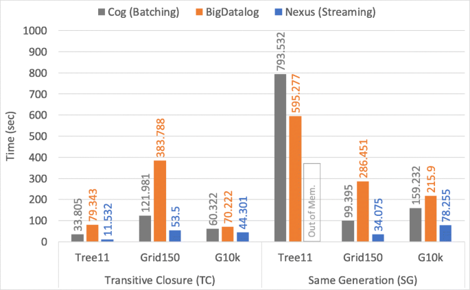
Performance comparison using the TC and SG programs
Figure 9 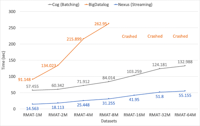
Performance comparison using the Reachability program on different graph sizes (for configuration 1)
Figure 10 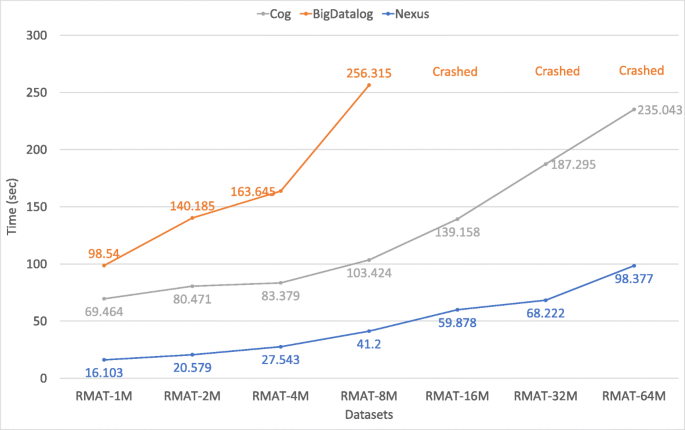
Performance comparison using the Reachability program on different graph sizes (for configuration 2)
Figure 11 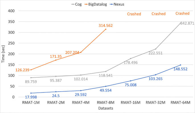
Performance comparison using the Reachability program on different graph sizes (for configuration 3)
Figure 12 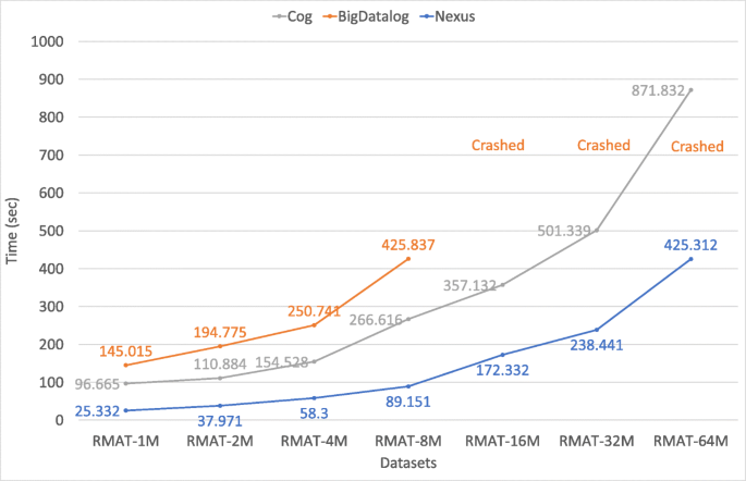
Performance comparison using the Reachability program on different graph sizes (for configuration 4)
We also observed that BigDatalog crashed due to running out of memory for all the datasets of sizes greater than RMAT-8M. Overall, Nexus is upto 3.9 × faster than Cog and 5.1 × faster than BigDatalog for RMAT dataset with configuration 1; upto 4.3 × faster than Cog and 6.8 × faster than BigDatalog for RMAT dataset with configuration 2; and upto 4.9 × faster than Cog and 7.0 × faster than BigDatalog for RMAT dataset with configuration 3; and upto 3.8 × faster than Cog and 5.7 × faster than BigDatalog for RMAT dataset with configuration 4.
Note that this difference in the execution time could get even larger if BigDatalog did not crash with larger datasets.


Evaluating Aggregate Programs
-
1.
Connected Components (CC): Figures 13, 14, 15, and 16 show the results of our experimental comparison for the CC program with RMAT datasets of varying sizes. The results show that the semi-naive evaluation using Flink’s delta iteration clearly offers significant advantage in all cases even for programs with recursive aggregates. Nexus performs 1.2 − 3 × faster than BigDatalog for configuration 1, 1.6 − 3.7 × faster for configuration 2, 2.2 − 4.5 × faster for configuration 3, and 1.6 − 2.2 × faster for configuration 4. BigDatalog could not complete for dataset sizes larger than RMAT-8M created using any of the given configurations. Note that the increase in time with the twofold increase in the dataset is between: 1.04 − 1.4 × for Nexus and 1.0 − 2.0 × for BigDatalog with configuration 1; 1.1 − 1.6 × for Nexus and 1.5 − 1.7 × for BigDatalog with configuration 2; 1.2 − 1.5 × for Nexus and 1.4 − 1.8 × for BigDatalog with configuration 3; and 1.2 − 1.4 × for Nexus and 1.1 − 1.7 × for BigDatalog with configuration 4.
-
2.
Single-Source Shortest Path (SSSP): Figures 17, 18, 19, and 20 show the result of our experimental comparison using the SSSP program with RMAT datasets of varying sizes and configurations (as provided in Section 7.1). For Nexus, the increase in the execution time is within 1.1 − 1.8 × for each twofold increase in the dataset size for configuration 1; 1.0 − 1.7 × for configuration 2; 1.1 − 1.8 × for configuration 3; and 1.0 − 1.6 × for configuration 4. For the datasets RMAT-1M to RMAT-16M, the increase in the execution time is insignificant for all the experiments. For BigDatalog, the variance in the result is surprisingly high for large datasets due to data spilling to disk (i.e., missing blocks in memory). BigDatalog could not finish for datasets larger than RMAT-8M. Yet, Nexus performs 2.7 − 4.7 × faster than BigDatalog for configuration1; 1.7 − 3.1 × faster for configuration2; 2.0 − 3.4 × faster for configuration3; and 1.7 − 2.7 × faster for configuration4 for the experiments that were completed.
-
3.
PageRank (PageRank): Figure 21 illustrates the result of our experimental comparison using the PageRank program (provided in Figure 16) with Arabic-2005 and UK-2005 real-world datasets. We compare the performance of Nexus with BigDatalog. We used 20 iterations for each case of our experiments. In our experiments, we show that Nexus performed slightly better than BigDatalog in all experiments. The reason for Nexus not achieving a significant performance advantage is that for each iteration, all tuples (after updating their ranks) are forwarded to the subsequent iteration until the specified iteration threshold is reached.

Performance comparison using the CC program (which includes aggregation) on RMAT graphs of varying sizes (for configuration 1)

Performance comparison using the CC program (which includes aggregation) on RMAT graphs of varying sizes (for configuration 2)

Performance comparison using the CC program (which includes aggregation) on RMAT graphs of varying sizes (for configuration 3)

Performance comparison using the CC program (which includes aggregation) on RMAT graphs of varying sizes (for configuration 4)

Performance comparison using the SSSP program (which includes aggregation) on RMAT graphs of varying sizes (for configuration 1)

Performance comparison using the SSSP program (which includes aggregation) on RMAT graphs of varying sizes (for configuration 2)

Performance comparison using the SSSP program (which includes aggregation) on RMAT graphs of varying sizes (for configuration 3)

Performance comparison using the SSSP program (which includes aggregation) on RMAT graphs of varying sizes (for configuration 4)

Performance comparison for the PageRank program
Experiments with Real-World Datasets
We also perform experiments using the Reachability, CC, and SSSP programs with the real-world graph datasets (shown in Table 3) for the batch case. Figure 22 shows the results of our experimental comparison. We observe that Nexus outperforms BigDatalog in all cases: for the Reachability program, Nexus performs 2.5 × and 3.4 × faster; for the CC program, 4.2 × and 3.1 × faster; and 3.8 × and 3.4 × faster for SSSP when using the LJ and Orkut datasets, respectively.

Performance comparison when using real-world datasets
Furthermore, we also perform experiments using the Reachability, CC, and SSSP programs with large-scale (i.e., upto billion edges) real-world graph datasets. Figure 23 shows the results of our experimental comparison. We show that Nexus outperforms BigDatalog by 3.4 − 3.9 × for the Reachability program, 3.3 − 4.1 × for the CC program, and 2.8 − 5.0 × for the SSSP when using the Arabic-2005, UK-2005, Twitter-2010, and SK-2005 datasets. BigDatalog suffers from scheduling overhead and slow data loading time.

Performance comparisons of Reachability, CC, and SSSP programs with large-scale real-world datasets
7.3 Scalability
We evaluate how our system’s execution time responds to: (i) increasing the number of nodes in the cluster (i.e., by scaling-out cluster size), and (ii) keeping the number of nodes the same but increasing the dataset sizes (i.e., by scaling-up the dataset size).
Scaling-out cluster size
In these set of experiments, we used the G10K graphs on a varying number of worker nodes (ranging between 1 and 24). We also used the TC and SG recursive programs for the batch processing case to measure speedup with the increase in the cluster size. Figures 24 and 25 shows the results of these experiments for TC and SG programs, respectively. We observe that the speedup with the increase in the workers from 1 to 24 for TC is 11 × and for SG is 23 ×.

Measuring speed-up achieved by scaling-out cluster size for TC program

Measuring speed-up achieved by scaling-out cluster size for SG program
Scaling-up dataset sizes
Here we kept the cluster size fixed (i.e., 24 workers) and used dataset of different sizes. We used Reachability program with RMAT graphs of increasing sizes (from 10m edges to 640m edges) to evaluate how well our system scales-up. Figure 26 shows the result of our scaling-up experiments. We observe a small increase in the time with the twofold increase in the dataset size. The increase in time is caused by the gradual increase in the output and intermediate tuple sizes with each doubling of the input dataset size.

Scaling-up on RMAT graph of increasing sizes using the Reachability program (streaming case)
8 Related work
Many works discuss efficient Datalog evaluation [5, 15, 34]. Here, we mostly focus on distributed systems.
Distributed Dataflow Systems
Apache Flink [1, 10] is a distributed dataflow system for large-scale data analytics. Flink supports cyclic dataflows, which we build on. Apache Spark [39] is also a scalable distributed dataflow system. However, in contrast to Flink, Spark does not allow for cyclic dataflow jobs, which means that a significant job launch overhead is introduced for iterative programs. Naiad [26] is another distributed dataflow system, and is based on the Timely Dataflow computation model. It supports cyclic dataflows, and therefore, it could be used for efficient Datalog execution, similarly to our Flink-based implementation. McSherry [25], Ryzhyk et al. [30], and Göbel et al. [17] go in this direction with a Rust reimplementation of the Timely Dataflow model. We chose Flink for our implementation because of its large user base, and also because we wanted a fair comparison against Cog, which is already implemented using Flink. Compiling to a different dataflow system could result in performance differences stemming from low-level implementation details of the dataflow systems (such as native code vs. Java), rather than on more important differences, such as removing the synchronization barrier between iterations, which is the main factor in our performance difference to Cog.
Pregel-like Graph Processing
Pregel [24] introduced the think-like-a-vertex programming model for scalable graph processing. This model is used in many large-scale graph processing systems, such as Giraph [41], GraphX [18], and Gelly [42]. In contrast to Datalog, the think-like-a-vertex programming model is a stateful computation model, whereas Datalog queries are more declarative. Note that Pregel-like systems often support the deactivation of vertices, which allows them to implement a form of incrementalization, similar to the incremental nature of semi-naive evaluation.
Datalog Evaluation in Distributed Systems.
There are several systems for executing Datalog programs on a cluster of machines. BigDatalog [33] implemented positive Datalog with recursion, non-monotonic aggregations, and aggregation in recursion with monotonic aggregates on Spark. In contrast to BigDatalog, Nexus supports non-monotonic aggregations in recursion. Furthermore, at the execution level, we differ by having asynchronous iterations, and by relying on cyclic dataflows. Cyclic dataflows are important for iterative computations, but BigDatalog has to rely on acyclic dataflows, as it uses Spark as an execution engine. BigDatalog uses a number of clever tricks to overcome some of the limitations of Spark due to acyclic dataflows. To avoid the job launching overhead, it added a specialized Spark stage (FixPointStage) for scheduler-aware recursion. Furthermore, reusing Spark tasks within a FixPointStage eliminates the cost of task scheduling and task creation; however, task reuse can only happen on so-called decomposable Datalog programs, and only when the joins can be implemented by broadcasting instead of repartitioning, which is not the case for large graphs. BigDatalog added specialized SetRDD and AggregateRDD to enable incremental updates to the solution set. BigDatalog also pays special attention to joins with loop-invariant inputs. It avoids repartitioning the static input of the join, as well as rebuilding the join’s hash table at every iteration. However, it does not ensure co-location of the join tasks with the corresponding cached build-side blocks, and thus cannot always avoid a network transfer of the build-side. (RaSQL [19] uses the same techniques plus operator code generation and operator fusion to implement recursive SQL with aggregations on Spark.)
When implementing Nexus, we did not need to perform any of the above optimizations of BigDatalog, as Flink has built-in support for efficient iterations with cyclic dataflow jobs. Having cyclic dataflow jobs means that all of the issues that BigDatalog’s optimizations are solving either do not even come up (per-iteration job-launching overhead and task-scheduling overhead), or already have simple solutions by keeping operator states across iterations (loop-invariant join inputs, incremental updates to the solution set). Thus, our view is that relying on Flink’s native iterations being implemented as a single, cyclic dataflow job is a more natural way to evaluate Datalog (or recursive SQL) efficiently.
Distributed SociaLite [32], is a system developed for social network analysis that implemented Datalog with recursive aggregate functions using a delta stepping method and gives the ability to programmers to specify data distribution. It uses message passing mechanism for communication among workers. We rely on SociaLite’s theoretical considerations for knowing when semi-naive evaluation can be used in the presence of recursive aggregations [31]. Note that Distributed SociaLite shows weaknesses in loading datasets (base relations) and poor shuffling performance on large datasets [33]. Myria [36] is a distributed execution engine that implemented Datalog with recursive monotonic aggregation function in a share-nothing engine and supports synchronous and asynchronous iterative models. Myria, however, suffers from shuffling overhead when running large datasets and becomes unstable (it often runs out of memory) [33].
Chothia et al. [12] focus on provenance tracking for arbitrary iterative dataflows, including Datalog queries. They rely on Timely Dataflow, while our system implementation is based on Flink.
GraphRex [40] is a recent distributed graph processing system with a Datalog-like interface. It focuses on making full use of the characteristics of modern data center networks, and thus achieves very high performance in such an environment. PowerLog [37] focuses on efficient asynchronous iteration in the presence of recursive aggregations, and has an MPI-based implementation. In contrast to Nexus, both GraphRex and PowerLog are standalone systems, i.e., they do not rely on an existing dataflow engine, such as Flink or Spark. Note that integration into an existing dataflow engine has the advantage that Datalog queries can be seamlessly integrated into larger data analytics programs written in a more general dataflow API.
9 Conclusion
We presented Nexus, a Datalog evaluation technique on top of Apache Flink. Nexus uses Flink’s delta iteration and asynchronous iterations for batch and streaming data, respectively. It provides a declarative, succinct interface to implement complex analytic tasks for both static and continuous data streams. Our experiments showed that our system provides superior performance compared to an acyclic data flow-based system. We also showed that with asynchronous iterations, we avoid barrier synchronization overhead, and programs run even faster than when only delta iteration is used.
Future Work
The current implementation for the streaming case considers incoming stream(s) of infinite data. However, users often need to apply Datalog rules on subsets of streams to limit memory usage. Therefore, introducing the notion of windowing is desired. User-defined aggregates functions can be implemented to allow users to perform custom aggregate operations. The mutual recursion case can also be implemented to benchmark how mutual recursion performs with distributed, cyclic dataflow compared to acyclic dataflow (such as Spark). Furthermore, implementing the linear algebra model on top of the relational algebra model in Nexus will enable users to perform machine learning and linear programming tasks declaratively using Datalog rules.
References
Alexandrov, A., Bergmann, R., Ewen, S., Freytag, J. C., Hueske, F., Heise, A., Kao, O., Leich, M., Leser, U., Markl, V., Naumann, F., Peters, M., Rheinländer, A., Sax, M. J., Schelter, S., Höger, M., Tzoumas, K., Warneke, D.: The Stratosphere platform for big data analytics. VLDB J. 23(6), 939–964 (2014)
Arni, F., Ong, K., Tsur, S., Wang, H., Zaniolo, C.: The deductive database system LDL++. Theory Pract. Log. Program. 3(1), 61–94 (2003)
Bancilhon, F.: Naive Evaluation of Recursively Defined Relations. In: On Knowledge Base Management Systems, pp. 165–178. Springer (1986)
Bancilhon, F.: Naive Evaluation of Recursively Defined Relations, pp. 165–178. Springer, Berlin (1986)
Bancilhon, F., Ramakrishnan, R.: An Amateur’s Introduction to Recursive Query Processing Strategies. In: Readings in Artificial Intelligence and Databases, pp. 376–430. Elsevier (1989)
Begoli, E., Camacho-rodríguez, J., Hyde, J., Mior, M.J., Lemire, D.: Apache Calcite: A foundational framework for optimized query processing over heterogeneous data sources. In: Proceedings of the 2018 International Conference on Management of Data, pp. 221–230 (2018)
Boldi, P., Rosa, M., Santini, M., Vigna, S.: Layered label propagation: a multiresolution coordinate-free ordering for compressing social networks. In: Srinivasan, S., Ramamritham, K., Kumar, A., Ravindra, M.P., Bertino, E., Kumar, R. (eds.) Proceedings of the 20th international conference on World Wide Web, pp 587–596. ACM Press (2011)
Boldi, P., Vigna, S.: The WebGraph Framework I: Compression Techniques. In: Proc. of the Thirteenth International World Wide Web Conference (WWW 2004), pp. 595–601. ACM Press, Manhattan (2004)
Brin, S., Page, L.: The anatomy of a large-scale hypertextual Web search engine. Comput. Netw. ISDN Syst. 30(1), 107–117. https://doi.org/10.1016/S0169-7552(98)00110-X. https://www.sciencedirect.com/science/article/pii/S016975529800110X. Proceedings of the Seventh International World Wide Web Conference (1998)
Carbone, P., Katsifodimos, A., Ewen, S., Markl, V., Haridi, S., Tzoumas, K.: Apache Flink: Stream and batch processing in a single engine. Bullet. IEEE Comput. Soc. Tech. Committee Data Eng. 36(4) (2015)
Ceri, S., Gottlob, G., Tanca, L.: What you always wanted to know about datalog (and never dared to ask). IEEE Trans. Knowl. data Eng. 1(1), 146–166 (1989)
Chothia, Z., Liagouris, J., McSherry, F., Roscoe, T.: Explaining Outputs in Modern Data Analytics. Technical report, ETH Zurich (2016)
Contreras-Rojas, B., Quiané-Ruiz, J. A., Kaoudi, Z., Thirumuruganathan, S.: Tagsniff: Simplified big data debugging for dataflow jobs. In: Proceedings of the ACM Symposium on Cloud Computing, SoCC ’19, pp. 453–464. Association for Computing Machinery, New York. https://doi.org/10.1145/3357223.3362738 (2019)
Ewen, S., Tzoumas, K., Kaufmann, M., Markl, V.: Spinning fast iterative data flows. Proc. VLDB Endow. 5(11), 1268–1279 (2012)
Fan, Z., Zhu, J., Zhang, Z., Albarghouthi, A., Koutris, P., Patel, J.: Scaling-up in-memory Datalog processing: observations and techniques. arXiv:1812.03975 (2018)
Gévay, G. E., Rabl, T., Breß, S., Madai-Tahy, L., Markl, V.: Labyrinth: Compiling imperative control flow to parallel dataflows. arXiv:1809.06845 (2018)
Göbel, N., Bach, D., McSherry, F., Sandstede, M.: Declarative dataflow. https://github.com/comnik/declarative-dataflow. [Online; accessed 20-July-2020] (2019)
Gonzalez, J. E., Xin, R. S., Dave, A., Crankshaw, D., Franklin, M. J., Stoica, I.: GraphX: Graph Processing in a Distributed Dataflow Framework. In: 11Th USENIX Symposium on Operating Systems Design and Implementation OSDI 14), pp. 599–613 (2014)
Gu, J., Watanabe, Y. H., Mazza, W. A., Shkapsky, A., Yang, M., Ding, L., Zaniolo, C.: RaSQL: Greater power and performance for big data analytics with recursive-aggregate-SQL on Spark. In: Proceedings of the 2019 International Conference on Management of Data, pp. 467–484 (2019)
Imran, M., Gévay, G.E., Markl, V.: Distributed graph analytics with Datalog queries in Flink. LSGDA 2020 - International Workshop on Large Scale Graph Data Analytics. http://www.redaktion.tu-berlin.de/fileadmin/fg131/Publikation/Papers/datalog-to-flink_2020.pdf (2020)
Imran, M., Gévay, G. E., Markl, V.: Distributed Graph Analytics with Datalog Queries in Flink. In: Qin, L., Zhang, W., Zhang, Y., Peng, Y., Kato, H., Wang, W., Xiao, C. (eds.) Software Foundations for Data Interoperability and Large Scale Graph Data Analytics, pp 70–83. Springer International Publishing, Cham (2020)
Kejariwal, A., Kulkarni, S., Ramasamy, K.: Real time analytics: Algorithms and systems. Proc. VLDB Endow. 8(12), 2040–2041 (2015). https://doi.org/10.14778/2824032.2824132
Lloyd, J. W.: Foundations of logic programming. Springer, Berlin (1984)
Malewicz, G., Austern, M. H., Bik, A. J., Dehnert, J. C., Horn, I., Leiser, N., Czajkowski, G.: Pregel: a system for large-scale graph processing. In: Proceedings of the 2010 ACM SIGMOD International Conference on Management of data, pp. 135–146 (2010)
McSherry, F.: Differential datalog. https://github.com/frankmcsherry/blog/blob/master/posts/2016-06-21.md [Online; Accessed 19 2021]
Murray, D. G., McSherry, F., Isaacs, R., Isard, M., Barham, P., Abadi, M.: Naiad: a timely dataflow system. In: Proceedings of the Twenty-Fourth ACM Symposium on Operating Systems Principles, pp. 439–455 (2013)
Palla, G., Derényi, I., Farkas, I., Vicsek, T.: Uncovering the overlapping community structure of complex networks in nature and society. Nature 435(7043), 814–818 (2005)
Parr, T., Harwell, S., Fisher, K.: Adaptive LL(*) parsing: The power of dynamic analysis. In: Proceedings of the 2014 ACM International Conference on Object Oriented Programming Systems Languages & Applications, OOPSLA ’14, pp. 579–598. Association for Computing Machinery, New York. https://doi.org/10.1145/2660193.2660202 (2014)
Raymond, J.W., Gardiner, E.J., Willett, P.: Rascal: Calculation of graph similarity using maximum common edge subgraphs. Comput. J. 45(6), 631–644 (2002). https://doi.org/10.1093/comjnl/45.6.631
Ryzhyk, L., Budiu, M.: Differential Datalog. In: Datalog 2.0 – 3Rd International Workshop on the Resurgence of Datalog in Academia and Industry. CEUR-WS (2019)
Seo, J., Guo, S., Lam, M. S.: Socialite: Datalog Extensions for Efficient Social Network Analysis. In: 2013 IEEE 29Th International Conference on Data Engineering (ICDE), pp. 278–289. IEEE (2013)
Seo, J., Park, J., Shin, J., Lam, M. S.: Distributed SociaLite: A Datalog-based language for large-scale graph analysis. Proc. VLDB Endowment 6(14), 1906–1917 (2013)
Shkapsky, A., Yang, M., Interlandi, M., Chiu, H., Condie, T., Zaniolo, C.: Big Data Analytics with Datalog Queries on Spark. In: SIGMOD, pp. 1135–1149 (2016)
Subotić, P., Jordan, H., Chang, L., Fekete, A., Scholz, B.: Automatic index selection for large-scale Datalog computation. Proc. VLDB Endowment 12(2), 141–153 (2018)
Vieille, L.: A Database-Complete Proof Procedure Based on Sld-Resolution. In: ICLP (1987)
Wang, J., Balazinska, M., Halperin, D.: Asynchronous and fault-tolerant recursive Datalog evaluation in shared-nothing engines. Proc. VLDB Endowment 8 (12), 1542–1553 (2015)
Wang, Q., Zhang, Y., Wang, H., Geng, L., Lee, R., Zhang, X., Yu, G.: Automating incremental and asynchronous evaluation for recursive aggregate data processing. In: Proceedings of the 2020 ACM SIGMOD International Conference on Management of Data, pp. 2439–2454 (2020)
Yook, S. H., Oltvai, Z. N., Barabási, A. L.: Functional and topological characterization of protein interaction networks. Proteomics 4(4), 928–942 (2004)
Zaharia, M., Chowdhury, M., Franklin, M. J., Shenker, S., Stoica, I., et al.: Spark: Cluster computing with working sets. HotCloud 10(10-10), 95 (2010)
Zhang, Q., Acharya, A., Chen, H., Arora, S., Chen, A., Liu, V., Loo, B. T.: Optimizing declarative graph queries at large scale. In: Proceedings of the 2019 International Conference on Management of Data, pp. 1411–1428 (2019)
Apache Giraph. http://giraph.apache.org/. [Online; Accessed 12 Apr. 2020]
Gelly: Flink Graph API. https://ci.apache.org/projects/flink/flink-docs-stable/dev/libs/gelly/. [Online; Accessed 12 Apr. 2020]
GTGraph. http://www.cse.psu.edu/~kxm85/software/GTgraph/. [Online; Accessed 12 Apr. 2020]
Livejournal dataset. http://snap.stanford.edu/data/com-LiveJournal.html. [Online; Accessed 2 Mar. 2021]
Orkut dataset. http://snap.stanford.edu/data/com-Orkut.html. [Online; Accessed 12 Mar. 2021]
Funding
Open Access funding enabled and organized by Projekt DEAL. This work was funded by the German Ministry for Education and Research as BIFOLD (01IS18025A and 01IS18037A) and the German Research Foundation (Project-ID 414984028 - SFB 1404 FONDA).
Author information
Authors and Affiliations
Corresponding author
Additional information
Publisher’s note
Springer Nature remains neutral with regard to jurisdictional claims in published maps and institutional affiliations.
This article belongs to the Topical Collection: Special Issue on Large Scale Graph Data Analytics
Guest Editors: Xuemin Lin, Lu Qin, Wenjie Zhang, and Ying Zhang
Rights and permissions
Open Access This article is licensed under a Creative Commons Attribution 4.0 International License, which permits use, sharing, adaptation, distribution and reproduction in any medium or format, as long as you give appropriate credit to the original author(s) and the source, provide a link to the Creative Commons licence, and indicate if changes were made. The images or other third party material in this article are included in the article's Creative Commons licence, unless indicated otherwise in a credit line to the material. If material is not included in the article's Creative Commons licence and your intended use is not permitted by statutory regulation or exceeds the permitted use, you will need to obtain permission directly from the copyright holder. To view a copy of this licence, visit http://creativecommons.org/licenses/by/4.0/.
About this article

Cite this article
Imran, M., Gévay, G.E., Quiané-Ruiz, JA. et al. Fast datalog evaluation for batch and stream graph processing. World Wide Web 25, 971–1003 (2022). https://doi.org/10.1007/s11280-021-00960-w
Received:
Revised:
Accepted:
Published:
Issue Date:
DOI: https://doi.org/10.1007/s11280-021-00960-w