Sum-rate maximization for a distributed space-time block code-aided cooperative NOMA with energy harvesting

Abstract

In this paper, we exploit the spatial and transmission diversities in cooperative non-orthogonal multiple access (C-NOMA) networks to improve the system sum-rate. To achieve this, we propose a user-pairing scheme where near-field user pairs serve as relays for user pairs in the far-field region. Based on this pairing scheme, we incorporate a space-time block code transmission technique at the near-field user pairs to maximize the transmission diversity in the cooperative phase. Moreover, we consider a non-linear energy harvesting model at the near-field user pair to alleviate the problem of energy consumption during the cooperative transmission phase. Further to this, we formulate a sum-rate maximization problem that is addressed from the viewpoint of joint power allocation factor and power splitting ratio optimization. We develop a low-computational iterative algorithm based on the concepts of the Stackelberg game and the Nash bargaining solution. We benchmark our findings with different scenarios, such as energy harvesting C-NOMA with a fixed power allocation factor and power splitting ratio, energy harvesting C-NOMA without STBC, non-cooperative NOMA, and orthogonal multiple access. The results obtained via simulations outperform the benchmark schemes.

1 Introduction

The field of wireless communication networks continues to experience paradigm shifts, manifesting through the evolution of different generations of mobile communication networks. This can be attributed to the widespread applications of wireless technologies in various fields, coupled with the exponential growth of wireless-enabled devices. According to Cisco’s projection, the number of wireless-enabled devices is envisioned to exceed 40 billion by 2023 [1]. These devices are expected to be smartly connected via the internet while executing various data-intensive services. Interestingly, the fifth generation (5G) and beyond technologies are being deployed to satisfy the quality of service (QoS) demands of these devices [2].

One of these key technologies belongs to the category of next-generation multiple access technologies, namely power-domain non-orthogonal multiple access (PD-NOMA) [3]. By assigning different transmission power levels to users, the PD-NOMA serves multiple users over the same time and frequency resources [4]. Due to this attribute, PD-NOMA outperforms the conventional orthogonal multiple access (OMA) techniques in terms of user fairness, spectral efficiency, and low-latency transmission [5].

To enhance the performance of PD-NOMA, the incorporation of cooperative communication in this technology, dubbed cooperative NOMA (C-NOMA) has been proposed and proven to be efficient for improving spatial diversity gain [6]. C-NOMA is achieved by enabling near-field devices to serve as relays for far-field or cell-edge devices [7, 8]. Moreover, these relays adopt well-established relaying protocols such as amplify-and-forward (AF) or decode-and-forward (DF) in the cooperative phase of the transmission [9].

Furthermore, the transmit diversity in the cooperative phase can be exploited for improved end-to-end transmission by employing the concept of space-time block coding (STBC), discovered by Alamouti [10]. In this approach, multiple relays operate together such that two signals are simultaneously transmitted from each relay to the destination receiver at a given symbol period [11]. The destination receiver achieves full transmit diversity gain by combining all the received signals in order to decode its messages using maximum ratio combining (MRC) and the maximum likelihood decision rule.

However, an increase in energy consumption of the relays during the cooperative STBC phase is inevitable since the energy required for computation and transmission is drawn from their batteries, which have limited storage capacity [12,13,14,15,16,17]. To address this challenge, a radio frequency (RF) energy harvesting technique known as simultaneous wireless information and power transfer (SWIPT) constitutes one of the viable solutions [18,19,20]. SWIPT technique uses power splitting (PS) or time switching (TS) protocols to partition the received signals at the relays for concurrent information decoding (ID) and energy harvesting (EH) [21]. Nonetheless, developing a realistic unification system that combines PD-NOMA, cooperative STBC transmission and SWIPT, without violating QoS requirements poses a major challenge in the open literature.

1.1 Related works

In the open literature, several studies have been devoted to evaluating and optimizing the performance of SWIPT-aided C-NOMA networks. In [22], the outage probability (OP) expression for the cell-edge and cell-center users are derived in closed-form. Furthermore, the sum-throughput maximization problem for the system is solved by optimizing the transmission time fraction and PS ratio. In [23], the impact of PS and TS protocols on the OP and system throughput is examined. Results obtained show that the TS has better performance. In another related work but more complex scenario [24], the end-to-end OP is evaluated in closed-form for a downlink and uplink transmission under a four-hop transmission condition and imperfect successive interference cancellation (SIC). Furthermore, the bit error rate (BER) analysis and impact of residual hardware impairment are conducted in [25, 26] and [27], respectively. In [25], a hybrid PS-TS protocol is developed to improve the end-to-end BER and OP of the system. In [26], the impact of inter-user interference (ICI) and imperfect SIC on BER is investigated under TS protocol and imperfect CSI conditions. Findings show that ICI leads to the deterioration of the performance of SIC and consequently creates an error floor at a high signal-to-noise ratio (SNR). In [27], the effect of hardware impairment on the OP of the system is evaluated under time switching and power splitting protocols. In [28], the concept of data buffering at the EH relay is investigated. In the study, the data stored in the relay buffer is only transmitted to the destination on a link with strong channel gain. In [29], the use of an acknowledgment signal is proposed to determine whether a relay or direct link should be used for transmission to the destination receiver. The goal is to maximize the throughput of the system based on the Markov decision process.

From the viewpoint of multiple near-field users (NUEs) and far-field users (FUE), the authors of [30], investigate the OP and delay-limited throughput of the system. Though the study highlights the advantages of user pairing, details on this are not captured. This limitation is addressed in [31], where user pairing and resource allocation problems for sum-rate maximization are investigated. In [32], the effect of a partial relay selection based on the source-relay channel gain is investigated. The goal is to analyze the undecodable probability of the received symbol at the relay and destination, and the ergodic capacity of the system under perfect and imperfect SIC. However, a realistic system model that captures the random distribution of users is not considered. This limitation forms the basis of the studies presented in [33,34,35] where stochastic geometry is employed for system modeling. In [33], the nearest near and nearest far (NNNF), the nearest near and farthest far (NNFF), and random near and random far (RNRF) user pairing based on user location information is proposed. Though the NNNF has the best overall performance in terms of OP, throughput, diversity order and multiplexing, the RNRF has the best performance in terms of user fairness. In [34] the OP and throughput are derived and solved in closed-form. Moreover, the Repulsive point process, aided by carrier sensing is proposed for the accurate modelling of small cells to create an interference restriction region. The study is further extended in [35] where imperfect CSI condition and EH from interference signals from adjacent BS are considered in the system design.

While some studies have focused on the physical layer security design of the system [36,37,38], others have investigated the system performance based on the integration of cutting-edge technologies such as a dedicated power beacon for EH [39, 40], full-duplex relaying, [41,42,43] multiple-input-multiple-output (MIMO) [44, 45], and reconfigurable intelligent surface [46]. However, few papers have considered the integration of the STBC technique to enhance the end-to-end achievable rate. These limitations form the basis of the studies presented in [47,48,49,50,51]. In [47], a dual relay selection algorithm is proposed, based on which the closed-form OP of the system is derived. However, the relay selection process may be invalid in a distributed scenario where multiple STBC groups are desired. This limitation is addressed in [48], where the users are first partitioned into even and odd users before user pairing. Furthermore, the effect of the timing offset and imperfect SIC during the STBC transmission phase is also investigated. Findings from analytical results show that increasing the timing offset factor decreases the average system SNR. However, EH is not considered in [47, 48]. In [49], EH is considered in the system design, where the performance of the system throughput under three relay selection schemes is investigated. Based on the minimum and largest sum of signal power fading, max-min and max-sum relay selection schemes are proposed, respectively, in addition to a random selection scheme. The max-sum approach has the best overall performance. In [50], the study is extended to capture the impact of the channel estimation error of the system OP, sum-throughput and energy efficiency. Nevertheless, the non-linear EH model and multiple relays are not considered in [49] and [50]. These limitations have been addressed in our previous work [51] where we employ a dual relay selection scheme and non-linear EH model. In the study [51], we develop a near-optimal solution that jointly optimizes the power allocation factor and PS ratio by employing the principle of Nash bargaining solution. The goal is to maximize the achievable rate of the users. Our approach outperforms the benchmark solutions based on conventional NOMA and OMA.

1.2 Motivation and contributions

Over the years, there have been relentless efforts from academia and industry towards developing 5 G and B5G technologies to support an easy transition from the age of internet-of-things to the era of internet-of-everything (IoE) [52]. The adoption of the C-NOMA technique is deemed suitable to support network scalability and user fairness in IoE networks. Moreover, the C-NOMA technique is cost-effective since it can be established between the existing nodes in a network without the requirement of additional network infrastructure. However, due to the dynamic nature of the radio environment, deep fading caused by obstacles and pathloss is inevitable for weak or cell-edge users. Also, these devices are battery-constrained; hence, sustaining their lifetime remains a major challenge.

Interestingly, an STBC-based C-NOMA technique with energy harvesting capacity has been proposed to address this challenge. Nonetheless, there remain open issues yet to be addressed. Based on the studies in this direction [47,48,49,50,51], the sustainability of the network proposed in [47, 48] remains a major issue due to their non-consideration of EH. Though the studies presented in [49, 50] consider a linear EH model, the STBC transmission is only implemented between the source and a single relay, without exploiting the additional spatial and transmission diversities of the users in the network. These limitations are addressed in our previous study [51], where a dual relay selection and non-linear EH are proposed for STBC transmission in the cooperative phase. Moreover, a near-optimal solution based on the Nash bargaining solution is developed to deal with the problem of complex analytical solutions proposed in previous studies. In addition, the proposed system model is designed for a single STBC group where only one user in the far-field region is served. However, this approach may not support scalability in massive user deployment scenarios. Therefore, we aim to bridge the aforementioned gaps in this present study. The contributions of this article are presented in the following:

• We incorporate a robust user pairing scheme in the system model capable of supporting the establishment of multiple STBC groups under even and odd numbers of user deployment scenarios. We employ a piecewise-based non-linear EH model at the selected relays as a means of compensating for energy consumed in the cooperative phase.

• Based on the STBC transmission scheme, we formulate the expression for the sum-rate maximization problem in the system, which is constrained by the individual utility. We later transform the sum-rate maximization into a buyer-seller bargaining problem based on the Stackelberg game and Nash bargaining solution.

• We solve the optimization problem by developing an iterative algorithm that jointly maximizes the power allocation factor and power splitting ratio. Furthermore, the energy efficiency of the system is evaluated. Finally, we show via simulations that our proposed solution outperforms the baseline schemes.

The rest of the article is structured as follows: In Sect. 2, the system model is developed. The sum-rate maximization problem is formulated in Sect. 3. The proposed joint iterative algorithm solution is presented in Sect. 4. Simulation results and discussion of our findings are presented in Sect. 5. Finally, conclusions are drawn in Sect. 6.

2 System model

We consider a typical downlink of a cooperative mobile network, as illustrated in Fig. 1. The devices in the considered network can be deployed randomly or they can be placed at fixed random locations within the coverage area of a serving base station, also known as the source. In this manuscript, we consider the latter scenario. The illustrated network is assumed to be in a large-scale indoor environment such as a shopping mall, airport, train station, etc., where Pico or Femto BS are usually deployed.

Fig. 1

An illustration of the downlink model of the proposed cooperative mobile communication network

The source and the users are equipped with a single antenna. Depending on their channel gains from the source, each user is categorized as a near-field user (NUE) or a far-field user (FUE), unlike our previous work [51] where only one FUE was considered. This is to support network scalability because, in a more realistic network, there is a high possibility of the existence of multiple cell-edge users, which are also regarded as FUEs. Furthermore, we assume there is no direct link between the source and FUEs due to the presence of obstacles or deep fading caused by distance-related pathloss. Consequently, the NUEs are expected to establish cooperative communication by serving as relays for the FUEs. Moreover, we limit the number of FUEs that can be associated with a particular NUE to two to avoid overloading the NUEs acting as relays. Also, we constrain the number of NUEs that can be selected as relays to two to strike a balance between spectral efficiency and computational complexities [47], that may be associated with the proposed design.

In this study, we take into account the coverage scenarios where even and odd numbers of users are deployed. This is pertinent to support a realistic network design, in which the number of users in a network can either be even or odd. To compute the channel gains, it is assumed that the NUEs and FUEs share local information that is accessible by the source via the NUEs. After sorting the channel gains of all users, denoted by $U_k$, in descending order, their indexes are rearranged in ascending order to have $k \in \{1, 2, 3,\ldots , K\}$. If the number of sorted users is even, two sets of users, $U_{k_1},~ k_1 \in \{1, 2, \ldots , \frac{K}{2}-1,\frac{K}{2}\}$ which can be regarded as a set of NUE and $U_{k_2}, ~k_2 \in \{\frac{K}{2}+1, \frac{K}{2}+2, \ldots , K-1, K\}$ which can be regarded as a set of FUEs, are established, respectively. To perform user pairing, two instances are further considered, i.e., when the numbers of users in $U_{k_1}$ and $U_{k_2}$ are both even and odd. In the former case, we exploit the nearest near users and farthest far user (NNFF) selection strategy, where users 1 and 2 from $U_{k_1}$ are selected and paired with the last two users $K-1$ and K from $U_{k_2}$. A similar approach is adopted in the latter case, except that the remaining $\frac{K}{2}$ and $\frac{K}{2} + 1$ form a single user pair $k_3$.

Considering the case where the number of $U_k$ users is odd, three sets of users are initiated. Here, we have $U_{k_1},~ U_{k_2}$ and $U_{k_3}$ for $k_1 \in \{1, 2, \ldots , \frac{K-2}{2},\frac{K-1}{2}\}$, $k_2 \in \{\frac{K+2}{2}, \frac{K+3}{2}, \ldots , K-1, K\}$ and $k_3 \in \{\frac{K+1}{2}\}$, respectively. Users in $U_{k_1}$ and $U_{k_2}$ are considered for user pairing. The pairing scheme adopted in the even case is also applicable here. However, the set $U_{k_3}$ contains only the middle user, i.e., $k \in \{\frac{K+1}{2}\}$, hence, it is not considered in the pairing process. Note that in our algorithm, we denote $s_i$ as the pairs of i-th user in each STBC group. The proposed user pairing algorithm is present in Algorithm 1.

Algorithm 1

User Pairing Algorithm

In Algorithm 1, the input is initialized by the number of UEs deployed $U_k$ and their corresponding channel coefficients $h_k$. The expected output is the number of realizable NUE and FUE user pairs. In line 1, deployed UEs are sorted in descending order of their channel gains. In line 2, the scenario where the number of deployed UEs is even is executed. Line 3 validates that UEs are deployed within the network coverage. In line 4, the NUE and FUE sets are initialized for an even number of users after partitioning. The initialized FUE and NUE sets are populated in lines 5 and 6, respectively. In lines 7 and 8, the STBC groups are initialized. In line 9, the condition that an odd number of users exist after partitioning is considered. In line 10, the NUE and FUE sets are populated following the same steps in lines 4 to 7. Moreover, a third set is initialized in line 11 for the remaining UEs in the middle of the partition. In lines 12 and 13, the even and odd conditions for UE entries in the initialized set of the first case in line 2 are terminated. In line 14, the scenario where the number of deployed UEs is odd is executed. Line 15 validates that UEs are deployed within the network coverage. The initialized FUE and NUE in these sets are populated in lines 16 and 17, respectively, while the remaining UE in the middle partition is assigned to an initialized third set in line 18. In line 19, the STBC groups are initialized. Lines 20 and 21 represent the scenario where only one group and more than one STBC group are established, respectively. Line 22 ends the program execution of the second case, initiated in line 14.

Once the STBC groups are established, the source transmits a superimposed message to the NUEs. In this study, we consider the case where $K = 4$. Consequently, the NUEs in the STBC group are $U_1$ and $U_2$, and FUEs are $U_3$ and $U_4$ as depicted in Fig. 2.

Fig. 2

STBC transmission

Our proposed solution can be generalized for multiple m-th STBC groups.

2.1 Direct phase

Since the direct path does not exist between the source and the FUEs, the received signal in the direct phase by the NUEs can be written as

$$\begin{aligned} y_{(k)}^{(1)} =\sqrt{(1-\rho _{k})P_0}h_ {k}\Biggl (\sum _{k=1}^{2}\sqrt{\alpha _{k}}x_{k} + \sqrt{\alpha _{3}}x_3 + \sqrt{\alpha _{4}}x_4\Biggr ) + z_k, \end{aligned}$$

(1)

where $P_0$ is the power budget of the STBC group, $1-\rho _k$ represents the fraction of the received signal needed for ID, the power splitting ratio is represented by $\rho _{k}$ and the additive white Gaussian noise (AWGN) is represented by $z_{k} \sim \mathcal{C}\mathcal{N}(0,N_0)$.

For $U_{1}$ to decode its message, it first detects and subtracts the message of other users using successive interference cancellation (SIC). Thus, the expressions for the received SINR by $U_{1}$ to detect the messages of $U_{4}$, $U_{3}$ and $U_{2}$ are given in (2), (3), and (4) respectively.

$$\begin{aligned} \gamma _{{1},x_{4}}^{(1)} = \frac{(1-\rho _{1})|{h}_{1}|^{2}\alpha _{4}\beta _0}{(1-\rho _{1})|{h}_{1}|^{2}\sum _{k=1}^{3}\alpha _{k}\beta _0 + 1}, \end{aligned}$$

(2)

$$\begin{aligned} \gamma _{{1},x_{3}}^{(1)} = \frac{(1-\rho _{1})|{h}_{1}|^{2}\alpha _{3}\beta _0}{(1-\rho _{1})|{h}_{1}|^{2}\sum _{k=1}^{2}\alpha _{k}\beta _0 + 1}, \end{aligned}$$

(3)

$$\begin{aligned} \gamma _{{1},x_{2}}^{(1)} = \frac{(1-\rho _{1})|{h}_{1}|^{2}\alpha _{2}\beta _0}{(1-\rho _{1})|{h}_{1}|^{2}\alpha _{1}\beta _0 + 1}. \end{aligned}$$

(4)

After subtracting $x_{4}$, $x_{3}$ and $x_{2}$ from $y_{(k)}^{(1)}$, the SNR of $U_1$ to detect its signal can be written as

$$\begin{aligned} \gamma _{{1},x_{1}}^{(1)} = (1-\rho _{1})|{h}_{1}|^{2}\alpha _{1}\beta _0. \end{aligned}$$

(5)

In the case of $U_2$ the received SINR to detect the message $x_4$, $x_3$, and $x_1$ is given in (6), (7), and (8), respectively

$$\begin{aligned} \gamma _{{2},x_{4}}^{(1)} = \frac{(1-\rho _{2})|{h}_{2}|^{2}\alpha _{4}\beta _0}{(1-\rho _{2})|{h}_{2}|^{2}\sum _{k=1}^{3}\alpha _{k}\beta _0 + 1}, \end{aligned}$$

(6)

$$\begin{aligned} \gamma _{{2},x_{3}}^{(1)} = \frac{(1-\rho _{2})|{h}_{2}|^{2}\alpha _{3}\beta _0}{(1-\rho _{2})|{h}_{2}|^{2}\sum _{k=1}^{2}\alpha _{k}\beta _0 + 1}, \end{aligned}$$

(7)

$$\begin{aligned} \gamma _{{2},x_{1}}^{(1)} = (1-\rho _{2})|{h}_{2}|^{2}\alpha _{1}\beta _0. \end{aligned}$$

(8)

The SNR of $U_2$ to decode its message after subtracting $x_4$, $x_3$, and $x_1$ can be written as

$$\begin{aligned} \gamma _{{2},x_{2}}^{(1)} = \frac{(1-\rho _{2})|{h}_{2}|^{2}\alpha _{2}\beta _0}{(1-\rho _{2})|{h}_{2}|^{2}\alpha _{1}\beta _0 + 1}. \end{aligned}$$

(9)

Furthermore, we adopt a piecewise non-linear saturation EH model [53], which can be given as

$$\begin{aligned} \tilde{P}_{k} = {\left\{ \begin{array}{ll} 0, &{} \check{P}_0 < P_{h_{min}},\\ P_{k} = \eta _{k} \check{P}_0, &{} P_{h_{min}} \le \check{P}_0 \le P_{h_{max}},\\ \eta _k P_{h_{max}} &{} \check{P}_0 > P_{h_{max}}. \end{array}\right. } \end{aligned}$$

(10)

We can reformulate (10) as

$$\begin{aligned} \tilde{P}_{k} = {\left\{ \begin{array}{ll} 0, &{} \check{P}_0 < \frac{P_{h_{min}}}{\rho |{h}_{nk}|^{2}},\\ \eta _{k}\rho _{k}P_0|{h}_{k}|^{2}, &{} \frac{P_{h_{min}}}{\rho |{h}_{k}|^{2}} \le \check{P}_0 \le \frac{P_{h_{max}}}{\rho |{h}_{k}|^{2}},\\ \eta _{k} P_{h_{max}} &{} \check{P}_0 > \frac{P_{h_{max}}}{\rho |{h}_{k}|^{2}}. \end{array}\right. } \end{aligned}$$

(11)

In (11), $P_{h_{min}}$ and $P_{h_{max}}$ represent the minimum and maximum harvested power thresholds, respectively and $\eta _k$ is energy conversion efficiency. The conditions $\check{P}_0 < \frac{P_{h_{min}}}{\rho |{h}_{nk}|^{2}}$, $\frac{P_{h_{min}}}{\rho |{h}_{k}|^{2}} \le \check{P}_0 \le \frac{P_{h_{max}}}{\rho |{h}_{k}|^{2}}$, and $\check{P}_0 > \frac{P_{h_{max}}}{\rho |{h}_{k}|^{2}}$, represent the off, linear and saturation behaviour of the EH circuit, respectively.

2.2 Cooperative phase

The NUE pair $U_1$ and $U_2$ use the AF protocol to forward the information of FUE pair $U_3$ and $U_4$. However, if a user in the NUE pair is unable to successfully detect the message of users in the FUE pair, then the NUE pair does not participate in STBC cooperative transmission. Note that for the NUE pair to detect the message of other users successfully, they must satisfy the minimum rate threshold, i.e., $R_{k} \ge R_{min}$ and harvested power threshold i.e., $\tilde{P}_{k} \ge P_{h_{min}}$ thresholds. Therefore, from (5), and (9), the achievable rate of $U_1$ and $U_2$ can be given in (12) and (13), respectively.

$$\begin{aligned} R_{1} = \log _2(1 + (1-\rho _{1})|{h}_{1}|^{2}\alpha _{1}\beta _0), \end{aligned}$$

(12)

$$\begin{aligned} R_{2} = \log _2\Biggl (1 + \frac{(1-\rho _{2})|{h}_{2}|^{2}\alpha _{2}\beta _0}{(1-\rho _{2})|{h}_{2}|^{2}\alpha _{1}\beta _0 + 1}\Biggr ). \end{aligned}$$

(13)

In order to satisfy the case $R_{k} \ge R_{min}$, the expression in (12) and (13) can be further expressed as

$$\begin{aligned} (1-\rho _{1})|{h}_{1}|^{2}\alpha _{1}\beta _0 \ge 2^{R_{min}} - 1, \end{aligned}$$

(14)

and,

$$\begin{aligned} \frac{(1-\rho _{2})|{h}_{2}|^{2}\alpha _{2}\beta _0}{(1-\rho _{2})|{h}_{2}|^{2}\alpha _{1}\beta _0 + 1} \ge 2^{R_{min}} - 1, \end{aligned}$$

(15)

respectively. If the expressions in (14) and (15) are satisfied, then the received signal by $U_3$ and $U_{4}$ from $U_1$ and $U_2$ can be written as

$$\begin{aligned} y_{3,k} = \Gamma _{k}g_{k}y_{k}^{(1)} + z_{3}, \quad k \in \{1,2\}, \end{aligned}$$

(16)

and,

$$\begin{aligned} y_{4,k} = \Gamma _{k}g'_{k}y_{k}^{(1)} + z_{4}, \quad k \in \{1,2\}, \end{aligned}$$

(17)

respectively.

The parameter $g_{k}$ is the channel coefficients of $U_1$ and $U_2$ links serving $U_3$, $g'_{k}$ is the channel coefficients of $U_1$ and $U_2$ links serving $U_4$, $z_{3}$ and $z_{4}$ $\sim \mathcal{C}\mathcal{N}(0, N_0)$ represents the complex AWGN at their receivers respectively, and $\Gamma _{k}$ is the amplification coefficient which is given as [54].

$$\begin{aligned} \Gamma _{k} = \sqrt{\frac{\beta _{k}}{\beta _0\mathbb {E}|{\hat{g}}_{k}|^{2} + 1}}, \end{aligned}$$

(18)

where $\hat{g} \in \{g_k, g'_k\}$ represent the channel coefficients when either $U_3$ or $U_4$, is considered, $\beta _{k} = \frac{\tilde{P}_{k}}{N_0}$. Substituting (1) and (18) in (16) and (17) we have

$$\begin{aligned} y_{3,k} = g_{k}\Gamma _{k}\Biggl (\sqrt{(1-\rho _{k})P_0}h_ {k}\Biggl (\sum _{k=1}^{2}\sqrt{\alpha _{k}}x_{k} + \sqrt{\alpha _{3}}x_3 + \sqrt{\alpha _{4}}x_4\Biggr ) + z_k \Biggr )+ z_{3} \end{aligned},$$

(19)

$$\begin{aligned} y_{4,k} = g'_{k}\Gamma _{k}\Biggl (\sqrt{(1-\rho _{k})P_0}h_ {k}\Biggl (\sum _{k=1}^{2}\sqrt{\alpha _{k}}x_{k} + \sqrt{\alpha _{3}}x_3 + \sqrt{\alpha _{4}}x_4\Biggr ) + z_k \Biggr )+ z_{4}. \end{aligned}$$

(20)

The received SINR by a particular $U_{3}$ and $U_4$ form any pair of NUE to decode their messages, be written as

$$\begin{aligned} \gamma _{3,k}^{(2)} = \frac{\Gamma _{k}^2(1-\rho _k)|{g}_{k}|^{2}|{h}_{k}|^{2}\alpha _{3}\beta _{0}}{\Gamma _{k}(1-\rho _k)|{g}_{k}|^{2}|{h}_{k}|^{2}\alpha _{3}\beta _{0}(\sum _{k=1}^{2}+\alpha _4) + \Gamma _{k}^2|{g}_{k}|^{2} + 1}. \end{aligned}$$

(21)

Take $\Phi _{k} = \frac{1}{\Gamma _{{k}}^2|{g}_{k}|^{2}}$, then Eq. (21) can be simplified as

$$\begin{aligned} \gamma _{3,k}^{(2)} = \frac{(1-\rho _k)|{g}_{k}|^{2}|{h}_{k}|^{2}\alpha _{3}\beta _{0}}{(1-\rho _k)|{h}_{k}|^{2}\alpha _{3}\beta _{0}(\sum _{k=1}^{2}+\alpha _4) + 1 + \Phi _{k} }. \end{aligned}$$

(22)

At $U_4$, the received SINR to decode its message can be given as

$$\begin{aligned} \gamma _{4,k}^{(2)} = \frac{(1-\rho _k)|{g'}_{k}|^{2}|{h}_{k}|^{2}\alpha _{4}\beta _{0}}{(1-\rho _k)|{h}_{k}|^{2}\alpha _{3}\beta _{0}(\sum _{k=1}^{3}) + 1 + \xi _{k}}, \end{aligned}$$

(23)

where $\xi _k = \frac{1}{\Gamma _{{k}}^2|{g'}_{k}|^{2}}$. Hence, the corresponding rate at $U_3$ after using maximum ratio combing can be written as

$$\begin{aligned} R_{3}^{mrc} = \log _{2}\Bigl ( 1+ \sum _{k=1}^{2}\gamma _{3,k}^{(2)}\Bigr ), \end{aligned}$$

(24)

and

$$\begin{aligned} R_{4}^{mrc} = \log _{2}\Bigl ( 1+ \sum _{k=1}^{2}\gamma _{4,k}^{(2)}\Bigr ), \end{aligned}$$

(25)

respectively.

Note that the obtainable rates under the conventional C-NOMA are given in (24) and (25).

To demonstrate the application of the STBC-aided C-NOMA transmission scheme, we adopt the Alamouti scheme. According to this scheme, the $x_3$ and $x_4$ are the message symbols transmitted by $U_1$ and $U_2$ to $U_3$ and $U_4$, respectively, and $-x_3^{*}$ and $x_4^{*}$ in the corresponding second time slot. Hence, the STBC block used by $U_3$ and $U_4$ can be given as

$$\begin{aligned} S= \begin{bmatrix} x_{3} &{} -x_{4}^* \\ x_{4} &{} x_{3}^* \end{bmatrix}. \end{aligned}$$

(26)

The received signal expression by $U_{3}$ and $U_{3}$ in the two-time slots can be written as

$$\begin{aligned} y_{1,3} = \tilde{g}_{1}x_{3} + \tilde{g}_{2}x_{4} + \tilde{z}_{3}, \end{aligned}$$

(27)

$$\begin{aligned} y_{2,3}^* = \tilde{g}_{2}^*x_{3} -\tilde{g}_{1}^*x_{4} + \tilde{z}_{3}, \end{aligned}$$

(28)

$$\begin{aligned} y_{1,4} = \tilde{g'}_{1}x_{3} + \tilde{g'}_{2}x_{4} + \tilde{z}_{4}, \end{aligned}$$

(29)

$$\begin{aligned} y_{2,4}^* = \tilde{g}_{2}^{'*}x_{3} - \tilde{g}_{1}^{'*}x_{4} + \tilde{z}_{4}. \end{aligned}$$

(30)

Note that the channel coefficient $\tilde{g}$ and noise term $\tilde{z}$ in (27) and (30) represent complex channel and noise terms from expanded expression in (19) and (20). For instance, in (27) $\tilde{g_1} = g_{1}\Gamma _{1}\sqrt{(1-\rho _{1})P_0}h_ {1}$ and $\tilde{z}_3 = g_{1}\Gamma _{1}\sqrt{(1-\rho _{1})P_0}h_ {1}z_1 + z_3$. Using the MRC at the receivers, the combined signal at $U_3$ and $U_4$ can be given in (31) and (32), respectively.

$$\begin{aligned} c_3 = \tilde{g}_{1}^*y_{1,3} + \tilde{g}_{2}y_{2,3}^{*}, \end{aligned}$$

(31)

$$\begin{aligned} c_4 = \tilde{g}_{2}^{'*}y_{1,4} - \tilde{g}_{1}^{'*}y_{2, 4}^{*}. \end{aligned}$$

(32)

Thus, the SINR of $U_3$ and $U_4$ to detect their messages can be derived by substituting (27), (28) and (29), (30) in (31) and (32), respectively. Thus, we have

$$\begin{aligned} \gamma _{3}^{s} =\frac{\bigl (((1-\rho _{1})|g_{1}|^{2}|h_ {1}|^{2}\Gamma _{1}) + ((1-\rho _{2})|g_{2}|^{2}|h_ {2}|^{2}\Gamma _{2})\bigr )^{2}\beta _0\alpha _3}{\bigl (((1-\rho _{1})|g_{1}|^{2}|h_ {1}|^{2}\Gamma _{1}) + ((1-\rho _{2})|g_{2}|^{2}|h_ {2}|^{2}\Gamma _{2})\bigr )}, \end{aligned}$$

(33)

$$\begin{aligned} \gamma _{4}^{s} =\frac{\bigl (((1-\rho _{1})|g'_{1}|^{2}|h_ {1}|^{2}\Gamma _{1}) + ((1-\rho _{2})|g'_{2}|^{2}|h_ {2}|^{2}\Gamma _{2})\bigr )^{2}\beta _0\alpha _4}{\bigl (((1-\rho _{1})|g'_{1}|^{2}|h_ {1}|^{2}\Gamma _{1}) + ((1-\rho _{2})|g'_{2}|^{2}|h_ {2}|^{2}\Gamma _{2})\bigr )}, \end{aligned}$$

(34)

and the corresponding achievable rates as

$$\begin{aligned} R_{3} = \log _{2}\bigl (1 + \gamma _{4}^{s}), \end{aligned}$$

(35)

and,

$$\begin{aligned} R_{4} = \log _{2}\bigl (1 + \gamma _{4}^{s}), \end{aligned}$$

(36)

respectively.

3 Problem formulation

Here, we focus on maximizing the sum-rate in the STBC group while satisfying the QoS constraints. Hence, the optimization problem can be formulated as

$$\begin{aligned} {\textbf {P1}}:\max _{\begin{array}{c} {\varvec{\alpha _{1}, \alpha _{2}}}, \\ {\varvec{\rho _{1}, \rho _{2}}} \end{array}} \quad&\sum _{k=1}^{4}R_{k} \end{aligned}$$

(37a)

$$\begin{aligned} \text {s.t}\quad&\hat{\mathcal{U}_{k}} \ge 0 , \end{aligned}$$

(37b)

where $\hat{\mathcal{U}_{k}}$ represents the utility of $U_{k}$. In this study, we address the problem in P1 from the viewpoint of joint power allocation factor and power splitting optimization at the relays, i.e., $U_1$ and $U_2$. To achieve this, we employ the application of the Stackelberg game (SG) [55], and Nash bargaining solution (NBS) [56]. In the SG approach, the $U_{1}$ and $U_{2}$ users are modeled as buyers seeking to maximize their utilities at minimum cost. Hence, the utility of $U_{k\in \{1,2\}}$ and $U_{k\in \{3,4\}}$ can be formulated as

$$\begin{aligned} \mathcal U_{k\in \{1,2\}} = R_{k} - \delta _{k}P_{0} - \lambda _{k}\tilde{P}_{k}, \end{aligned}$$

(38)

and

$$\begin{aligned} U_{k\in \{3,4\}} = R_{k}, \end{aligned}$$

(39)

respectively. In (38), $\delta _{k}$ and $\lambda _{k}$ are the unit cost of transmission power allocation, and the unit cost of harvested power, respectively. Therefore, the $U_{k\in \{1,2\}}$ users will aim to minimize the negative terms to maximize their utility. Since there is no direct link between $U_{k\in \{3,4\}}$ users, their utility given in (39) is equivalent to the achievable rate during the STBC transmission phase. According to NBS, we address P1 as presented in (40) from the viewpoint of joint power allocation and power splitting optimization problems at the relays.

$$\begin{aligned} {\textbf {P2}}:\max _{\begin{array}{c} {\varvec{\alpha _{1}, \alpha _{2}}}, \\ {\varvec{\rho _{1}, \rho _{2}}} \end{array}} \quad&\prod _{k=1}^{2}(\hat{\mathcal{U}_{k}} - \hat{\mathcal{U}_{k}}^{min}) \end{aligned}$$

(40a)

$$\begin{aligned} \text {s.t}\quad&\hat{\mathcal{U}_{k}} \ge 0,\end{aligned}$$

(40b)

$$\begin{aligned}&(\gamma _{{1},x_{k}}^{(1)}, \gamma _{{2},x_{k}}^{(1)}) \ge \gamma ^{min} \quad \forall ~ k ,\end{aligned}$$

(40c)

$$\begin{aligned}&\sum _{k=1}^{2}\alpha _{k} = 1 ,\end{aligned}$$

(40d)

$$\begin{aligned}&0\le \rho _{k}\le 1 ,\end{aligned}$$

(40e)

$$\begin{aligned}&\tilde{P}_{k} \ge P_{h_{min}} \quad \forall ~ k ,\end{aligned}$$

(40f)

$$\begin{aligned}&\sum _{k=1}^{2}\tilde{P}_{k} \le P_0 . \end{aligned}$$

(40g)

The constraint in (40c) ensures the minimum SNR requirement by $U_1$ and $U_2$ to detect their messages and that of $U_3$ $U_4$ are satisfied. The total power allocation factor and the range of power splitting ratio are given in (40d) and (40e), respectively. Constraint (40f) ensures the minimum harvested power is not violated and further restricted by the transmission power budget in (40g).

4 Power allocation factor and power splitting ratio optimization

To solve the problem in P2, we further decompose the problem P2 based on the coupling parameters $\alpha _{1}, \alpha _{2}$ and $\rho _{1}, \rho _{2}$. Consequently, two sub-problems, i.e., optimal power allocation and optimal power splitting optimization problems. In each of the sub-problems, the variable of interest is optimized while its counterpart is fixed. Based on this, we aim to solve P1 by developing a joint iterative algorithm that updates the solutions between each sub-problem.

4.1 Optimal power allocation factor

Based on the principle of proportional fairness [57], we assume $\hat{\mathcal {U}}_{1}^{min} = \hat{\mathcal {U}}_{2}^{min} = 0$, hence (40a) in P2 can be simplified as

$$\begin{aligned} {\textbf {P2}}:\max _{\begin{array}{c} {\varvec{\alpha _{1}, \alpha _{2}}}, \\ {\varvec{\rho _{1}, \rho _{2}}} \end{array}}f(\alpha _{1}, \alpha _{2},\rho _{1}, \rho _{2}) =\prod _{k=1}^{2}\hat{\mathcal{U}_{k}}. \end{aligned}$$

(41)

Based on the expression (38), we can rewrite (41) as

$$\begin{aligned}&\max _{\begin{array}{c} {\varvec{\alpha _{1}, \alpha _{2}}}, \\ {\varvec{\rho _{1}, \rho _{2}}} \end{array}}f(\alpha _{1}, \alpha _{2},\rho _{1}, \rho _{2}) = (R_{1} - (\delta _{1}P_{0} + \lambda _{1}\tilde{P}_{1}))\\&\quad (R_{2} - (\delta _{2}P_{0} + \lambda _{2}\tilde{P}_{2})). \end{aligned}$$

(42)

Note that $R_1$ and $R_2$ have been derived in (12) and (13), respectively. Hence, 42 can further be written as

$$\begin{aligned}&\max _{\begin{array}{c} {\varvec{\alpha _{1}, \alpha _{2}}}, \\ {\varvec{\rho _{1}, \rho _{2}}} \end{array}}f(\alpha _{1}, \alpha _{2},\rho _{1}, \rho _{2})\\&\quad = \Biggl (\log _2\bigl (1 + (1-\rho _{1})|{h}_{1}|^{2}\alpha _{1}\beta _0\bigr ) - (\delta _{1}P_{0} + \lambda _{1}\tilde{P}_{1}) \Biggr )\\&\quad \Biggl (\log _2\Biggl (1 + \frac{(1-\rho _{2})|{h}_{2}|^{2}(1 - \alpha _{1})\beta _0}{(1-\rho _{2})|{h}_{2}|^{2}\alpha _{1}\beta _0 + 1}\Biggr )\\&- (\delta _{2}P_{0} + \lambda _{2}\tilde{P}_{2})\Biggr ). \end{aligned}$$

(43)

Proposition 1

The optimal power allocation factor is

$$\begin{aligned} \alpha _{1}^* = \frac{\sqrt{\bigl (\phi |{h}_{1}|^{2} + \varTheta |{h}_{2}|^{2}\bigr )^2 + 4\phi \varTheta ^2|{h}_{1}|^{2}\bigl (|{h}_{2}|^{2}\bigr )^2}-\bigl (\phi |{h}_{1}|^{2} + \varTheta |{h}_{2}|^{2}\bigr ) }{2\phi \varTheta |{h}_{1}|^{2}|{h}_{2}|^{2}}, \end{aligned}$$

(44)

$$\begin{aligned} \alpha _{2}^* = 1 - \alpha _{1}^*, \end{aligned}$$

(45)

where $\phi = (1-\rho _{1})\beta _0$ and $\varTheta = (1-\rho _{2})\beta _0$.

Proof

The expression for the first-order derivative $\frac{\partial f(\alpha _{1})}{\partial \alpha _{1}}$ can be written as

$$\begin{aligned} f^{\prime }(\alpha _{1})&= \frac{ \phi |{h}_{1}|^{2}}{\phi |{h}_{1}|^{2}\alpha _1 +1}\Biggl [\log _{2}\Biggl ( \frac{\varTheta |^{2}|{h}_{2}|^{2} +1}{\varTheta |^{2}|{h}_{2}|^{2}\alpha _1 +1} \Biggr )\\&- (\delta _{2}P_{0} + \lambda _{2}\tilde{P}_{2})\Biggr ] - \frac{ \varTheta |{h}_{2}|^{2}}{\varTheta |{h}_{2}|^{2}\alpha _1 +1} \Biggl [\log _2\Biggl (\phi |{h}_{1}|^{2}\alpha _1\\&+1 \Biggr ) - (\delta _{1}P_{0} + \lambda _{1}\tilde{P}_{1})\Biggr ]. \end{aligned}$$

(46)

Based on the assumption that $\phi |{h}_{1}|^{2}\alpha _1 \gg 1$ and $\varTheta |{h}_{2}|^{2}\alpha _1 \gg 1$, the terms $\frac{ \phi |{h}_{1}|^{2}}{\phi |{h}_{1}|^{2}\alpha _1 +1}$ and $\frac{ \varTheta |{h}_{2}|^{2}}{\varTheta |{h}_{2}|^{2}\alpha _1 +1}$ can be approximated to $\frac{1}{\alpha _1}$. Hence, (46) is reduced to

$$\begin{aligned} f^{\prime }(\alpha _{1})&=\frac{1}{\alpha _1}\Bigg [ \log _{2}\Biggr (\frac{\varTheta |{h}_{2}|^{2} +1}{\bigl (\varTheta |{h}_{2}|^{2}\alpha _1 +1\bigr )\bigl (\phi |{h}_{1}|^{2}\alpha _1 +1\bigr )} \Biggl ) \\&- (\delta _{1}P_{0} + \lambda _{1}\tilde{P}_{1}) - (\delta _{2}P_{0} + \lambda _{2}\tilde{P}_{1}) \Biggr ] \end{aligned}.$$

(47)

To solve (47), we adopt the bisection search method. To achieve this, firstly, set $\alpha _1 = 0$, hence we have $f'(\alpha _{1})|_{\alpha _{1}=0} \rightarrow \infty$, thus, a zero lower bound exists for $f'(\alpha _{1})$. Furthermore, when $\alpha _1 = \frac{1}{2}$, (47) can be expressed as

$$\begin{aligned} f^{\prime }(\alpha _{1}) = 2\Biggr [\log _{2}\Biggl ( \frac{\varTheta |{h}_{2}|^{2} +1}{\frac{1}{4}|{h}_{1}|^{2}|{h}_{2}|^{2} + \frac{1}{2}\bigl ( \phi |{h}_{1}|^{2} + \varTheta |{h}_{1}|^{2} \bigr ) +1 }\Biggr ) - (\delta _{1}P_{0} + \lambda _{1}\tilde{P}_{1}) - (\delta _{2}P_{0} + \lambda _{2}\tilde{P}_{1})\Biggl ]. \end{aligned}$$

(48)

Recall from Algorithm 1, that $|{h}_{1}|^{2} \le |{h}_{2}|^{2}$, consequently, $\frac{1}{4}|{h}_{1}|^{2}|{h}_{2}|^{2} > 0$ and $\frac{1}{2}\bigl ( \phi |{h}_{1}|^{2} + \varTheta |{h}_{1}|^{2}\bigr ) \ge \varTheta |{h}_{2}|^{2}$. Moreover, the negative terms, i.e., the cost functions depend on $\alpha _1$, hence, we can infer that $f'(\alpha _{1})|_{\alpha _{1}= \frac{1}{2}} < 0$. Since a unique zero point exists, the optimal power allocation factor $\alpha _{1}^{*}$ can be computed by solving the quadratic function,

$$\begin{aligned} \bigl (\varTheta |{h}_{2}|^{2}\alpha _1 +1\bigr )\bigl (\phi |{h}_{1}|^{2}\alpha _1 +1\bigr ) = \varTheta |{h}_{2}|^{2} +1. \end{aligned}$$

(49)

Therefore,

$$\begin{aligned} \alpha _{1}^* = \frac{\sqrt{\bigl (\phi |{h}_{1}|^{2} + \varTheta |{h}_{2}|^{2}\bigr )^2 + 4\phi \varTheta ^2|{h}_{1}|^{2}\bigl (|{h}_{2}|^{2}\bigr )^2}-\bigl (\phi |{h}_{1}|^{2} + \varTheta |{h}_{2}|^{2}\bigr ) }{2\phi \varTheta |{h}_{1}|^{2}|{h}_{2}|^{2}}. \end{aligned}$$

(50)

4.2 Optimal power splitting ratio

To compute the optimal power splitting ratio, we first consider the first-order derivative of $\frac{f(\rho _{2})}{\partial \rho _{2}}$ and $\frac{f(\rho _{2})}{\partial \rho _{2}}$ are given in (51) and (52), respectively.

$$\begin{aligned} f^{\prime }(\rho _{1})&= \frac{|{h}_{1}|^{2}\alpha _1\beta _{0}}{(1-\rho _1)\alpha _1\beta _{0} + 1}\\&\Bigg [\log _{2}\Biggl (\frac{(1-\rho _{2})|{h}_{2}|^{2}\alpha _2\beta _{0}}{(1-\rho _{2})|{h}_{2}|^{1}\alpha _2\beta _{0}} + 1\Biggr ) - (\delta _{2}P_{0} + \lambda _{2}\tilde{P}_{1})\Bigg ], \end{aligned}$$

(51)

$$\begin{aligned} f^{\prime }(\rho _{2})&= \frac{|{h}_{2}|^{2}\alpha _2\beta _{0}}{(1-\rho _2)\alpha _1\beta _{0} + 1}\\&\Biggl [\log _2\Biggl ((1-\rho _1)|{h}_{1}|^{2}\alpha _1 +1 \Biggr ) - (\delta _{1}P_{0} + \lambda _{1}\tilde{P}_{1})\Biggr ]. \end{aligned}$$

(52)

Note that there still exists a coupling variable $\rho _2$ in (51) and $\rho _1$ in (52) which are unknown. Hence, there is no feasible solution based on the bisection search approach. Alternatively, the optimal power-splitting parameters can be derived in closed-form. Since $\alpha _{1}^*$ and $\alpha _{2}^*$ have been derived, and the power splitting ratio is decided at the receiver, then we can easily compute from the individual rate expressions with respect to the minimum rate threshold as given in (14) and (15). Hence, to compute $\rho _1^{*}$ we have

$$\begin{aligned} (1-\rho _{1})|{h}_{1}|^{2}\alpha _{1}\beta _0 \ge 2^{R_{min}} - 1, \end{aligned}$$

(53)

$$\begin{aligned} \rho _1^{*} = \max \Biggl (0, \frac{2^{R_{min}}-1}{|{h}_{1}|^{2}\alpha _{1}\beta _{0}}-1\Biggr ). \end{aligned}$$

(54)

Similarly,

$$\begin{aligned} \rho _2^{*} = \max \Biggl (0, 1 - \frac{2^{R_{min}}-1}{|{h}_{2}|^{2}(\alpha _{1} +(2^{R_{min}}-1)\alpha _{2})\beta _{0}}\Biggr ). \end{aligned}$$

(55)

4.3 Proposed algorithm

The proposed joint power allocation factor and power splitting optimization algorithm is presented in Algorithm 2.

Algorithm 2

Joint Power Allocation Factor and Power Splitting Ratio Optimization

In algorithm 2, the input is initialized by energy conversion efficiency $\eta$, transmission power $P_0$, channel coefficient ${h}_{k}$, noise power generated at the receiver $N_0$ and power amplifier coefficient at the source $\zeta$. The expected outputs are the optimal power allocation and power splitting ratios. In line 1, the power allocation and power splitting ratios are initialized with initial values, iteration step length, and a tolerance value. Line 2 validates that UEs are deployed within the network. Lines 3 and 4, and lines 5 and 6, represent the SNR condition for successful transmission and data outage conditions, respectively. Lines 7 and 8 are the conditions where the EH threshold is satisfied and the STBC group is established, respectively. Lines 9 and 10 are the conditions where the EH threshold is violated and direct NOMA transmission is executed, respectively. The conditions are terminated in lines 11 and 12 before stepping into the main loop in line 13. Lines 14 and 16, and lines 15 and 17, are the derived optimal power allocation and power splitting ratios, respectively, corresponding to $U_1$ and $U_2$. Lines 19 and 20 are the convergence points for the power allocation and power splitting ratios. Finally, line 21 returns the converged optimal parameters.

4.4 Energy efficiency

In this section, we determine the energy efficiency of the developed system based on the expression in (56) which can be described as the ratio of the sum-rate of the users to the total power consumption in the system.

$$\begin{aligned} \frac{\sum _{k=1}^{4}R_k}{\varsigma P_{0} + P_{0}^{c} + \sum _{k=1}^{4}P_{k}^{c} - \sum _{k=1}^{2}\tilde{P}_{k}}. \end{aligned}$$

(56)

Here, $R_k$ is the achievable rate of the users. $P_0$ is the transmission power of the source and $\varsigma$ is the power amplification constant. $P_{0}^{c}$ and $P_{k}^{c}$ represent the circuit power consumption of the source and users, respectively. The harvested power $\tilde{P}_{k}$ is the harvested power that is expected to be drawn from the $P_0$, hence the reason for assigning it a negative value.

4.5 Complexity analysis

The complexity of Algorithm 1 is examined from the viewpoint of channel gain sorting and the SIC carried out at the selected NUE relays. The sorting of the channel gains follows a quick sort process which has the complexity of $\mathcal {O}(K\log _{2} K)$. In the case of the SIC process, the complexity depends on the number of users selected as relays which can be given as $\frac{K}{2}$ and $\frac{K-1}{2}$ in the case of even and odd users, respectively. For Algorithm 2, in the case where convergence is achieved after $\Delta$ iterations, the SINR and harvested power constraints loops have the total complexity of $\mathcal {O}(2K\log _{2} K)$, and the complexity of the main loop based on (44, (45), (54)) and (55) can be given as $\mathcal {O}(K^{2}\Delta ) +$ $\mathcal {O}(3K\Delta )$. The convergence performance of the proposed optimization algorithm is illustrated in Fig. 9 in Sect. 5.

5 Simulation results and discussions

In this section, the performances of the proposed algorithms are presented via simulation. Moreover, the results obtained from the simulation and their physical interpretations are also provided.

5.1 General setup

The simulation for this study is conducted on MATLAB software due to its effectiveness in modeling wireless communication systems. The steps for the general simulation setup are presented in the following:

Firstly, we consider a 2D network deployment area of 15 m $\times$ 25 m. The source node lies at the edge of the deployment area with a coordinate of (0, 20) m. Further, in the network, the devices are placed at a fixed random location based on a 2D system topology. The deployment coordinates of $U_1$, $U_2$, $U_3$, and $U_4$, from the origin, are given to be (5, 8) m, (6, 10) m, (8, 14) m and (10, 17) m, respectively. These coordinates are suitable and realistic for a large-scale indoor environment. Note, as illustrated in Sect. 2 the NUEs are $U_1$ and $U_2$, while the FUEs are $U_3$ and $U_4$.

Secondly, we model the channel coefficients from the source to the NUEs, and from the NUEs to the FUEs as Rayleigh flat fading channels with zero mean. The channel coefficients from the source to the NUEs are modeled as $h_{k} = d_{k}^{-\vartheta }\tilde{\omega }{_{k}}$, while ${g'}_{k} = \hat{l}_{k}^{-\vartheta }\breve{\omega }_k, ~k\in \{1,2\}$ is the channel coefficient between the NUEs and the FUEs. The parameter $d_{k}$ is the estimated distance between the source and all users, and $\hat{l}$ is the inter-user distance from $U_1$ and $U_2$ corresponding to $U_3$ and $U_4$. The parameters $\tilde{\omega }$ and $\breve{\omega }$ represent the Rayleigh fading components, and $\vartheta$ is the pathloss exponent, respectively.

Finally, based on the developed Algorithms 1 and 2 in this paper, we specify the required input simulation parameters for the network activation in the developed MATLAB program. These parameters are presented in Table 1.

Table 1 System simulation parameters

5.2 Results and discussion of findings

Based on the aforementioned simulation setup in Sect. 5.1, we evaluate the performance of the developed system model. Moreover, we compare our results with other benchmark schemes. These schemes include:

• (1) The conventional energy harvesting cooperative NOMA systems without STBC transmission. This case is similar to the derived expressions in (24) and (25). We refer to this case as “proposed without STBC”.

• (2) The case where fixed power allocation (FPA) factors and fixed power splitting (FPS) ratios are used instead of the derived optimal values. In this case, set the power allocation factors as $\alpha _{1} = 0.4$ and $\alpha _{2} = 0.6$, and the power splitting ratios as $\rho _1 = \rho _2 = 0.4$. We refer to this case as “proposed with FPA and FPS”.

• (3) The non-cooperative NOMA case. This case is similar to a scenario where only the direct NOMA transmission from the source to the users is considered. We refer to this as “Non-coop NOMA”.

• (4) The orthogonal multiple access (OMA) scheme where an equal orthogonal time slot (i.e., $\frac{T}{4}$) is allocated to each user.

In the following, we discuss the results obtained from the simulation and highlight their implications for the developed system.

• (1) Average sum-rate versus SNR: In this study, our main target is to improve the sum-rate of the network, hence, we first evaluate the average sum-rate of the system with respect to the transmission SNR. As depicted in Fig. 3, it can be seen that the average sum-rate of the system for all the schemes increases with increasing SNR value, with our proposed solution outperforming all the benchmark schemes. This can be attributed to the developed power allocation and power splitting factors being able to dynamically adjust to different transmission processes, coupled with the spatial diversity gain achieved in the STBC phase. This is in line with the expression in (33) and (34) where the square of the magnitude of all channel gains is achieved, unlike the numerator terms in (22) and (23) where STBC is not considered. In the cases of joint FPA and FPS, the reason for the poor performances can be attributed to the inability of the users to dynamically adapt to transmission SNR. In the case of non-cooperative NOMA, the system average sum-rate depends only on the contribution from $U_1$ and $U_2$ due to the non-direct part from the source to $U_3$ and $U_4$. Finally, the OMA has the worst performance since the system resources are equally shared among all the users. Hence, for different SNR values in a cooperative NOMA network, we recommend that STBC-aided transmission with optimized values of power allocation and power splitting ratio be incorporated for enhanced diversity gain.

  Fig. 3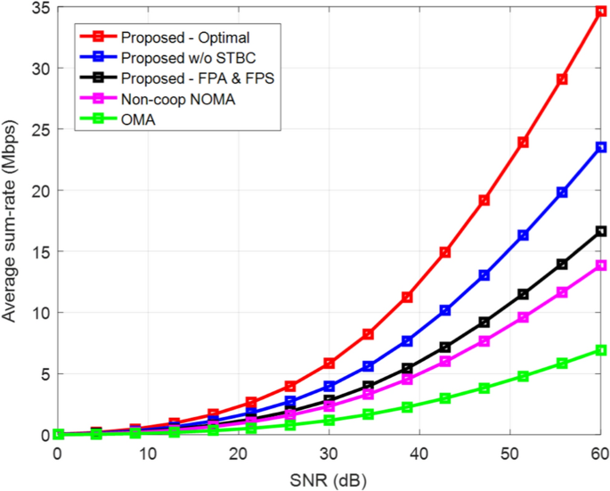

  

  Average sum-rate versus SNR

• (2) Achievable rate versus SNR: Aside from the system sum-rate, it is also important to investigate the individual achievable rate of the users in the network. The individual achievable rate can be used in the tuning of transmission parameters such as power allocation factor and power splitting ratio in order to achieve fairness among users. Thus, in Fig. 4, the achievable rate of each user in the STBC group is depicted based on the expressions in (12), (13), (35), and (36).

  Fig. 4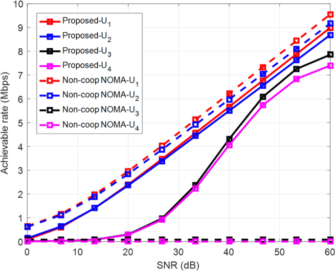

  

  Achievable rate versus SNR

  Furthermore, we compare our results with the case where the system operates non-cooperative NOMA. According to the proposed algorithm 2, the system degenerates into non-cooperative NOMA when the harvested power threshold is not satisfied, i.e., when $\tilde{P}_{k} < P_{h_{min}}$. We observe that the achievable rates of $U_1$ and $U_2$ increase throughout the entire SNR region. However, at the low SNR region (below approximately 13 dB), $U_3$ and $U_4$ are in complete outage, and the curve tends to be bounded at the high SNR region. The reason for these characteristics can be associated with the absence of a direct path from the source to $U_3$ and $U_4$ and the adoption of the non-linear harvested energy model in (11). Since $U_1$ and $U_2$ rely on the harvested power to forward the information of $U_3$ and $U_4$, a significant increase in their rate is only possible when the EH circuits operate in the linear region. For the non-cooperate case, as expected, the achievable rates of $U_1$ and $U_2$ perform slightly better than the proposed solution since the harvested power in this case is considered very small; consequently, all the allocated power is used for information transmission. Hence, based on these findings, we recommend that the system be designed around an SNR value that will enable the EH relays to operate in a linear region which in our case is 13 dB.

• (3) Average achievable sum-rate versus number of users: Here, we study the effect of varying numbers of users on the system resources and its impact on the average sum-rate of the system. As depicted in Fig. 5, we evaluate the average system sum-rate for different numbers of users at an SNR of 30 dB. The 30 dB SNR value is chosen for illustration purposes since a notable rise in the achievable rate of the FUE (i.e., $U_3$ and $U_4$) is observed at this point as presented in Fig. 4.

  Fig. 5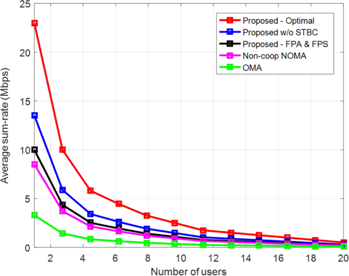

  

  Average sum-rate versus number of users, where SNR = 30 dB, $R_{min} = 1$ Mbps

  We observe that the average sum-rate of the system decreases with an increasing number of users. The main reason behind this lies in the fact that the power allocation factor of each user decreases with an increasing number of users. Moreover, according to power allocation in the PD-NOMA scheme, the users in the NUE set are allocated small power values compared with those in FUE set. This in turn reduces their ID and EH rates since both depend on the allocated power. Though our proposed solution still outperforms the benchmark scheme, additional improvement can be achieved by increasing the SNR range. However, this may come at the cost of higher transmission power at the source, which may degrade the energy efficiency of the system.

• (4) Optimal power allocation factor versus SNR: In Fig. 6, we investigate the effect of optimal values of power allocation factor of the NUE relays under different transmission SNR values.

  Fig. 6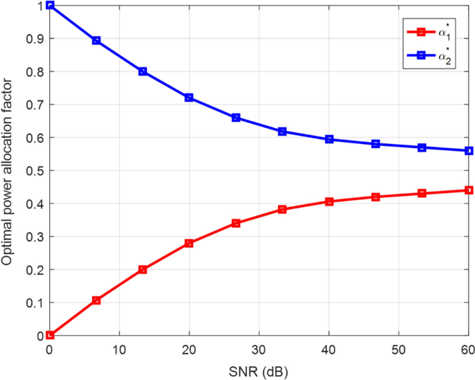

  

  Optimal power allocation factor versus SNR

  We observe that with increasing SNR, the values of optimal power allocation factors $\alpha _{1}^{*}$ and $\alpha _{2}^{*}$ tend to converge toward the same value. The reason for this can be attributed to the fact that at higher SNR values, channel impairments become suppressed. Hence, the difference between the power allocated to the users at the transmitter becomes smaller and approaches the same value in order to maintain fairness. Hence, for efficient system design, the transmission power of the source should be designed around the SNR values at the convergence points of the power allocation factors.

• (5) Optimal power splitting ratio versus SNR: In Fig. 7, we investigate the effect of optimal values of power splitting ratio of the NUE relays under different transmission SNR values.

  Fig. 7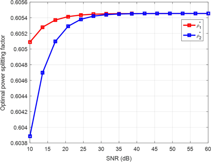

  

  Optimal power splitting ratio versus SNR

  With increasing SNR, we observe that the optimal power splitting ratios $\rho _{1}^{*}$ and $\rho _{2}^{*}$ converge towards the same value, which is approximately 0.61. The convergence of these values ensures that at higher SNR, the optimal power splitting ratios for the information decoding rate ($1-\rho _{k}, k \in \{1,2\}$) given in (5) and (9) are not violated. Moreover, for the proposed solution we can infer, that the optimal transmission power of the source can be achieved at an SNR value corresponding to the convergence point of the optimal power splitting ratios, which is approximately 40 dB.

• (6) Energy efficiency versus transmission power: In Fig. 8, the energy efficiency of the developed system is evaluated.

  Fig. 8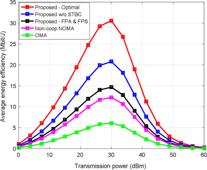

  

  Energy efficiency versus transmission power

  It can be seen that the energy efficiency of our proposed solution has the best overall performance. This can also be attributed to the improved rate offered by the STBC transmission. Another critical observation is the existence of an upper bound for all the evaluated cases. This could be the effect of saturation characteristics of non-linear EH and the impact of other circuit constants. Note that the NUEs adopted a non-linear energy harvesting model, as presented in (11). At saturation, the NUE transmission power (which is the energy harvesting UE) becomes constant. Though their rate should be constant as well, with increasing source transmission power and power consumption of other circuit components (which are part of the denominator functions in (56)), the sum-rate of the system (which is the numerator function) will start decreasing. Consequently, the reason for the decline in energy efficiency of the system. However, the upper bound limit can be extended by increasing the values of the power spitting ratios $\rho _1$ and $\rho _2$ to minimize the effect of energy consumption in the system. Nonetheless, this will come at the cost of a lower achievable rate. Therefore, to ensure an energy-efficient system design, the transmission power that maximizes the average system sum-rate must be taken into account.

• (7) Average sum-rate versus number of iterations: To evaluate the computational complexity of the proposed algorithms, we present the number of iterations required to achieve convergence in terms of the system sum-rate. As depicted in Fig. 9, the convergence rate of the proposed optimization algorithm is presented with respect to different achievable rate thresholds.

  Fig. 9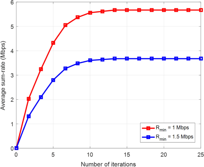

  

  Average sum-rate versus number of iterations for different rate thresholds, where SNR = 30 dB

  We observe that the average sum-rate of the system converges after approximately 10 iterations, which translates to the low computational complexity of our proposed solution. Furthermore, we observe a decrease in the system achievable rate when the minimum rate $R_{min}$ is increased to 1.5 Mbps. The reason for this can be associated with the fact that the power splitting ratio $\rho _{k}$ used by $U_1$ and $U_2$ in (1) has to be reduced such that the ID rate can satisfy the system rate threshold. However, this comes at the cost of smaller harvested energy, which in turn minimizes the transmission rate to $U_3$ and $U_4$. Thus, we can infer that at higher rate thresholds, the system sum-rate is dominated by contributions from the NUEs.

6 Conclusions

In this study, we have examined the performance of an STBC-aided C-NOMA system with RF energy harvesting capacity from the standpoint of average sum-rate maximization and energy efficiency. To achieve this, we incorporate a user pairing scheme that can be generalized for the establishment of multiple STBC groups. Moreover, we employ the non-linear energy harvesting model at the near-field user pair to alleviate the energy consumption problem during the STBC cooperative transmission phase. Further to this, we develop a low-complexity solution based on the concepts of the Stackelberg game and Nash the bargaining solution. Based on this, we develop an iterative algorithm that jointly optimizes the power allocation and power splitting ratios. The outcome of our findings shows that joint consideration of STBC and energy harvesting in C-NOMA networks with dynamic power allocation and power splitting ratios achieves better performance than the baseline schemes. In the future, we aim to extend this study by developing a more robust user pairing scheme in which a channel gain constraint is included in the user grouping. In addition, we shall consider the impact of full-duplex transmission, imperfect SIC and channel uncertainties.

References

San Jose, C. A., & Cisco, U. (2020). Cisco annual internet report (2018–2023) white paper (pp. 1–35). USA: Cisco.
Alamu, O., Iyaomolere, B., & Abdulrahman, A. (2021). An overview of massive MIMO localization techniques in wireless cellular networks: Recent advances and outlook. Ad Hoc Networks, 111, 102353.
Liu, Y., et al. (2022). Evolution of NOMA toward next generation multiple access (NGMA) for 6G. IEEE Journal on Selected Areas in Communications, 40, 1037–1071.
Abd-Elnaby, M., Sedhom, G. G., El-Rabaie, E.-S.M., & Elwekeil, M. (2023). NOMA for 5G and beyond: Literature review and novel trends. Wireless Networks, 29, 1629–1653.
Maraqa, O., Rajasekaran, A. S., Al-Ahmadi, S., Yanikomeroglu, H., & Sait, S. M. (2020). A survey of rate-optimal power domain NOMA with enabling technologies of future wireless networks. IEEE Communications Surveys & Tutorials, 22, 2192–2235.
Soni, S., Makkar, R., Rawal, D., & Sharma, N. (2023). Performance analysis of selective DF cooperative NOMA in presence of practical impairments. IEEE Systems Journal, 17(3), 4545–4554.
Merin Joshiba, J., Judson, D., & Bhaskar, V. (2023). A comprehensive review on NOMA assisted emerging techniques in 5G and beyond 5G wireless systems. Wireless Personal Communications, 130, 1–21.
Alamu, O., Olwal, T. O., & Djouani, K. (2024). Cooperative visible light communications: An overview and outlook. Optical Switching and Networking, 29, 100772.
Liaqat, M., Noordin, K. A., Abdul Latef, T., & Dimyati, K. (2020). Power-domain non orthogonal multiple access (PD-NOMA) in cooperative networks: An overview. Wireless Networks, 26, 181–203.
Alamouti, S. M. (1998). A simple transmit diversity technique for wireless communications. IEEE Journal on Selected Areas in Communications, 16, 1451–1458.
Murata, H., Kuwabara, A., & Oishi, Y. (2021). Distributed cooperative relaying based on space-time block code: System description and measurement campaign. IEEE Access, 9, 25623–25631.
Alamu, O., Olwal, T. O., & Djouani, K. (2023). Cooperative NOMA networks with simultaneous wireless information and power transfer: An overview and outlook. Alexandria Engineering Journal, 71, 413–438.
Toulouse, M., Dai, H., & Le, T. G. (2022). Distributed load-balancing for account-based sharded blockchains. International Journal of Web Information Systems, 18, 100–116.
Gao, H., et al. (2023). TBDB: Token bucket-based dynamic batching for resource scheduling supporting neural network inference in intelligent consumer electronics. IEEE Transactions on Consumer Electronics, 70(1), 1134–1144.
Gao, H., Wang, X., Wei, W., Al-Dulaimi, A., & Xu, Y. (2023). Com-DDPG: Task offloading based on multiagent reinforcement learning for information-communication-enhanced mobile edge computing in the internet of vehicles. IEEE Transactions on Vehicular Technology, 73(1), 348–361.
Zhang, Z., Hu, Q., Hou, G., & Zhang, S. (2023). A real-time discovery method for vehicle companion via service collaboration. International Journal of Web Information Systems, 19, 263–279.
Yang, X., Xu, Y., Zhou, Y., Song, S., & Wu, Y. (2022). Demand-aware mobile bike-sharing service using collaborative computing and information fusion in 5G IoT environment. Digital Communications and Networks, 8, 984–994.
Alamu, O., Gbenga-Ilori, A., Adelabu, M., Imoize, A., & Ladipo, O. (2020). Energy efficiency techniques in ultra-dense wireless heterogeneous networks: An overview and outlook. Engineering Science and Technology, An International Journal, 23, 1308–1326.
Alamu, O., Olwal, T. O., & Djouani, K. (2022). Simultaneous lightwave information and power transfer in optical wireless communication networks: An overview and outlook. Optik, 266, 169590.
Alamu, O., Olwal, T. O., & Djouani, K. (2023). Energy harvesting techniques for sustainable underwater wireless communication networks: A review. e-Prime-Advances in Electrical Engineering, Electronics and Energy, 4, 100265.
Alamu, O., Olwal, T. O., & Djouani, K. (2022). An overview of simultaneous wireless information and power transfer in massive MIMO networks: A resource allocation perspective. Physical Communication, 57, 101983.
Yang, K., Yan, X., Wang, Q., Jiang, D., & Qin, K. (2021). DSWIPT scheme for cooperative transmission in downlink NOMA system. Mobile Networks and Applications, 26, 609–619.
Tran, H. Q., Vien, Q.-T., et al. (2023). SWIPT-based cooperative NOMA for two-way relay communications: PSR versus TSR. Wireless Communications and Mobile Computing, 2023, 3069999.
Ghosh, S., Al-Dweik, A., & Alouini, M.-S. (2023). On the performance of end-to-end cooperative NOMA-based IoT networks with wireless energy harvesting. IEEE Internet of Things Journal, 10(8), 16253–16270.
Khennoufa, F., Khelil, A., Rabie, K., Kaya, H., & Li, X. (2023). An efficient hybrid energy harvesting protocol for cooperative NOMA systems: Error and outage performance. Physical Communication, 58, 102061.
Khennoufa, F., Abdellatif, K., & Kara, F. (2022). Bit error rate evaluation of relay-aided cooperative NOMA with energy harvesting under imperfect SIC and CSI. Physical Communication, 52, 101630.
Le, T. A., & Kong, H. Y. (2020). Performance analysis of downlink NOMA-EH relaying network in the presence of residual transmit RF hardware impairments. Wireless Networks, 26, 1045–1055.
Hoang, T. M., Thang, N. N., Nguyen, B. C., & Tran, P. T. (2022). Enhancing the performance of downlink NOMA relaying networks by RF energy harvesting and data buffering at relay. Wireless Networks, 28, 1857–1877.
Özgün, E., & Aygölü, Ü. (2022). Energy harvesting in ARQ-based cooperative broadcast and NOMA networks. Wireless Networks, 26, 1–14.
Zaidi, S. K., Hasan, S. F., & Gui, X. (2020). Two-way SWIPT-aided hybrid NOMA relaying for out-of-coverage devices. Wireless Networks, 26, 2255–2270.
Wu, M., Song, Q., Guo, L., & Jamalipour, A. (2021). Joint user pairing and resource allocation in a SWIPT-enabled cooperative NOMA system. IEEE Transactions on Vehicular Technology, 70, 6826–6840.
Hoang, T. M., Tan, N. T., Hoang, N. H., & Hiep, P. T. (2019). Performance analysis of decode-and-forward partial relay selection in NOMA systems with RF energy harvesting. Wireless Networks, 25, 4585–4595.
Ren, Y., et al. (2023). Impartial cooperation in SWIPT-assisted NOMA systems with random user distribution. IEEE Transactions on Vehicular Technology, 72, 10488–10504.
Parihar, A. S., Swami, P., Bhatia, V., & Ding, Z. (2021). Performance analysis of SWIPT enabled cooperative-NOMA in heterogeneous networks using carrier sensing. IEEE Transactions on Vehicular Technology, 70, 10646–10656.
Parihar, A. S., Swami, P., & Bhatia, V. (2022). On performance of SWIPT enabled PPP distributed cooperative NOMA networks using stochastic geometry. IEEE Transactions on Vehicular Technology, 71, 5639–5644.
Lei, R., Xu, D., & Ahmad, I. (2021). Secrecy outage performance analysis of cooperative NOMA networks with SWIPT. IEEE Wireless Communications Letters, 10, 1474–1478.
Nguyen, V.-L., Ha, D.-B., Truong, V.-T., Tran, D.-D., & Chatzinotas, S. (2022). Secure communication for RF energy harvesting NOMA relaying networks with relay-user selection scheme and optimization. Mobile Networks and Applications, 27, 1719–1733.
Hu, C., Li, Q., Zhang, Q., & Qin, J. (2022). Security optimization for an AF MIMO two-way relay-assisted cognitive radio nonorthogonal multiple access networks with SWIPT. IEEE Transactions on Information Forensics and Security, 17, 1481–1496.
Vu, T.-H., Nguyen, T.-V., & Kim, S. (2021). Cooperative NOMA-enabled SWIPT IoT networks with imperfect SIC: Performance analysis and deep learning evaluation. IEEE Internet of Things Journal, 9, 2253–2266.
Nguyen, M.-T., Vu, T.-H., & Kim, S. (2022). Performance analysis of wireless powered cooperative NOMA-based CDRT IoT networks. IEEE Systems Journal, 16, 6501–6512.
Aswathi, V., & Babu, A. V. (2021). Outage and throughput analysis of full-duplex cooperative NOMA system with energy harvesting. IEEE Transactions on Vehicular Technology, 70, 11648–11664.
Nguyen, T.-T., Nguyen, S. Q., Nguyen, P. X., & Kim, Y.-H. (2022). Evaluation of full-duplex SWIPT cooperative NOMA-based IoT relay networks over Nakagami-m fading channels. Sensors, 22, 1974.
Liu, C., Zhang, L., Chen, Z., & Li, S. (2022). Outage probability analysis in downlink SWIPT-assisted cooperative NOMA systems. Journal of Communications and Information Networks, 7, 72–87.
Aldababsa, M. (2023). Performance of TAS/MRC in NOMA energy harvesting relay networks. AEU-International Journal of Electronics and Communications, 162, 154569.
Le, T. A., & Kong, H. Y. (2020). Energy harvesting relay-antenna selection in cooperative MIMO/NOMA network over Rayleigh fading. Wireless Networks, 26, 2075–2087.
Ren, J., Lei, X., Peng, Z., Tang, X., & Dobre, O. A. (2022). RIS-assisted cooperative NOMA with SWIPT. IEEE Wireless Communications Letters, 12(3), 446–450.
Zhao, J., Ding, Z., Fan, P., Yang, Z., & Karagiannidis, G. K. (2018). Dual relay selection for cooperative NOMA with distributed space time coding. IEEE Access, 6, 20440–20450.
Akhtar, M. W., Hassan, S. A., Saleem, S., & Jung, H. (2020). STBC-aided cooperative NOMA with timing offsets, imperfect successive interference cancellation, and imperfect channel state information. IEEE Transactions on Vehicular Technology, 69, 11712–11727.
Zhai, C., Li, Y., Wang, X., Zheng, L., & Li, C. (2023). Wireless powered cooperative NOMA with Alamouti coding and selection relaying. IEEE Transactions on Mobile Computing, 23(2), 1366–1381.
Demirkol, B., Toka, M., & Kucur, O. (2023). Outage performance of NOMA with Alamouti/MRC in dual-hop energy harvesting relay networks. Physical Communication, 58, 102026.
Alamu, O., Olwal, T. O., & Djouani, K. (2023). Achievable rate optimization for space-time block code-aided cooperative NOMA with energy harvesting. Engineering Science and Technology, An International Journal, 40, 101365.
Gao, H. (2023). Cloud-edge intelligence collaborative computing: Software, communication and human. Mobile Networks and Applications, 27, 1–3.
Singh, S. K., Agrawal, K., Singh, K., Li, C.-P., & Alouini, M.-S. (2022). Noma enhanced UAV-Assisted communication system with nonlinear energy harvesting. IEEE Open Journal of the Communications Society, 3, 936–957.
Tran, T.-N., Voznak, M., Fazio, P., & Ho, V.-C. (2021). Emerging cooperative MIMO-NOMA networks combining TAS and SWIPT protocols assisted by an AF-VG relaying protocol with instantaneous amplifying factor maximization. AEU-International Journal of Electronics and Communications, 135, 153695.
Osborne, M. J., & Rubinstein, A. (1990). Bargaining and markets. USA: Academic Press Limited.
Han, Z., Niyato, D., Saad, W., Başar, T., & Hjørungnes, A. (2012). Game theory in wireless and communication networks: Theory, models, and applications. Cambridge: Cambridge University Press.
Shao, X., Yang, C., Chen, D., Zhao, N., & Yu, F. R. (2018). Dynamic IoT device clustering and energy management with hybrid NOMA systems. IEEE Transactions on Industrial Informatics, 14, 4622–4630.
Huang, H., & Zhu, M. (2019). Energy efficiency maximization design for full-duplex cooperative NOMA systems with swipt. IEEE Access, 7, 20442–20451.
Su, B., Ni, Q., & Yu, W. (2019). Robust transmit beamforming for SWIPT-enabled cooperative NOMA with channel uncertainties. IEEE Transactions on Communications, 67, 4381–4392.
Zhang, Z., Qu, H., Zhao, J., & Wang, W. (2021). Contract theory-based incentive mechanism for full duplex cooperative NOMA with Swipt communication networks. Entropy, 23, 1161.
Funding
Open access funding provided by Tshwane University of Technology. This research was funded by the Telkom-CoE and the National Research Foundation (NRF) of South Africa (Grant Number: 90604). Opinions, findings, and conclusions or recommendations expressed in any publication generated by NRF-supported research are those of the author(s) alone, and the NRF accepts no liability whatsoever in this regard.
Author information
Authors and Affiliations
Contributions
Olumide Alamu: Conceptualization, System model design and analysis, Interpretation of results, Writing the original manuscript draft. Thomas O. Olwal: Conceptualization, Supervision, Revision and editing the manuscript, Funding acquisition. Karim Djouani: Conceptualization, Supervision, Revision and editing the manuscript, Funding acquisition.
Corresponding author
Ethics declarations
Conflict of interest
The authors declare that they have no known competing financial interests or personal relationships that could have appeared to influence the work reported in this paper.
Ethical approval
Not Applicable.
Additional information
Publisher's Note
Springer Nature remains neutral with regard to jurisdictional claims in published maps and institutional affiliations.
Rights and permissions
Open Access This article is licensed under a Creative Commons Attribution 4.0 International License, which permits use, sharing, adaptation, distribution and reproduction in any medium or format, as long as you give appropriate credit to the original author(s) and the source, provide a link to the Creative Commons licence, and indicate if changes were made. The images or other third party material in this article are included in the article's Creative Commons licence, unless indicated otherwise in a credit line to the material. If material is not included in the article's Creative Commons licence and your intended use is not permitted by statutory regulation or exceeds the permitted use, you will need to obtain permission directly from the copyright holder. To view a copy of this licence, visit http://creativecommons.org/licenses/by/4.0/.
About this article
Cite this article
Alamu, O., Olwal, T.O. & Djouani, K. Sum-rate maximization for a distributed space-time block code-aided cooperative NOMA with energy harvesting. Wireless Netw (2024). https://doi.org/10.1007/s11276-024-03757-7
Accepted:
Published:
DOI: https://doi.org/10.1007/s11276-024-03757-7