
Abstract
Spatial accuracy of hydrologic modeling inputs influences the output from hydrologic models. A pertinent question is to know the optimal level of soil sampling or how many soil samples are needed for model input, in order to improve model predictions. In this study, measured soil properties were clustered into five different configurations as inputs to the Soil and Water Assessment Tool (SWAT) simulation of the Castor River watershed (11-km2 area) in southern Quebec, Canada. SWAT is a process-based model that predicts the impacts of climate and land use management on water yield, sediment, and nutrient fluxes. SWAT requires geographical information system inputs such as the digital elevation model as well as soil and land use maps. Mean values of soil properties are used in soil polygons (soil series); thus, the spatial variability of these properties is neglected. The primary objective of this study was to quantify the impacts of spatial variability of soil properties on the prediction of runoff, sediment, and total phosphorus using SWAT. The spatial clustering of the measured soil properties was undertaken using the regionalized with dynamically constrained agglomerative clustering and partitioning method. Measured soil data were clustered into 5, 10, 15, 20, and 24 heterogeneous regions. Soil data from the Castor watershed which have been used in previous studies was also set up and termed “Reference”. Overall, there was no significant difference in runoff simulation across the five configurations including the reference. This may be attributable to SWAT's use of the soil conservation service curve number method in flow simulation. Therefore having high spatial resolution inputs for soil data may not necessarily improve predictions when they are used in hydrologic modeling.
1 Introduction
Spatial heterogeneity of soil properties in hydrologic and water quality models is often ignored or rarely taking into consideration in the management of freshwater resources (Steinman and Denning 2005). Heterogeneity of soil and land processes contributes to all aspects of the hydrologic cycle (Tague 2005). Having an understanding of the types and processes of spatial heterogeneity is a fundamental component of both theoretical and applied hydrology (Tague 2005). In other words, incorporation of spatial heterogeneity into hydrologic and water quality models should provide a new way to view water quality prediction and freshwater management. This should lead to potentially useful management strategies (Steinman and Denning 2005).
In water quality predictions, there is a need for good nutrient management plans, along with monitoring and decision support systems for nonpoint sources control. Daily or weekly sampling techniques of soil and water variables are technically feasible but not economical. Therefore, there is a need for good prediction models which take spatial watershed variability into account to aid in this circumstance.
One of the most widely applied hydrologic and water quality models is the Soil and Water Assessment Tool (SWAT), developed by the US Department of Agriculture (Arnold et al. 1998). SWAT needs spatial inputs such as a digital elevation model (DEM) as well as land use and soil maps. The modeling procedure and various applications can be found in Arnold et al. (1998) and Gassman et al. (2007). There is a major challenge in the application of this model: the representation of soil heterogeneities. The Hydrologic Response Unit (HRU) is a virtual but unique homogeneous classification of units (areas) of similar land-use, soil class and slope. These units are then aggregated together to form a sub-basin. Each sub-basin drains into a stream which exits to a main drainage waterway. The assumption is that spatial distributions of soil properties are preserved in HRUs; however, in the soil database, the soil classes use mean values for all soil properties. Therefore, the spatial variations of these properties are not completely represented in SWAT.
Given the foregoing, the aim of this research is to quantify the impact of incorporating spatial variability and heterogeneity of soil properties into SWAT, specifically in terms of predicting runoff, sediment, and total phosphorus (TP) loss from agricultural fields. This paper is the first of two regarding the quantification of the impacts of soil heterogeneities on prediction of runoff, sediment, and P loss to Missisquoi Bay. The second paper will involve the quantification of heterogeneities (of other watershed features such as land use) and the sensitivities of SWAT configurations to long-term predictions of runoff, sediment, and TP loss.
2 Materials and Methods
2.1 Study Watershed Description
Castor watershed (45°08′N, 72°58′W, 11-km2 area), a sub-watershed of the Pike River, is located near the town of Bedford in southern Quebec, Canada (Fig. 1). The Pike River watershed drains into Missisquoi Bay (northeastern portion of Lake Champlain). There is a great deal of evidence that the eutrophication seen in the Bay is due to excess nutrient losses from agricultural watersheds (Hegman et al. 1999; Jamieson et al. 2003; Deslandes et al. 2004; Medalie and Smeltzer 2004). This is a serious challenge from a water quality perspective.

The study area and sample points
Castor watershed's landscape ranges from 36 to 49 m of elevation above sea level. There is a transition gradient from low, poorly drained lacustrine clays to loamy glacial calcareous tills (Michaud 2004). This result in low water infiltration and poor drainage, which along with wet antecedent moisture conditions and snow melt have contributed to flooding events in recent years. Consequently, sub-surface drains are installed on most farms to remove excess water from agricultural fields. The water table in this region is reported to be shallow (Deslandes et al. 2007). The mean long-term annual precipitation (1971–2007) of this study area is about 1,057 mm (Michaud 2004). The watershed is an area of intensive agricultural activity, where land is cropped 44 % to corn (Zea mays L.), 28 % to grass (hay), and 20 % to cereals. Other agricultural operations such as swine, poultry, and dairy production make up the remaining 8 % (Deslandes et al. 2007).
The major soil series of the watershed are as follows (Michaud 2004):
-
Ste. Rosalie: poorly drained lacustrine and marine clays
-
Bedford: an Orthic Humic Gleysol, fine loamy mixed calcareous
-
Ste. Brigide: an Orthic Humic Gleysol, Coarse-loamy mixed calcareous
-
St. Sebastien: Gleyed Sombric Brunisol, loamy-skeletal, mixed, monoacid, mesic
2.2 Field Measurements and Laboratory Analysis of Soil Properties
A stratified random soil sampling of the study area was also completed (Fig. 1). Soil samples (at depths 0–0.30, 0.30–0.60, and 0.60–0.90 m) were collected. SWAT soil database requires the following soil physical properties (Neitsch et al. 2009):
-
Soil bulk density (SOL_BD). This quantity measures soil compaction. Among the factors that influence SOL_BD include volumetric water content, hydraulic conductivity, soil water content, and soil porosity. The core samples were weighed and oven dried to constant weight at 105 °C. SOL_BD was calculated as (Neitsch et al. 2009)
$$ \rho =\frac{\left({M}_W-{M}_D\right)}{V} $$(1)where ρ is the bulk density (g cm−3), M W is the weight of wet soil (before oven dry) (g), W D is the weight of dry soil (after oven dry) (g), and V is the volume of soil core in (cm3).
-
Particle size distribution (SOL_CLAY, SOL_SILT, and SOL_SAND). Hydrometer method was used to analyze the percentage of clay, sand and silt (Neitsch et al. 2009; Somenahally et al. 2009). The unit is percentage of soil by weight.
-
Soil organic carbon (SOL_CBN). Soil organic matter is related to soil stability, structure, fertility, and nutrient retention. The loss-on-ignition procedure was used. This is based on the concept of using a very high temperature to convert the carbon to carbon dioxide. A soil mass of about 20 to 30 g was used for this process (Neitsch et al. 2009; Prasad and Power 1997; Donkin 1991). The unit is percentage of soil weight.
-
Available water content (SOL_AWC). This is calculated as the difference between the fraction of water present at wilting point and that present at field capacity. A pressure plate device was used to estimate the soil field capacity and permanent wilting point. We determined the field capacity (ψ fc) as the amount of water content at a soil matric potential of −0.033 bars. The permanent wilting point (ψ pwp) was determined as the water content at a soil matric potential of −15 bars (Neitsch et al. 2009; Burk and Dalgliesh 2008). The unit is millimeter water per millimeter soil (mm H2O mm−1 soil).
-
Universal soil loss equation’s soil erodibility factor (K) (USLE_K ). This quantifies how one soil is more erodible than another when all other factors are the same (the unit is 0.013 Mg m2 h) / m3–Mg cm). This can also be defined as the soil loss rate per erosion index unit for a specified soil as measured on a unit plot (Neitsch et al. 2009; Wischmeier and Smith 1978). The procedure suggested by (Neitsch et al. 2009) was used to derive the USLE_K.
-
Hydraulic conductivity (SOL_K) (mm h − 1 ). The mean soil texture in this study area is fine textured; therefore, the falling-head method was used to measure the soil permeability characteristics. The falling-head permeability test was used (Bowles 1986).
2.3 Spatial Clustering and Discretization of Soil Polygons
To account for spatial heterogeneity in soil properties, actual soil values instead of averages should be used. Therefore, clustering of the measured point set data was performed. This will provide the platform and the ability to define any desired number of spatial objects (soil polygons). This was done through the following procedures:
-
1.
The Thiessen polygon tool in ArcGIS software 10 (Environmental Systems Research Institute, Redlands, CA, USA) was used to divide the area covered by each sample point (input feature) into Thiessen or proximal zones (Guo 2008). These proximal polygons are very important in aggregation and division of sample points into desired heterogeneous regions. This process divided the study area into triangulated irregular networks that we considered heterogeneous. The concept of a Thiessen polygon is defined as a process where D is a set of points in coordinate or Euclidean space (x, y). For any point k in that space, there is one point of D closest to k, except where point k is equidistant to two or more points of D (ESRI 2012).
-
2.
As clustering these individual proximal zones was of interest, regionalization with dynamically constrained agglomerative clustering and partitioning (REDCAP) technique was implemented (Guo 2008; Bernassi and Ferrara 2010). Regionalization is very important in dividing spatial objects (proximal polygons) into a number of spatially contiguous regions. A full-order complete-linkage clustering (CLK) technique (Guo 2008) was used to derive heterogeneous clustered regions. This procedure involved two steps:
-
1)
Clustering the data with contiguous constraints to produce spatially contiguous trees or hierarchy, and
-
2)
Partitioning the tree to generate regions while optimizing an objective function
According to Guo (2008), the CLK defines the distance between two clusters as the dissimilarity between the farthest pair of points as
$$ {X}_{\mathrm{CLK}}\left(P,R\right)={\mathrm{Max}}_{a\in P,b\in R}\left({X}_{a,b}\right), $$(2)where P and R are two clusters, a ∈ P and b ∈ R are the data points, and X a,b is the dissimilarity between a and b.
Guo (2008) defined full-order constraining strategies as a clustering process where all edges are included in the process. The advantage of using full order over the first order is that the full-order strategy is dynamic and it updates the contiguity matrix after each merge (Guo 2008). This method produces different trees (Guo 2008), which therefore define different search methods for the partitioning. Thereafter, the partitioning of the contiguous tree will produce a number of sub-trees, each of which corresponds to a contiguous region (Bernassi and Ferrara 2010). The partitioning is iteratively done to partition a spatial contiguous tree into a number of regions by cutting a sub-tree (Guo 2008; Bernassi and Ferrara 2010). The following equation gives the homogeneity gain. This can also be called heterogeneity reduction. The best sub-tree to cut at each step is the sub-tree with the largest homogeneity expressed as
$$ {h}_g^{\ast }(k)= \max \left[L\left({K}_a\right)-L\left({K}_b\right)\right] $$(3)where K a and K b are the two sub-trees from a possible cut of K and h g * is the homogeneity gain for the tree after the best cut (Guo 2008; Bernassi and Ferrara 2010).
The sum of square deviation (SSD), which can be used as the heterogeneity measure, is expressed as (Guo 2008)
$$ L(K)={\displaystyle \sum \frac{s}{h=1}}{\displaystyle \sum \frac{n_r}{g=1}}{\left({x}_{hg}-{\gamma}_h\right)}^2 $$(4)where n r is the number of objects in region K, x gh is the value for the hth attribute of the gth object, γ h is the mean value of the hth attribute for all objects, K is a region, L(K) is the heterogeneity, and S is the number of attributes.
Therefore, the total heterogeneity, L k , for a regionalization result with k regions can be given as the total of the k heterogeneity values (Guo 2008):
$$ {L}_k={\displaystyle \sum \frac{k}{h=1}L\left({K}_h\right)} $$(5) -
1)
-
3.
From the foregoing, we partitioned the proximal zones (from (1) using the procedure explained in (2)) into 5, 10, 15, 20, and 24 heterogeneous clusters, termed “Region_5”, “Region_10”, “Region_15”, “Region_20”, and “Region_24”, respectively.
-
4.
We used the normal soil map with average properties that have been used in several studies (Deslandes et al. 2007; Michaud et al. 2008) in the watershed as the sixth configuration termed “Reference”.
2.4 SWAT Model Setup
The SWAT model was selected for this project because of its worldwide applications (Gassman et al. 2007). SWAT2009 being the most stable recent version was selected along with an AVSWAT interface combined with ArcView 3.3.
SWAT requires several inputs such as a digital elevation model (DEM), land use, and soil characteristics. Some climatic variables are also needed: daily rainfall, relative humidity, temperature, etc. All spatial inputs (DEM, soil (termed Reference later) and land use) were obtained from the Institut de Recherche et de Développement en Agroenvironment. DEM has a spatial resolution of 30 m, accurate to approximately ±1.3 m (Michaud et al. 2008). The climatological data was derived from the three closest weather stations (Philipsburg, Farnham, and Sutton) in the area (MDDEPQ 2003, 2005). Based on previous hydrologic modeling done in the area using SWAT (Michaud et al. 2008), a recommended value of 31 mg kg−1 was adopted for the initialized labile P soil concentration.
A sub-surface drainage of approximate 60 % for cultivated land, mean drain depth of 0.900 m, time required to achieve field capacity of 48 h, and drainage time into waterways of 18 h were assumed for the study area (Michaud et al. 2008).
Finally, we set up six SWAT model scenarios using the different soil configurations:
-
1.
Reference. This was the SWAT model setup using soil map that has been used for previous studies in the study area. We call this reference because it is based on average values of soil properties.
-
2.
Region_5. This was a SWAT configuration setup using the survey soil properties partitioned into five heterogeneous regions.
-
3.
Region_10. This is a SWAT configuration setup using the survey soil properties partitioned into ten heterogeneous regions.
-
4.
Region_15. This is a SWAT configuration setup using the survey soil properties partitioned into 15 heterogeneous regions.
-
5.
Region_20. This is a SWAT configuration setup using the survey soil properties partitioned into 20 heterogeneous regions.
-
6.
Region_24. This is a SWAT configuration setup using the survey soil properties partitioned into 24 heterogeneous regions. In other words, in this configuration, each unit (sampled points) is a region in itself.
2.5 Evaluating Model
The model's output was obtained as a monthly time step. The model's performance was assessed using the coefficient of determination (R 2) and the Nash–Sutcliffe efficiency (NSE) (Nash and Sutcliffe 1970). The R 2 is a statistical index which varies from 0 to 1, where R 2 = 1.0 indicates that the correspondence between the predicted and observed perfectly fits a linear relationship. The NSE also ranges from −∞ to 1. An NSE of 1 indicates a perfect fit between the predicted and observed values, whereas an NSE of 0 represents predictions that are only as accurate as the mean of the observed data. When the NSE is less than zero, then the observed mean is a better predictor than the model. The simulation period was from January 1971 to December 2007. The periods from January 1971 to December 1976 (5 years) were used as a warm-up period. This is done to allow the model to “stabilize”, especially for model parameters such as soil moisture where they are dependent on prior conditions. The time periods from April 2001 to December 2002 were used for the evaluation of flow, sediment, and TP fluxes (before and after calibration). Observed discharges, suspended sediments, and TP data sets were obtained from the Ministère du Développement durable, Environnement et Parcs du Quebec (MDDEPQ 2003, 2005).
3 Results and Discussion
3.1 Descriptive Statistics of the Measured Soil Properties
Descriptive statistics of surveyed soil properties SOL_BD, SOL_CLAY, SOL_SILT, SOL_SAND, SOL_CBN, SOL_AWC, and SOL_K are presented in Tables 1, 2, and 3 for soil depths of 0–0.30, 0.30–0.60, and 0.60–0.90 m, respectively. The parameter ranges are within the acceptable ranges required by SWAT (Neitsch et al. 2009). In examining the coefficient of variation for the three depths, SOL_K and SOL_CLAY were found to have the highest variability, while SOL_BD has the lowest. This is consistent with findings from the literature concerning soil permeability and bulk density.
3.2 Soil Clustering Analysis, Partitioning, and Regionalization
The result of the spatial division of the study area into 24 polygons using the Thiessen polygon technique in ArcGIS 10 is illustrated in Fig. 2. Each polygon has unique soil properties. We clustered these proximal zones into 24, 20, 15, 10, and 5 heterogeneous zones. The clusters and derived soil maps can be seen in Figs. 3, 4, and 5. Within-region heterogeneity of each of the regions is shown in Fig. 6. The SSD measure of within-region heterogeneity indicated that the configurations with the least number of regions (Region_5) were the most heterogeneous while the lowest SSD value was found for Region_24. In other words, the smallest SSD value was obtained when each unit (sample point) was a region in itself. This makes the region mean the same as the unit mean. Therefore, the greater number of regions, the less heterogeneous the region is. These maps were used as soil inputs into SWAT to quantify the impact of heterogeneities of the measured soil properties.

Thiessen polygons or proximal zones derived from sample points using ArcGIS 10 (Note 1–24 are the geo-referenced points where soil samples were collected)

Heterogeneous soil clusters derived using REDCAP a five and b ten regions

Heterogeneous soil clusters derived using REDCAP a 15 and b 20 regions

Twenty-four heterogeneous soil clusters derived using REDCAP

Within-region measured heterogeneity
3.3 Impacts of Soil Heterogeneities
3.3.1 Hydrologic Response Units
The HRU is a unique combination of land use pattern, soil types, and landscape attributes. The different HRUs for each soil configuration are shown in Fig. 7. There is a significant difference among the various configurations. This makes sense since the soils with higher region numbers are expected to have more soil classes and therefore higher HRUs. Since HRU is where the simulation of runoff, sediment, and nutrients starts, we should expect a proportionate increase in the magnitude of the simulations.

HRUs across all configurations
3.3.2 Before Calibration
The following factors are considered before calibration:
-
Runoff. Graphical comparisons between the model simulation and observation of surface flow between April 2001 and December 2002 are shown in Fig. 8. For the five different configurations, no significant differences are seen (Fig. 8). This may be attributable to the SCS–curve number (CN) method implemented in SWAT. Surface runoff is estimated using the SCS runoff equation. This is an empirical model and could contribute to the variability of surface runoff. Ye et al. (2009) found that the SCS–CN method weakens the discrepancy between the different resolutions of soil heterogeneities and strongly affects the similarity in flow prediction. In other words, the CN threshold determined by the soil hydrologic groups are ranked based on soil permeability (Ye et al. 2009; Mishra and Singh 2003). Using this group across all soil types often masked out soils that have notable differences in physical characteristics.
Fig. 8 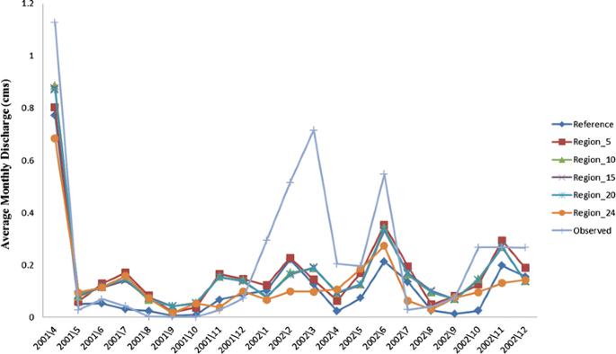
Plot of the comparison between averages of monthly simulated and observed discharge (April 2001–December 2002)
The NSE values for the prediction of surface runoff were 0.60, 0.57, 0.60, 0.59, 0.59, and 0.41, and the R 2 values were 0.72, 0.67, 0.69, 0.69, and 0.63, for the Reference, Region_5, Region_10, Region_15, Region_20, and Region_24, respectively (Table 4). The performance evaluation was quite good for an uncalibrated model. In other words, to increase these indices, we need to adjust some parameters as would be done under sensitivity analysis. The significant underestimation, especially in the period of January–March 2002, has been attributed to the exceptionally unseasonable near-zero and above-zero temperatures (some as high as 10 °C) recorded. SWAT had difficulty in distinguishing between rainfall and snowfall given its weather-generating method (Deslandes et al. 2004; Michaud et al. 2007)
Table 4 The Performance assessment of SWAT configurations using R 2 and the Nash–Sutcliffe coefficient -
Sediment. The time series plot of the simulated and observed sediment load is shown in Fig. 9. A comparison shows that SWAT configurations capture the peak flow periods and also the low flow periods. The NSE was poor, being less than 0.3 in all cases (Table 4). The R 2 was 0.58 in all cases, except for Region_24 for which it was 0.45 (Table 4).
Fig. 9 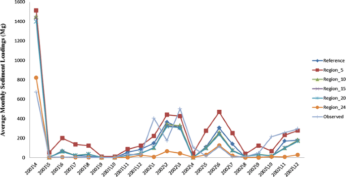
Plot of the comparison between averages of monthly simulated and observed sediment load (April 2001–December 2002)
-
Total phosphorus. The plot of measured vs. uncalibrated TP load predicted is shown in Fig. 10. Although the SWAT configurations captured high fluxes due to high flows, in all cases, it underpredicted the P fluxes. The coefficients of determination were 0.83, 0.78, 0.85, 0.85, and 0.88 for Reference, Region_5, Region_10, Region_15, Region_20, and Region_24, respectively (Table 4).
Fig. 10 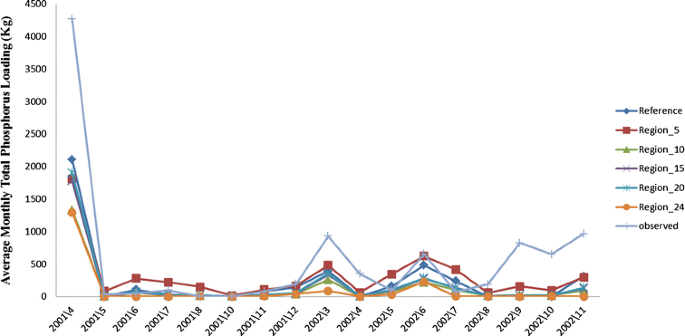
Plot of the comparison between averages of monthly simulated and observed total phosphorus load (April 2001–November 2002)


3.3.3 Sensitivity Analysis
Before calibration, sensitivity analysis is a process that must be performed to know which parameters to adjust during the calibration procedure and by how much. We used the sequential uncertainty fitting (SUFI) version 2 algorithm in SWAT calibration and uncertainty procedures to carry out this process. SUFI is used to derive the posterior parameters from priors. In other words, parameter uncertainty accounts for all sources of uncertainties such as the uncertainties in inputs (such as rainfall), model structure, and observed data (Abbaspour et al. 2007). A 95 % uncertainty is obtained at the 2.5 and 97.5 % levels of the cumulative distribution of the input variable derived by the Latin hypercube sampling (Abbaspour et al. 2007). The parameters shown in Table 5 were found to be the most sensitive for hydrology for all SWAT configurations after 1,000 simulations. The t-stat provides a measure of sensitivity, while the p values determined the significance of the sensitivity (Abbaspour et al. 2007). A value close to zero has more significance (Abbaspour et al. 2007). Therefore, in Table 5, the base flow factor (ALFA_BF), base flow alpha factor for bank storage (ALPHA_BNK), and Manning's “n” value for the main channel (CH_N2) are the most sensitive parameters followed by SCS runoff CN2.
3.3.4 After Calibration for Hydrology, Sediment, and TP
In terms of hydrology, model performance was evaluated using R 2 and NSE. In all cases, R 2 is greater than 0.6, while NSE is up to 0.6 for all configurations except Region_24 (Table 4). As for sediment load, USLE support, biological mixing efficiency, peak rate adjustment factor for sediment routing in the main channel, and peak rate adjustment factor for sediment routing in the sub-basins were the parameters that were adjusted. There were significant improvements in the models' performance based on NSE. The R 2 also increases. For TP, SWAT predictions were hardly improved compared to the uncalibrated results. The following parameters were adjusted, namely phosphorus sorption coefficient, phosphorus percolation coefficient, and phosphorus soil partitioning coefficient. R 2 equally ranges from 0.72 to 0.85 across all configurations.
Generally, the essence of calibration in hydrology is to modify the input parameters to a hydrologic model until the output from the model matches an observed set of data. There are uncertainties in the observed set of data. Also, the conceptualization or structure of the model is not free from uncertainties. Therefore, it is possible to have lower performance indices such as R 2 and NSE after calibration as seen in this study and in other literature (Srinivasan et al. 2010). Also, Mukundan et al. (2010) reported that calibration can mask important parametric information. In fact, Heathman et al. (2008) attested that hydrologic models in uncalibrated mode eliminate bias due to parameter optimization.
Overall, it can be said that all SWAT configurations perform at the same scale compared with the observed data. Putting the reference configuration into perspective, one may not necessarily be losing much information using the average values. In other words, having detailed or high-resolution information, especially for soil properties, does not necessarily improve the prediction in the face of model structural uncertainty. Use of CN in SWAT tends to mask or cover what would have been the impact of different soil properties.
4 Concluding Remarks
The impact of soil heterogeneity in predicting runoff, sediment load, and TP was examined in this study. Five different soil configurations that were partitioned and regionalized to account for heterogeneity at various stages (5, 10, 15, 20, and 24 heterogeneous regions) were investigated. This method showed that when a sample point is a region unto itself, the measure of within-region heterogeneity is lowest. In other words, the greater the number of regions, the lesser the within-region heterogeneity is. From an HRU perspective, there are significant differences in their distributions. However, this does not translate into differences in model prediction.
Results showed that an increase in spatial detail by taking more soil measurements does not necessarily increase the accuracy of the model predictions. The use of curve numbers in SWAT tends to mask any discrepancies because it is based on the soil hydrologic group, which conceals the different physical properties of the soil. This is part of the uncertainty in the model structure that needs to be addressed. Therefore, hydrologists need to weigh the pros and cons of having high-resolution data and the cost involved. As demonstrated in this study, having more samples and using them as individual units without averaging does not necessarily improve the predictions.
References
Abbaspour, K. C., Vejdani, M., & Haghighat, S. (2007). SWAT-564 CUP calibration and uncertainty programs for SWAT. http://www.mssanz.org.au/MODSIM07/papers/24_s17/SWAT-UP_s17_Abbaspour_.pdf. Accessed 02 Feb 2013.
Arnold, J. G., Srinivasan, R., Muttiah, R. S., & Williams, J. R. (1998). Large area hydrologic modeling and assessment—Part I: model development. Journal of the American Water Resources Association, 34(1), 73–89.
Bernassi, F., & Ferrara, R. (2010). Regionalization with dynamically constrained agglomerative clustering and partitioning: an application on spatial segregation of foreign population in Italy at regional level. In 45th Scientific meeting of the Italian statistical society. Padua: University of Padua. 29 July 2010b.
Bowles, J. E. (1986). Engineering properties of soils and their measurement. New York: McGraw-Hill.
Burk, L., & Dalgliesh, N. (2008). Estimating plant available water capacity—a methodology. Canberra: CSIRO Sustainable Ecosystems.
Deslandes, J., Michaud, A., & Bonn, F. (2004). Use of GIS and remote sensing to develop indicators of phosphorus non-point source pollution in the Pike River Basin. In T. O. Manley, P. L. Manley, & T. B. Mihuc (Eds.), Lake Champlain: partnerships and research in the new millennium (pp. 271–290). New York: Kluwer Academic/Plenum Pub.
Deslandes, J., Beaudin, I., Michaud, A., Bonn, F., & Madramootoo, C. A. (2007). Influence of landscape and cropping system on phosphorus mobility within the Pike River watershed of southwestern Quebec: model parameterization and validation. Canadian Water Resources Journal, 32(1), 21–42. doi:10.4296/cwrj3201021.
Donkin, M. J. (1991). Loss-on-ignition as an estimator of soil organic carbon in A-horizons of forestry soils. Communication in Soil Science Plant Analysis, 22, 233–241.
ESRI, (2012). Create Thiessen polygons. http://resources.arcgis.com/en/help/main/10.1/index.html#//00080000001m000000. Accessed 20 December 2012.
Gassman, P. W., Reyes, M. R., Green, C. H., & Arnold, J. G. (2007). The soil and water assessment tool: historical development, applications and future research directions. Transactions of the ASABE, 50(4), 1211–1250.
Guo, D. (2008). Regionalization with dynamically constrained agglomerative clustering and partitioning (REDCAP). International Journal of Geographical Information Science, 22(7), 801–823
Heathman, G. C, Flanagan, D. C., Larose, M., & Zuercher, B. W. (2008). Application of the soil and water assessment tool and annualized agricultural non-point source models in the St. Joseph River watershed. Journal of Soil and Water Conservation. 63(6). doi:10.2489/jswc.63.6.552.
Hegman, W., Wang, D., & Borer, C. (1999). Estimation of Lake Champlain basinwide nonpoint source phosphorus export. Lake Champlain basin program technical report no. 31. Grand Isle: LCBP.
Jamieson, A., Madramootoo, C. A., & Enright, P. (2003). Phosphorus losses in surface and subsurface runoff from a snowmelt event on an agricultural field in Quebec. Canadian Biosystems Engineering, 45(1), 1–7.
MDDEPQ (Ministère du Développement durable, Environnement et Parcs du Quebec MDDEPQ). (2005). Le réseau hydrométrique québécois 1998 à 2003. [Quebec's hydrological network 1998–2003.] MDDEPQ, Centre d’expertise hydrique du Quebec. http://www.cehq.gouv.qc.ca/hydrometrie/reseau/index.htm. Accessed 02 Jan 2013.
MDDEPQ (Ministère du Développement durable, Environnement et Parcs du Quebec). (2003). Base de données Climatologique du Quebec de 1997 à 2003. [Climatological database for Quebec, 1997–2003]. Service de l’information sur le milieu atmosphérique, Direction du suivi de l’état de l’environnement. http://www.hc-sc.gc.ca/ewh-semt/pubs/eval/inventory-repertoire/climatologie_f.html. Accessed 02 Feb 2013.
Medalie, L., & Smeltzer, E. (2004). Status and trends of phosphorus in Lake Champlain and its tributaries, 1990–2000. In T. O. Manley, P. L. Manley, & T. B. Mihuc (Eds.), Lake Champlain: partnerships and research in the new millennium (pp. 191–219). New York: Kluwer Academic/Plenum.
Michaud, A. R. (2004). Indicateurs Agroenvironnementaux Adaptes A la Gestion De Project Cibles Sur la Prévention De la Pollution Diffuse par le Phosphore. Faculté Des Sciences De l’agriculture et De l’alimentation. Québec: Université Lava.
Michaud, A. R., Beaudin, I., Deslandes, J., Bonn, F., & Madramootoo, C. A. (2007). SWAT-predicted influence of different landscape and cropping system alterations on phosphorus mobility within the pike river watershed of southwestern Québec. Canadian Journal of Soil Science, 87(3), 329–344.
Michaud et al. (2008). Beneficial management practices and water quality: hydrological modeling of two basins in the Monteregie region (Quebec). National Agric-Environmental Standards Initiative Technical Series Report No. 4–65. Gatineau: Prepared and published by Environment Canada
Mishra, S. K., & Singh, V. P. (2003). Soil conservation service curve number (SCS-CN) methodology. Dordrecht: Kluwer Academic Publishers.
Mukundan, R., Radcliffe, D. E., & Risse, L. M. (2010). Spatial resolution of soil data and channel erosion effects on SWAT model predictions of flow and sediment. Journal of Soil and Water Conservation. doi:10.2489/jswc.65.2.92.
Nash, J. E., & Sutcliffe, J. V. (1970). River flow forecasting through conceptual models. Part I: a discussion of principles. Journal of Hydrology, 10(3), 282–290.
Neitsch, S. L., Arnold, J. G., Kiniry, J. R., William, J. R., & King, K. W.; Grassland, Soil and Water Research Laboratory of the USDA Agricultural Research Service; Blackland Research and Extension Center (2009). Soil and water assessment tool theoretical documentation. College Station: Texas Water Resources Institute Report TR-191. http://twri.tamu.edu/reports/2011/tr406.pdf. Accessed 02 Feb 2013.
Prasad, R., & Power, F. J. (1997). Soil fertility management for sustainable agriculture. New York: Lewis Publishers.
Somenahally, A., Weindorf, D. C., Darilek, L., Muir, J. P., Wittie, R., Thompson, C., et al. (2009). Spatial variability of soil test phosphorus in manure-amended soils on three dairy farms in North Central Texas. Journal of Soil and Water Conservation, 64(2), 89–97.
Srinivasan, R., Zhang, X., & Arnold, J. (2010). SWAT ungauged: hydrological budget and crop yield predictions in the Upper Mississippi River Basin. Transactions of the ASABE, 53(5), 1533–1546.
Steinman, A. D., & Denning, R. (2005). The role of spatial heterogeneity in the management of freshwater resource. In G. M. Lovett, C. G. Jones, M. G. Turner, & K. C. Weathers (Eds.), Ecosystem function in heterogeneous landscapes (pp. 367–387). New York: Springer.
Tague, C. (2005). Heterogeneity in hydrologic processes: a terrestrial hydrologic modeling perspective. In G. M. Lovett, C. G. Jones, M. G. Turner, & K. C. Weathers (Eds.), Ecosystem function in heterogeneous landscapes (pp. 119–135). New York: Springer.
Wischmeier, W. H., & Smith, D. D. (1978). Predicting rainfall erosion losses—a guide to conservation planning. Washington, DC: U.S. Department of Agriculture (handbook no. 537).
Ye, X. C., Viney, N. R., & Zhang, Q. (2009). Effects of spatial resolution of soil data on hydrological processes modelling: a case study suing the SWAT model. 18th World IMACS/MODISIM Congress, Cairns, Australia 13–17 July, 2009.
Author information
Authors and Affiliations
Corresponding author
Rights and permissions
Open Access This article is distributed under the terms of the Creative Commons Attribution License which permits any use, distribution, and reproduction in any medium, provided the original author(s) and the source are credited.
About this article
Cite this article
Boluwade, A., Madramootoo, C. Modeling the Impacts of Spatial Heterogeneity in the Castor Watershed on Runoff, Sediment, and Phosphorus Loss Using SWAT: I. Impacts of Spatial Variability of Soil Properties. Water Air Soil Pollut 224, 1692 (2013). https://doi.org/10.1007/s11270-013-1692-0
Received:
Accepted:
Published:
DOI: https://doi.org/10.1007/s11270-013-1692-0