Feedback-based resource management for multi-threaded applications

Abstract

Reconciling the constraint of guaranteeing to always meet deadlines with the optimization objective of reducing waste of computing capacity lies at the heart of a large body of research on real-time systems. Most approaches to doing so require the application designer to specify a deeper characterization of the workload (and perhaps extensive profiling of its run-time behavior), which then enables shaping the resource assignment to the application. In practice, such approaches are weak as they load the designer with the heavy duty of a detailed workload characterization. We seek approaches for reducing the waste of computing resources for recurrent real-time workloads in the absence of such additional characterization, by monitoring the minimal information that needs to be observable about the run-time behavior of a real-time system: its response time. We propose two resource control strategies to assign resources: one based on binary-exponential search and the other, on principles of control. Both approaches are compared against the clairvoyant scenario in which the average/typical behavior is known. Via an extensive simulation, we show that both techniques are useful approaches to reducing resource computation while meeting hard deadlines.

1 Introduction

The correctness of the run-time behavior of safety-critical applications needs to be verified prior to their deployment. In the context of computational systems that interact with the physical world and must take action in a timely manner, the correctness is defined not only in terms of functionality but also timing. Timing correctness of such systems is generally specified in terms of guarantees of meeting pre-specified deadlines.

In order to verify timing correctness, system designers model the potential behaviors of the system. To have a high degree of confidence that the conclusions drawn based on analysis of these models will hold for actual run-time behavior, these models are required to be conservative. Provisioning computing resources on the basis of such conservative models tends to lead to significant over-provisioning, and subsequently to very poor platform resource utilization during run-time. The safety-critical systems research community has widely recognized this problem, and a variety of approaches have been proposed for dealing with it such as mixed-criticality analysis (Vestal 2007; Burns and Davis 2017) and probabilistic analysis (Bernat et al. 2002; Cucu-Grosjean et al. 2012) of run-time behavior.

In this paper, we will consider parallel tasks as a scenario to explore another approach for modeling and checking the timing correctness of safety-critical systems. Often, parallel tasks in the real-time literature are represented using complex models such as DAGs—while these representations are accurate and can represent the detailed internal structure of tasks, they are often difficult to generate and expensive to analyze. In addition, for some applications, different runs may generate different dependencies, making it difficult to represent them using a single DAG. In this paper, we will explore measurement-based models where, instead of modeling the full complexity of the program, we will model parallel tasks with a couple of parameters only: the work—the total execution needed to complete the task; and the span—the running time of the task if it is given an infinite number of processors.

Even with this simpler model, the problem of pessimistic modeling remains. To guarantee safety, one might estimate the work and span of the DAG to be very large and these large values may not manifest very often (or indeed, ever) in practice. Therefore, allocating resources based on these estimates leads to over-allocation. Prior work (Agrawal and Baruah 2018) has considered an approach similar to the one undertaken in mixed-criticality systems: instead of modeling the task with just one value each of work and span, it is modeled using both its worst-case parameters and typical case parameters. The requirement is that we must guarantee safety in the worst case. In particular, we are given a task with worst-case work W and worst-case span L which must be completed within D time units (its deadline). However, we might expect that most executions of the task will have a substantially smaller work and span. Therefore, during run-time, one can first start by allocating fewer resources based on the typical case, and then increase resources if the typical case assumptions do not hold.

This research In this work, we develop an approach to conserve resources in the typical case (where the computational requirements of the task are smaller than the worst-case parameters), while still guaranteeing that the task will meet deadlines even if the task does manifest its worst-case execution. Our particular approach is sketched below and exemplified by Fig. 1.

• 1. We assume we have a single periodic or sporadic task that must be scheduled on M processors within D time units of arrival. The worst-case work W and span L parameters of a task are known—no job of the task has a larger work or span than specified by these parameters. Further, we assume that it is feasible to schedule this task on M processors in the worst case.

• 2. However, typically jobs of the task have a smaller work and span—this typical case may not be known or may change over time.

• 3. The scheduler first allocates $m\le {\mathrm{M}}$ processors to the job for $V < D$ time units—the expectation is that most of the time (in the typical case) the job will complete within this time, thereby conserving computing resources.

• 4. If the job does not complete within this time, all processors are allocated for the remaining time $D-V$.

The goal is to compute m and V such that the job completes within its deadline even in the worst case—where it has work as large as W and span as large as L. The values of m and V are related, once we pick one, the other is constrained. There may be many pairs $(m,V)$ which satisfy this criterion—we want to pick the largest V and smallest m such that the jobs complete by time V in the typical case while still completing by time D in the worst case. If the typical case values of work and span are known and remain constant, we can use those to pick appropriate values of m and V. However, these parameters may be unknown and may change over time as the task releases a sequence of jobs. We propose a generalization that does not require additional characterization of run-time behavior (beyond the worst-case characterization that is needed to assure safety). Our generalized approach is based on monitoring past executions and making resource-allocation decisions based on the information that is obtained via such monitoring. We explore different techniques, drawn from the sub-disciplines of control theory and algorithm design, for making such resource-allocation decisions.

Fig. 1

The parallel task begins execution at time-instant 0 with a deadline at time-instant D. It executes upon m processors over the interval $[0,{V})$, and upon M processors over the interval $[{V},D)$. (The x-axis thus denotes time, and the y-axis, the number of assigned processors)

Contributions and Organization This paper makes the following contributions:

• 1. Section 3 provides a general strategy for calculating m and V—in particular, given an instantiation of one parameter, how we can safely set the other parameter while guaranteeing safety. In Sect. 4 we instantiate this scheduling strategy to situations in which some additional information, viz. the typical case values of the parameters characterizing the parallel tasks, are known. These sections are a simplified restatement of work from Agrawal et al. (2020).

• 2. In Sect. 5, we derive, and prove correct, algorithms for scheduling such tasks in the general situation where these typical-case parameters are not known, and furthermore when these typical-case values may vary over time. In this section, we explore two general strategies, one based on binary-exponential search, and one based on proportional control algorithms. Both these strategies observe the behavior of the task over time and continually change the settings of m and V to maximize utilization of the system.

• 3. In Sect. 6, we evaluate the effectiveness of our proposed algorithms via a wide range of simulation experiments on synthetically-generated workloads. These experiments indicate that both our algorithms perform well, but have different characteristics. The binary-exponential algorithm converges quickly but has a larger variation compared to the control-based algorithm.

In addition to the above section, Sect. 2 explains the model and its motivations, we briefly review the related work in Sect. 7 and conclude in Sect. 8 by placing this work within a larger context of the resource-efficient implementation of hard real-time systems.

2 Measurement-based modeling and scheduling of parallel tasks

In this section, we flesh out the details of a measurement-based model for representing parallel tasks and describe a general strategy for scheduling tasks that are modeled in this manner. We will first motivate the model informally in Sects. 2.1 and 2.1. Then, a formal definition of the model is provided in Sect. 2.3.

2.1 Motivation: revising existing models

As stated in Sect. 1, several excellent DAG-based models for representing parallel real-time code have been developed in the real-time community; however, there are some classes of real-time applications for which such models have proved unsuitable. This may be for one or more of the following reasons:

• 1. The internal structure of the parallel code may be very complex, with multiple conditional dependencies (as may be represented in e.g., the conditional DAG tasks model (Melani et al. 2015; Baruah et al. 2015) and (bounded) loops. Explicit enumeration of all possible paths through such code in order to identify worst-case behavior may be computationally infeasible.¹

• 2. If some parts of the code are procured from outside the application developers’ organization, the provider of this code may seek to protect their intellectual property (IP) by not revealing the internal structure of the code and instead only providing executables—this may be the case if, e.g., commercial vision algorithms are used in a real-time application.

• 3. Explicitly representing the internal structure of the DAG generated by some code can be exponential in the size of the code. In addition, algorithms for the analysis of systems represented using DAG-based models tend to have run-time pseudo-polynomial or exponential in the size of the DAG. Therefore, in aggregate, these runtimes may become too large to be useful in practice.

• 4. Particularly for conditional code, it may be the case that the true worst-case behavior of the code is very infrequently expressed during run-time.

For pieces of parallel real-time code possessing one or more of the characteristics discussed above, DAG-based representations may not be appropriate for schedulability analysis; alternative representations are needed. Let us now discuss what such a representation should provide.

2.2 Approach: Identifying relevant characteristics of parallelizable real-time code

In modeling parallelizable real-time code that is to be executed upon a multiprocessor platform, a prime objective is to enable the exploitation of the parallelism that may be present in the code by scheduling algorithms, to enhance the likelihood that we will be able to meet timing constraints. We are interested here in developing predictable real-time systems—systems that can have their timing (and other) correctness verified prior to run-time. To enable a priori timing verification, decades of research in the parallel computing community suggest the following two timing parameters of a piece of parallelizable code are particularly significant:

• 1. The work parameter W denotes the cumulative worst-case execution time of all the parallel branches that are executed across all processors. Note that for non-conditional parallelizable code this is equal to the worst-case execution time of the code on a single processor (ignoring communication overhead from synchronizing processors).

• 2. The span parameter L (also called the critical path length in the literature) denotes the maximum cumulative worst-case execution time of any sequence of precedence-constrained pieces of code. The total running time of the program on any number of processors is at least equal to its span.

The relevance of these two parameters arises from well-known results in scheduling theory. While scheduling a DAG to minimize its completion time is NP-hard in the strong sense, Graham’s list scheduling algorithm (Graham 1969), which constructs a work-conserving schedule by executing at each instant in time an available job upon any available processor, performs fairly well in practice. In particular, it has been proved in Graham (1969) that the response time R of the DAG, which is the time elapsing from the release to the completion of the DAG, is guaranteed to be no larger than

$$\begin{aligned} R \le \frac{W- L}{{\mathrm{M}}} + L\end{aligned}$$

(1)

when the DAG is scheduled over M machines. The analogous term makespan is often used in the scheduling community.

A little thought makes it clear that this bound is $(2-\frac{1}{{\mathrm{M}}})$-competitive—no scheduler can finish the job in less than $R/(2-\frac{1}{{\mathrm{M}}})$ time – suggesting that list scheduling is a reasonable algorithm to use in practice. In fact, most run-time scheduling algorithms for DAGs upon multiprocessors use different flavors of list scheduling.

2.3 Formal system model

We now provide a formal definition of our model, by describing in detail our workload model. A parallel task is characterized by

• W is a conservative estimate of the total computational requirement of the job over all the processors (the work),

• L is the conservative estimate on the longest path of dependencies in the task (the span) and

• D denotes the relative deadline parameter: a correct execution requires that the response time upper bound of (1) is no greater than D that is

  $$\begin{aligned} \frac{W- L}{{\mathrm{M}}} + L\le D \end{aligned}$$

  (2)

In this paper, we consider the scheduling of a single such task upon a dedicated bank of identical processors. We point out that our results are directly applicable to the scheduling of multiple recurrent—periodic or sporadic—real-time DAGs where each instantiation of the task is called a job. We assume that we have a multiprocessor or a multicore where each task is assigned a set of dedicated processors for execution and need not worry about the other tasks running on the same machine. Here, we assume that each periodic/sporadic task satisfies the additional constraint that its relative deadline parameter is no larger than its period parameter (i.e., they are constrained-deadline tasks).

We assume that timing correctness is specified assuming that W and L are correct estimates: the code is required to complete execution within the specified relative deadline D provided its work and span parameters are no larger than W and L respectively.

Fig. 2

Illustrating the notions of worst-case work and span. Numbers in vertices represent the required processing time of the vertex, while arrows denote precedence between vertices. The figure shows five possible realizations of a DAG with worst-case work and span respectively equal to equal to $W=20$ and $L=12$. We observe that the general notions of work and span generalize DAGs with very different dependencies, possibly even fully independent vertices (fourth case) or just sequential work (fifth case). The only requisite is that the work and span of the realization do not exceed the worst-case values

Note that the work and span parameters are not, in themselves, fully descriptive of the program itself. Consider the examples in Fig. 2. The work and span $(W,L)$ of the individual DAGs in these figures are (20, 12), (20, 10), (20, 12), (20, 6), (12, 12) respectively. However, a particular task may generate many different DAGs varying from instance to instance. If we had a program that could generate all these jobs, then we would define the worst-case work and span as defined in our model as 20 and 12, respectively. In particular, even if the program could only generate the last two DAGs, we would still define the worst-case work as 20 and the worst-case span as 12 even though no individual instantiation of the program can simultaneously have work of 20 and the span of 12.

3 Sufficient schedulability conditions

As described in Sect. 1 and illustrated in Fig. 1, given a task modeled by the parameters (W, L, D) as described above that is to be implemented upon an M-processor platform, we want to compute m and V such that we can both (i) guarantee safety and (ii) improve performance in the typical case. In this section, we will compute the sufficient schedulability conditions which guarantee safety. In particular, we will derive the relationship between m and V such that any values that satisfy this relationship can ensure that the job will complete by its deadline. In later sections, we will use this condition to calculate specific values that can be used to get good performance in the typical case.

Suppose that we are given values of m and V (with $0< m\le {\mathrm{M}}$ and $0\le {V} \le D$), and the run-time algorithm schedules the task on m processors using list scheduling. If the task completes execution within V time units, correctness is preserved since ${V}\le D$. It remains to determine sufficient conditions for correctness when the task does not complete by time-instant V.

Figure 1 depicts the processors that are available for this task if it does not complete execution within V time units, thereby resulting in the run-time scheduler allocating the additional $({\mathrm{M}}-m)$ processors. (These processors may have been allocated to other, non real-time work over the period $[0,{V})$ or they may be put to sleep to conserve energy). We will now derive conditions for ensuring that the task completes execution by its deadline at time-instant D when executing upon these available processors, given that its work parameter may be as large as W and its span parameter, L.

Let $W^{\prime}$ and $L^{\prime}$ denote the work and span parameters of the amount of computation of the parallel task that remains at time-instant V (these are strictly positive quantities since the task is assumed to not have completed execution by time-instant V). This remaining computation executes upon M processors. By Eq. (1) the response time R of the DAG is upper bounded by

$$\begin{aligned} R\le {V}+ \left( \frac{W^{\prime}-L^{\prime}}{{\mathrm{M}}} + L^{\prime} \right) \end{aligned}$$

(3)

Consider the time period until V in this execution and say that there were X time steps where all m processors were busy and Y time steps where not all processors are busy. Since the remaining span reduces on each time step when all processors are not busy (and may reduce on the other time steps as well), we have $L- L^{\prime} \ge Y$. Therefore, $X = {V}-Y \ge {V}- (L- L^{\prime})$. Hence the total amount of execution occurring over $[0,{V})$ is at least

$$\begin{aligned} X m\ge \Bigl ({V}- (L-L^{\prime})\Bigr )\, m, \end{aligned}$$

from which it follows that

$$\begin{aligned} W^{\prime} &\le W- {V}\, m+ (L-L^{\prime})\, m \end{aligned}$$

(4)

Substituting Inequality (4) into (3), the response time upper bound becomes equal to:

$$\begin{aligned}&{V}+ \left( \frac{ W- {V}\, m+ L\, m- L^{\prime}\, m-L^{\prime}}{{\mathrm{M}}} + L^{\prime} \right) \\ &\quad ={V}+ \Bigl (\frac{ W- {V}\, m+ L\, m}{{\mathrm{M}}} + L^{\prime}\, \bigl (1 - \frac{m+1}{{\mathrm{M}}}\bigr )\Bigr ) \end{aligned}$$

(5)

Since $m\le {\mathrm{M}}$, the upper bound of (5) is maximized when $L^{\prime}$ is large as possible; i.e., $L^{\prime} = L$ (the physical interpretation is that the entire critical path executes after V). Substituting $L^{\prime}\leftarrow L$ into Expression (5), we get the following upper bound on the response time:

$$\begin{aligned} {{V}+ \Bigl (\frac{ W- {V}\, m+ L\, m}{{\mathrm{M}}} + L\, \bigl (1 - \frac{m+1}{{\mathrm{M}}}\bigr )\Bigr )}\\ = {V}+ \bigl (\frac{ W- {V}\, m- L}{{\mathrm{M}}} + L\bigr ) \end{aligned}$$

Correctness is guaranteed by having the response time bound be $\le D$, that is:

$$\begin{aligned}&\Bigl ({V}+ \bigl (\frac{ W- {V}\, m- L}{{\mathrm{M}}} + L\bigr )\Bigr ) \le D \\ & \Leftrightarrow \Bigl ({V}- \frac{{V}\, m}{{\mathrm{M}}} \Bigr )\le \Bigl (D - \frac{W-L}{{\mathrm{M}}} - L\Bigr ) \\ & \Leftrightarrow {V}\Bigl (1- \frac{m}{{\mathrm{M}}} \Bigr )\le \Bigl (D - \frac{W-L}{{\mathrm{M}}} - L\Bigr ) \end{aligned}$$

(6)

The condition of (6) is thus the sufficient schedulability condition we seek: values of m and V satisfying (6) guarantee correctness.

4 Resource allocation when typical parameter values are known

In this section, we will assume that we have some additional prior information—namely, we know typical or nominal values of the work and span parameters—$W_{\scriptscriptstyle T}$ and $L_{\scriptscriptstyle T}$. These parameters bound the work and span values of a “typical” invocation of the task and are derived via measurements or more optimistic analysis techniques. For the remainder of this section only, the expectation is that these values exist and are known. Later in Sect. 5, we will consider the case where the DAG does not exhibit any typical behavior. It will be then our proposed logic that infers the values that are to be assigned to the $W_{\scriptscriptstyle T}$ and $L_{\scriptscriptstyle T}$ parameters.

We saw in Sect. 3 that choosing the parameters m and V satisfying the condition of (6) ensures the correctness of the scheduling algorithm. We will use the nominal parameters to pick a particular pair of values from this space. Our goal here is efficiency: we want to use the minimum amount of computational resources under the typical circumstances. Therefore, we want to minimize the product of m and V.

By Inequality (1), we know that upon m processors a typical invocation (an execution with work and span bounded by $W_{\scriptscriptstyle T}$ and $L_{\scriptscriptstyle T}$ respectively, will complete no later than $\bigl ((W_{\scriptscriptstyle T}- L_{\scriptscriptstyle T})/m+ L_{\scriptscriptstyle T}\bigr )$. Hence, the assignment of

$$\begin{aligned} {V}\leftarrow \Bigl ( \frac{W_{\scriptscriptstyle T}-L_{\scriptscriptstyle T}}{m} + L_{\scriptscriptstyle T}\Bigr ) \end{aligned}$$

(7)

guarantees that if the DAG work and span do not exceed the typical values $W_{\scriptscriptstyle T}$ and $L_{\scriptscriptstyle T}$, respectively, only m cores are used and processing capacity is saved.

Equation 7 makes it clear that the two parameters in the product $m{V}$ have an inverse relationship—as m decreases, V increases. However, we can also see that due to the additive $L_{\scriptscriptstyle T}$ in the equation, we want to pick the minimum feasible m to minimize the product. Recall that we must pick these values to satisfy Eq. (6) to guarantee feasibility in the worst-case—therefore substituting this value V, we get

$$\begin{aligned} \Bigl ( \frac{W_{\scriptscriptstyle T}-L_{\scriptscriptstyle T}}{m} + L_{\scriptscriptstyle T}\Bigr )\, \Bigl (1- \frac{m}{{\mathrm{M}}} \Bigr )\le \Bigl (D - \frac{W-L}{{\mathrm{M}}} - L\Bigr ) \end{aligned}$$

(8)

as a sufficient schedulability condition, which is equivalent to

$$\begin{aligned} a\, m^2 + b\, m+ c \ge 0 \end{aligned}$$

with a, b, and c assigned the following values:

$$\begin{aligned} a & \leftarrow L_{\scriptscriptstyle T}\\ b & \leftarrow {\mathrm{M}}\bigl (D - (L+L_{\scriptscriptstyle T}) \bigr ) - (W-L) + (W_{\scriptscriptstyle T}-L_{\scriptscriptstyle T})\\ c & \leftarrow -{\mathrm{M}}\, (W_{\scriptscriptstyle T}-L_{\scriptscriptstyle T}) \end{aligned}$$

By finding the positive root of this second-degree polynomial, we find that the number of cores m assigned over [0, V] should be

$$\begin{aligned} m\leftarrow \left\lceil \frac{-b + \sqrt{b^2 - 4\,a\,c}}{2\,a} \right\rceil \end{aligned}$$

(9)

and the corresponding value of V is set by Eq. (7). Algorithm 1 reports the pseudo-code for assigning both m and V.

4.1 Run-time complexity

Algorithm 1 comprises straight-line code with no loops or recursive calls. Hence, given as input the parameters specifying a task, it is evident that Algorithm 1 has constant—$\Theta (1)$—run-time.

In the rest of the paper, the typical parameters are assumed to be unknown. We will be using the typical parameters of the DAG as an oracle to compare approaches that ignore this additional information. Therefore, we will use $m_{\mathsf{id}}$ to refer to the ideal allocation of cores of (9), which is aware of the typical parameters $W_{\scriptscriptstyle T},L_{\scriptscriptstyle T}.$

5 Observation-based adaptation of resource allocation decisions

In the previous section, we had assumed that the typical work and span values were known a priori and that these values remain constant as the system continues to execute. Under these assumptions, we were able to compute the optimal allocation of $(m,{V})$. A resource allocation scheme relying on “typical” parameters, however, may be very inefficient because typical parameters may not exist due to the uncertain and variable nature of DAG workloads. In the following we investigate runtime observation-based mechanisms to adapt the allocation of $(m,{V})$ over multiple iterations, relaxing such assumptions.

5.1 Response-time based processor allocation

We now describe the general scheme for optimizing resources assigned to recurrent applications, while maintaining the guarantee that the application always meets its deadline. Figure 3 illustrates the general scheme and the equations of the dynamics of our monitoring-based decision-making process for controlling the allocation of resources to an application modeled as a recurrent multi-threaded application. Similar feedback-based schemes can be found also in the cloud computing literature literature (Lorido-Botran et al. 2014; Jennings and Stadler 2015; Papadopoulos et al. 2016), where different autoscaling techniques have been proposed. However, autoscaling techniques are usually not concerned with (hard) real-time guarantees, and they are more focused on developing techniques for workload prediction to perform prompt and proactive scaling.

Fig. 3

A general diagram for the decision-making process and the corresponding dynamics

In the equations in Fig. 3, we use the following terms

• $\mathsf{state}(k)$ is the internal state of the decision-making algorithm at the k’th iteration

• $\mathsf{runtime}(k)$ is the monitored run-time measurements

• $\mathsf{resource}(k)$ is the resource allocation at the k’th iteration

• $\mathsf{nextState}(\dots )$ describes the internal logic of the decision-making algorithm (in the following, three different algorithms are proposed)

• $\mathsf{resourceAlloc}(\dots )$ determines the resource allocation for a given state of the decision-making algorithm.

The above description is quite general. There are many possible run-time measurements and many different types of resources to be controlled. In this paper, our goal is to design a simple resource allocation scheme enabled by minimal monitoring in order to demonstrate the applicability of the general idea.

One could envision monitoring different aspects of the run-time behavior modeled by $\mathsf{runtime}(k)$, for example

• the response time of the DAG;

• the total amount of computing capacity consumed by the DAG;

• the progress of the DAG execution along different paths, possibly monitored by instrumenting the DAG code.

These are all reasonable solutions, and each offers a different level of detail. As a general principle, the richer the monitored information is, the more efficient any resource allocation decisions can be. Acquiring richer (and more fine-grained) information may, however, require greater effort on the part of the system developer, or may not even be possible via the available interfaces. In addition, monitoring itself typically adds overheads and disturbs the system—therefore, heavyweight monitoring may provide additional information for too high a cost.

In this work, we make the following assumption of minimal monitoring.

Assumption 1

The only information detected by run-time monitoring is the response time R of each job.

This assumption makes our approach very general, and applicable in a broad variety of settings. Using the formalism introduced above, this assumption means that

$$\begin{aligned} \mathsf{runtime}(k) = R(k), \end{aligned}$$

where R(k) denotes the response time of the kth job—the kth invocation of the DAG task.

In addition, the amount of computing resources $\mathsf{resource}(k)$ allocated to schedule the DAG during an invocation may be set in several different ways. Examples include:

• The number of processors/cores allocated;

• The frequency at which subsets of the cores are run;

• The fraction of computing capacity allocated (via resource reservation schemes); and

• Various combinations of the above methods.

Again, as we privilege simplicity and generality, we make the following assumption regarding resource allocation.

Assumption 2

The computing capacity allocated to the DAG is controlled by setting the number m of cores assigned over the interval $[0,{V})$ at every DAG release, in accordance to the scheduling strategy of Sect. 3.

We note that many OSes do in fact give the user the ability to specify the number of cores of a multi-core platform to assign to individual multi-threaded applications. E.g., one way of doing this on the command line in Linux is by the taskset command or by using the sched_setaffinity(...) system call. Neither method requires superuser privileges.

In this context, the choice of the number of cores m implies the value of the virtual deadline V. In fact, solving the Inequality (6) for V, we obtain that

$$\begin{aligned} {V}\le \frac{{\mathrm{M}}(D-L) - (W- L)}{{\mathrm{M}}-m} \end{aligned}$$

(10)

showing that the choice is coupled, as m upper bounds the choice of V. Moreover, as the main objective of the approach is to minimize the amount of allocated resource for the largest period of time, in the following we will assume that Inequality (10) will hold with the equal sign, and it will be indicated in the following as V(m)—see Eq. (12). In such a way, the only decision variable is m, and the virtual deadline V(m) is a direct function of m. In summary, our proposed resource allocation scheme labeled $\mathsf {resource}(k)$, can be modeled by

$$\begin{aligned} \mathsf {resource}(k) = m(k), \end{aligned}$$

(11)

here $m(k)$ denotes the number of processors initially allocated to the k’th job, and ${V}(m(k))$ is determined by $m(k)$ via Eq. (12).

Remark 1

The virtual deadline ${V} (m)$ is a non-decreasing function of m.

Proof

For $m< {\mathrm{M}}$, the virtual deadline is computed as:

$$\begin{aligned} {V} (m) = \frac{{\mathrm{M}}(D-L) - (W- L)}{{\mathrm{M}}-m} \end{aligned}$$

(12)

Computing the derivative of V with respect to m, we get

$$\begin{aligned} \dfrac{{\text{d}} {V} (m)}{{\text{d}} m} = \dfrac{{\mathrm{M}}(D-L) - (W- L)}{({\mathrm{M}}-m)^2} \end{aligned}$$

and then

$$\begin{aligned} \dfrac{{\text{d}} {V} (m)}{{\text{d}} m} \ge 0 \qquad \Leftrightarrow \qquad {\mathrm{M}}\ge \frac{W- L}{D-L} \end{aligned}$$

which is true due to the schedulability condition of (2). $\square$

Finally, we assume that the assignment of a larger amount of processing capacity leads to a reduction of the response time.

Assumption 3

If $m< m_{\mathsf{id}}$ cores are allocated, then the completion time will exceed the virtual deadline, i.e., $R > {V} (m)$. If $m\ge m_{\mathsf{id}}$, then the completion time will be below the virtual deadline, i.e., $R \le {V} (m)$, and the completion time is a non-increasing function of the number of assigned cores.

We note that, theoretically, this assumption holds for carefully designed versions of list scheduling (Graham 1969) on preemptive processors. It also holds in practice for most compute-bound programs, though it may not hold for memory-bound applications due to locality, cache, and memory bandwidth issues. For the purposes of this paper, we make this assumption and argue that our strategies can be reasonably expected to reduce resource waste. The correctness guarantee (the fact that we will meet deadlines) does not depend on this assumption.

5.2 Unknown and constant typical workload

In this section, we assume that although the values of the typical work and span parameters, $W_{\scriptscriptstyle T}$ and $L_{\scriptscriptstyle T}$, are not necessarily known to the run-time algorithm that is responsible for allocating computing resources, these values do exist and are constant over time. We use a relatively simple binary search method to calculate $m(k+1)$ given the values of $m(k)$ and R(k), which is sketched in Algorithm 2. Note that the algorithm is repeated at every time k with the new measurement R(k). As internal state, the algorithm maintains two values

$$\begin{aligned} \mathsf {state}(k) = \big (lo(k),hi(k)\big ), \end{aligned}$$

where ${\mathrm{lo}}(k) < hi(k)$ for all k and these are initialized to 0 and m, respectively. The algorithm tries to converge to the ideal number of processors $m= m_{\mathsf{id}}$ by doing a binary search between ${\mathrm{lo}}(k)$ and ${\mathrm{hi}}(k)$ and by changing the corresponding values of ${\mathrm{lo}}(k)$ and ${\mathrm{hi}}(k)$ after each iteration. For any job k, we always assign

$$\begin{aligned} m(k) = \left\lceil \frac{{\mathrm{lo}}(k)+{\mathrm{hi}}(k)}{2}\right\rceil , \end{aligned}$$

which corresponds to the function $\mathsf {resourceAlloc}\big (\mathsf {state}(k)\big )$ in the generic skeleton of resource management scheme of Fig. 3.

Lemma 1

The binary search algorithm converges.

Proof

The invariant we maintain is that $lo(k) < m_{\mathsf{id}}\le hi(k)$ in all iterations. This is clearly true in the beginning since we set ${\mathrm{lo}}= 0$ and ${\mathrm{hi}}= M$. Recall Assumption 3 where we know that if $R(k) > {V} (k)$, then $m(k) < m_{\mathsf{id}}$. In this case, we can safely increase increase ${\mathrm{lo}}(k+1)$ to $m(k)$. Similarly, if $R(k) \le {V} (k)$, we know that $m(k) \ge m_{\mathsf{id}}(k)$. Therefore, we can safely set ${\mathrm{hi}}(k+1) = m(k)$.

As in the usual binary search, in each iteration (until convergence), either the ${\mathrm{hi}}$ value reduces or the ${\mathrm{lo}}$ value increases. Therefore, the algorithm will converge when ${\mathrm{lo}}= {\mathrm{hi}}-1$. At this time, $m= {\mathrm{hi}}$ and will not change further. $\square$

5.3 Unknown and time-varying workload

In Sect. 5.2 above we had assumed that the values of $W_{\scriptscriptstyle T}$ and $L_{\scriptscriptstyle T}$, although unknown, remain constant. We now consider a further generalization: the values of $W_{\scriptscriptstyle T}$ and $L_{\scriptscriptstyle T}$ may change over time. We propose two mechanisms to deal with such an unknown and time-varying DAG workload. The first (Sect. 5.3.1) is based on binary-exponential search (Bentley and Yao 1976) and extends the previously described binary search algorithm. The second (Sect. 5.3.2) is a control-based approach.

5.3.1 Binary-exponential search

We now consider the situation where the underlying computation may change from one job to the next. In particular, consider the case where the binary search has converged such that ${\mathrm{lo}}(k)+1 = m(k) = hi(k)$ and then the underlying computation changes so that $R(k) > {V} (k)$. Now we clearly need more processors and the current ${\mathrm{hi}}(k)$ is no longer the correct upper bound on the number of processors we need. Therefore, we must increase ${\mathrm{hi}}(k+1)$. Here we use the idea behind exponential search (Bentley and Yao 1976). We increase ${\mathrm{hi}}(k+1)$ by a small increment (say ${\mathrm{hi}}(k+1) = {\mathrm{hi}}(k) + 2$) to begin with. This causes a small increase in $m(k+1)$. If we still have too few processors, we further increase ${\mathrm{hi}}(k)$, this time by 4, doubling the increase with each iteration until we reach the point where we have a sufficiently large upper bound. At this point, again ${\mathrm{lo}}(k)$ and ${\mathrm{hi}}(k)$ are good upper and lower bounds and the normal binary search allows us to converge. In Algorithm 3, line 3 shows the condition under which we increase ${\mathrm{hi}}(k+1)$. While this condition is correct, it may misfire and may increase ${\mathrm{hi}}$ even when it need not do so—for instance, it may be the case that $m(k) < {\mathrm{hi}}(k)$—therefore, R(k) which is the response time with $m(k)$ processors is larger than ${V} ({\mathrm{hi}}(k))$, but the response time with ${\mathrm{hi}}(k)$ processors (which may be smaller) would not exceed ${V} ({\mathrm{hi}}(k))$ and therefore ${\mathrm{hi}}(k)$ is a good upper bound and need not be increased. In our actual code, we use a slightly better condition which is less likely to misfire. However, this problem can not be perfectly solved since we can not precisely know the response time with ${\mathrm{hi}}(k)$ processors. This problem is related to the observability problem described in the previous section, albeit it is not identical.

A similar exponential change must be made to ${\mathrm{lo}}$ when the response time of the underlying computation decreases. However, this is even more treacherous. Imagine that we have converged to ${\mathrm{lo}}(k)+1 = m(k) = {\mathrm{hi}}(k)$ and we observe that $R(k) < {V} (k)$. By symmetry from the above argument, one would imagine that we should decrease ${\mathrm{lo}}(k+1)$ to decrease $m(k+1)$. However, recall that we want to compute the smallest $m(k+1)$ such that the response time $R(k+1)$ is at most $V(m(k+1))$. Since R(k) may not (in fact, it is unlikely to) exactly equal a virtual deadline corresponding to any particular number of processors, R(k) is generally likely to be smaller than ${V} (m(k))$ even when we have the correct number of processors. Therefore, if we always decrease m when $R(k) < {V} (k)$, the number of processors assigned will oscillate between the “correct value” (where $R < {V}$) and one fewer processor (where $R > {V}$). Therefore, we shouldn’t necessarily decrease the number of processors if the virtual deadline is larger than the response time. To prevent this, on Line 9, we first check if $R(k)<{V} (m(k)-1)$. If R(k) is between ${V} (m-1)$ and ${V} (m)$, then we can be sure that m was the correct allocation and we needn’t decrease ${\mathrm{lo}}(k+1).$

This does not completely solve the problem, however. In particular, in some cases, it is possible that the response time $R(m) < {V} (m-1)$ while $R(m-1)> {V} (m-1)$. In this case, the correct allocation is m. However, with a single observation, no algorithm can distinguish this case from the case where $R(m-1)> {V} (m-1)$. Therefore, for such computations, our algorithm does oscillate between m and $m-1$. It is important to note that this oscillation can not be prevented when we make a single response time measurement. Furthermore, this oscillation automatically solves the observability problem described in Sect. 5.4. In particular, say that $R(k) > {V} (m(k)-1)$. In this case, we can be sure that the response time with $m(k)-1$ processors (which we did not observe) will also be larger than ${V} (m(k)-1)$ due to the non-decreasing property of response time. Therefore, it is not necessary to check with one fewer processor. On the other hand, if the response time $R(k) > {V} (m(k)-1)$, then this algorithm will automatically decrease ${\mathrm{lo}}(k+1)$ and therefore, decrease $m(k+1)$ compared to $m(k)$. As mentioned in Sect. 5.4, this measurement is enough to check if we are using resources inefficiently and if so, the algorithm will converge to a smaller allocation.

5.3.2 Integral controller

A natural choice to explore for the decision-making problem is a control-based approach. Control theory has been extensively used in different domains for runtime adaptation.

The main challenges in applying a control-based solution in this context are:

• 1. The difficulty in determining a model of the system to be controlled. The relation between the amount of allocated resource (“$\mathsf {resource}(k)$” in Fig. 3) and the runtime behavior (“$\mathsf {runtime}(k)$” in Fig. 3) may be unknown or depend on unknown/unavailable internal state (e.g. cache content)

• 2. The definition of an appropriate set point in terms of resource allocation to be reached, and

• 3. The presence of integer variables, while normally feedback control loops work better with real-valued variables.

All three problems are intertwined and need to be addressed jointly.

In a typical control structure, the set point is a well-defined concept that is the desired behavior of the system. In this specific application, the ideal resource allocation $m_{\mathsf{id}}$ is unknown as it depends on the unknown relationship between the resource allocation and the runtime behavior. Therefore, computing such quantity would require knowing exactly the function $R(m)$ for all the possible values of m and for all the time instants—since such function can also vary over time. The control problem can be then formulated as an approximation of the described problem, by measuring the response time of the previous run $R(m(k-1))$, and computing the approximated desired value of cores at the current time instant as:

$$\begin{aligned} m^{sp}(k) := {\mathrm{arg\,min}}_{i} {V} (i) \ge R(m(k-1)) \end{aligned}$$

(13)

(Here, the superscript “sp” denotes “set point.”) If this is applied in an iterative way over time, $R(m(k-1))$ is the result of the allocation $m(k-1)$, $R(m(k))$ is the result of the allocation $m(k)$, and so on.

Recall that Remark 1 states that the virtual deadline ${V}$ is a non-decreasing function of m and that Assumption 3 states that the response time R decreases with increasing values of m when $R \le {V}$. Therefore, if the allocation of $m(k)$ is too low, the resulting response time will be $R(k)>{V}$, and the controller will increase m. On the other hand, if $R(k)\le {V}$ the controller will try to make the two quantities as close as possible, and it will decrease m.

The control strategy can be defined as follows. The tracking error e can be defined as the discrepancy between $m^{sp}(k)$ and the old core allocation as:

$$\begin{aligned} e(k) = m^{sp}(k) - m(k-1) \end{aligned}$$

(14)

The smooth adaptation, can be achieved with an integral control structure:

$$\begin{aligned} \tilde{m}(k) = \tilde{m}(k-1) + K e(k) \end{aligned}$$

(15)

where $K \in (0,1]$, and the symbol $\tilde{m}(k)$ is used to indicate the non-integer number of cores. The resulting number of cores must be saturated between a minimum and maximum value as

$$\begin{aligned} \tilde{m}(k) = \min (\max (\tilde{m}(k),1),{\mathrm{M}}) \end{aligned}$$

(16)

Furthermore, whereas the tracking error e(k) is generally an integer, the resulting number of cores is not necessarily an integer due to the multiplication by the real constant K. The actual number of cores is therefore rounded:

$$\begin{aligned} m(k) = {\mathrm{round}}(\tilde{m}(k)). \end{aligned}$$

(17)

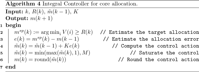
Summarizing, the internal state of the control logic is $\mathsf {state}(k) =\tilde{m}(k)$, while the $\mathsf {nextState}(\cdot ,\cdot )$ function is the composition of Eqs. (14)–(16), and the $\mathsf {resourceAlloc}(\cdot )$ is (17).

The resulting control formulation is presented in Algorithm 4. The formulation has the following advantages:

• 1. it provides a guarantee that the control strategy has a stable attractor in $e(\cdot ) = 0$, meaning that it guarantees convergence either to zero tracking error or to a stable limit cycle around $e(\cdot ) = 0$;

• 2. in the case that the required number of cores is exceeding the saturation values, Eq. (16) avoids the accumulation of the error and then it allows a prompt reaction as soon as the required number of cores becomes again within the saturation limits (the so-called windup effect Åström and Murray 2021); and

• 3. having selected the real-valued number of cores $\tilde{m}$ as the state of the controller, it accumulates the quantity Ke(k) over multiple iterations, causing the computed number of cores $\tilde{m}$ to smoothly change and eventually cross the threshold for the rounding. This enables the exploration of a different number of cores, which may be needed to possibly infer information about the resource usage, not directly available from the monitoring of the response time only (as previously illustrated in Sect. 5.4).

  

5.4 Limits of response-time-based resource allocation

As explained above, the response time is perhaps the simplest and most easily monitored aspect of run-time execution. Using this aspect as the sole basis for resource allocation, however, poses some challenges. This potential issue is illustrated by an example in Fig. 4.

Fig. 4

Example of DAG schedule over 4 and 3 cores. The processing time labeled by “XY” represents the schedule of the “X” vertex of the “Y” job released by the DAG. In the schedule over 4 cores, it can be observed that different processing times of vertices may lead to different amounts of wasted resources. Such a difference, however, cannot be detected by response time which has the same value of $R(1)=R(2)=R(3)=4$ for all three jobs

Let us assume that we have a DAG composed of the six vertices labeled A, B, C, D, E, and F. The precedence constraints among these six vertices are illustrated in Fig. 4 (on the left). In this example, the completion of A enables the execution of B, C, D, and E. The last vertex F may execute only after the preceding vertices B, C, D, and E complete. Two scenarios are considered: the execution of the DAG workload upon 4 cores (upper schedule) and the execution of the same workload upon 3 cores (lower schedule). In both scenarios, the DAG releases three jobs at instants 0, 7, and 14 (the job releases are represented by thick arrows pointing up). The variability of the execution times of each vertex is represented by different durations of each vertex among the three jobs shown in the schedules. The two scenarios show the schedules over 4 and 3 cores respectively of the same three jobs with the same duration of the vertex execution time.

This example shows the implication and the potential issues of using only the response time to allocate the “right” amount of processing resources. When the three jobs of the example are scheduled upon 4 cores, the response times R(1), R(2), and R(3) of the three jobs are all equal to 4. Hence, any resource allocation policy which uses the response time only to determine the amount of allocated resources, cannot detect any difference in resource usage of the three jobs. The three jobs, however, use the 4 allocated cores very differently. In the example of Fig. 4, the first job uses much less processing than the other two. Of course, this could be detected by monitoring the amount of processing actually used. The API for monitoring this quantity, however, is not as simply available as the capacity to know the job response time. For this reason, if we stick with Assumption 1, some alternate way to detect an excessive amount of unused resources is needed.

In Fig. 4, the bottom diagram shows the schedule of the very same jobs when scheduled upon 3 cores. When scheduling on fewer cores, in fact, a job that was wasting a large amount of capacity may be capable of executing upon fewer cores without affecting the response time. This is the case of the first job, which has the same response time $R(1)=4$ on both 4 and 3 cores. If instead, the job schedule is tight, the assignment of fewer cores may lead to an increase in the response time. In the example of Fig. 4, this is happening to both the second job (with a response time R(2) increasing to 5) and the third one (with a response time R(3) increasing from 4 to 6 when scheduled over 3 instead of 4 cores).

This example illustrates that simply observing the response time on a certain number of cores and making a resource allocation decision based on this observation may lead to inefficient use of resources. Hence, occasionally “exploring” the option of scheduling the DAG on fewer cores may lead to the detection of unused resources.

6 Comparative evaluation

In this section, we evaluate the effectiveness of the proposed resource management strategies, under different conditions.

6.1 Assessing the waste of resource

To quantify and compare the effectiveness of the different strategies, we assess how the proposed runtime adaptation strategies—unaware of the typical execution parameters—compare with the “ideal allocation” $m_{\mathsf{id}}$ (with the corresponding response time $R_{\mathsf{id}}$)—obtained assuming that the typical execution parameters are known. We define the following performance metrics.

• 1. The allocation error $\epsilon$ assesses for every time instant k how far the allocated cores $m(k)$ are from the ideal $m_{\mathsf{id}}$ (computed according to Algorithm 1). It is computed as:

  $$\begin{aligned} \epsilon (k) = \vert m(k) - m_{\mathsf{id}}(k)\vert \end{aligned}$$

  (18)

  No distinction is made if the resource is over- or under-provisioned.

• 2. The waste of resource w assesses the amount of resource wasted due to a wrong allocation. It is computed as follows:

  $$\begin{aligned} w(k) = {\left\{ \begin{array}{ll} m(k) R(k) - m_{\mathsf{id}}(k) R_{\mathsf{id}}(k), &{} \text {if } R(k) \le {V} (k),\\ m(k) {V} (k) + {\mathrm{M}}(R(k) - {V} (k)) - m_{\mathsf{id}}(k) R_{\mathsf{id}}(k), &{} \text {if } R(k) > {V} (k),\\ \end{array}\right. } \end{aligned}$$

  where $R_{\mathsf{id}}$ is the response time that is obtained with the ideal allocation of $m_{\mathsf{id}}$ cores, and ${V} (m_{\mathsf{id}})$.

While the metric $\epsilon$ takes into account the instantaneous difference in the number of allocated cores with the ideal number (regardless of the time such a difference lasts), the metric w instead measures the amount of wasted processing capacity due to a wrong allocation. Note that both metrics are defined per time instant k, as the ideal allocation may vary over time. The ideal allocation, computed as per Algorithm 1, is used as an oracle since it assumes that the typical execution parameters are known.

For both metrics, the lower the value, the better, with a perfect allocation having both metrics equal to 0.

Note that the ideal allocation can vary over time, based on the DAG that is executing. Such quantities are usually not possible to know in advance unless the structure of the DAG is known. The evaluation of the presented approaches is therefore conducted in simulation to fully control the variation of the structure, and to have full access to the required information to compute the ideal allocation. Note that the DAG structure information is used only for simulation purposes, but it is not communicated to the decision-making strategies.

6.2 Simulation results

To assess the quality of the runtime decision-making strategies we consider a Parallel Synchronous DAG (PSDAG) (Saifullah et al. 2011; Nelissen et al. 2012), simulated as described in “Appendix A”. For the simulations, we selected, ${\mathrm{M}}= 24$ cores, and the controller gain $K = 0.5$.

We conducted two types of simulation campaigns: (i) assuming that the PSDAG structure never changes, and therefore that there is a constant ideal allocation, and (ii) assuming that the PSDAG structure can change over time, and therefore that the ideal allocation may continuously change.

6.2.1 Constant typical execution parameters

In the first set of experiments, we consider that the typical execution parameters are constant but unknown. In Sect. 5.2, a Binary Search (BS) approach was presented, to deal with this scenario. For the sake of completeness, we include in the analysis the results obtained by using the Integral Controller (IC) presented in Sect. 5.3.2, as it can also be used in the case of constant typical execution parameters. Both algorithms are initialized to initially allocate $\left\lceil {\mathrm{M}}/2\right\rceil$ cores.

Two examples of the obtained results are presented in Fig. 5. In all the graphs, the black dashed lines indicate the ideal resource allocation $m_{\mathsf{id}}$ (with the corresponding virtual deadline ${V}_{\mathsf{id}}:= {V}(m_{\mathsf{id}})$). The solid blue lines indicate the resource allocated m by the algorithm and the corresponding virtual deadline V. The response time R resulting from the resource allocation is indicated with the solid red line. When plotting the number of cores (“#Cores”) for the BS algorithm, a green area indicates how the hi and lo values are varying.

The left and the right columns of Fig. 5 are associated with two distinct realizations of the PSDAG, while the top part shows the results obtained by the BS algorithm, and the bottom part shows the ones obtained by the IC algorithm.

Fig. 5

Numerical results of feedback-based approaches. The binary search is presented on the top part of the graph, and the Integral Control is presented on the bottom part of the graph. The ideal values are indicated with a dashed line (Color figure online)

The PSDAG realization presented in the left column shows that both algorithms manage to reach the ideal allocation (indicated with the dashed line), but the BS approach converges in fewer steps than the IC.

On the other hand, with the PSDAG realization presented in the right column, the IC results in a faster convergence to the ideal allocation.

6.2.2 Discussion on the simulation campaign

To better understand the obtainable performance of the proposed algorithms, we conducted a simulation campaign of 100 randomized (and seeded) experiments, where the PSDAG structure does not change, and the typical execution parameters are constant (additional details on the simulation of the PSDAG and the randomized quantities are included in “Appendix A”). Therefore, we can analyze the obtained performance more systematically.

Table 1 shows the average and standard deviation computed for the allocation error and waste of resource over the whole simulation campaign.

Table 1 Aggregate metrics and results of the t test for constant typical execution parameters

Comparing the averages to assess which method behaves better is typically not enough. To this end, a t-test (also known as Student test) (Witte and Witte 2017, Chapter 14) can be conducted to check if there is statistical evidence that the two averages are actually different, or if the difference is due to the chance of having extracted conducted an unlucky set of experiment, while in fact, they are statistically comparable.

More specifically, the null-hypothesis of the t-test is $H_0$: “the two methods have the same average”, while the alternative hypothesis $H_1$ is that “the two methods have different averages”. The output of a t-test is the so-called “probability value” (or p-value), i.e., the probability of having observed the collected data assuming that the null-hypothesis is correct. Hence, having low p-values (typically lower than 0.05 or 0.01) is an indication that the alternative hypothesis is correct.

We conducted a paired t-test for the two metrics to understand if there is statistical evidence that one method is overall behaving better than the other. Since in both metrics, the average of the BS is lower than the IC, we performed a right-tailed t-test, where the alternative hypothesis is $H_1$: “The average of the IC is higher than the average of the BS”. The last column of Table 1 shows the obtained p values. While for the allocation error, the p-value is quite large—hence it is not possible to conclude that one method is statistically better than the other—, for the waste of resource metric, the p-value is less than $10^{-5}$ indicating that there is enough experimental evidence to conclude that the BS has an average better performance than the IC.

6.2.3 Time-Varying Typical Execution Parameters

Notice that, in the case of time-varying typical execution parameters, it is in general impossible to get the two considered metrics to be equal to 0 for all the time instants. This is due to at least two reasons: (i) initially, the allocation must be done without any information on the response time (which is true even in the constant case), and (ii) even if the ideal allocation is reached for a given time instant, the structure of the DAG can change over time, hence changing also the ideal allocation; an observation-based decision-making strategy needs to either detect a variation in the response time or to go into an exploration phase to reach the new ideal allocation.

We conducted a simulation campaign of 500 runs, each composed of 100 rounds, for the Binary Exponential (BE) algorithm, and for the Integral Control (IC) algorithm.

Figures 6, 7 and 8 show three examples of runs for the Binary Exponential (BE), the two graphs on top in each figure, and for the Integral Control (IC), the two graphs on the bottom. In each figure, the same realization of the PSDAG is handled by both BE and IC algorithms.

Fig. 6

Experiment example 1. In this scenario, the Binary Exponential has an overall better behavior than the Integral Control, where the Integral Controller exhibits large oscillations in the allocated resource

The figures, follow an analogous structure, and color-coding of Fig. 5, with the difference that in this set of experiments, the BE algorithm is used instead of the BS.

6.2.3.1 Experiment 1 (E1)

Figure 6 presents an experiment where BE has an overall qualitatively better behavior than the IC. In particular, the IC oscillates around the ideal allocation, and the oscillation has a large amplitude, occurring every time $m_{\mathsf{id}}$ decreases. The BE approach, on the other hand, manages to follow the ideal allocation. In the experiment it is possible to appreciate the exploration phase of BE, for example in the time interval $k \in [50,60]$, when, even though the allocation converged to the ideal one, BE tries to decrease the allocated cores, exploring solutions with less amount of resources.

6.2.3.2 Experiment 2 (E2)

Figure 7 shows an experiment where the IC exhibits a better qualitative behavior than the BE. This is visible during the transients, where the IC converges faster to the ideal allocation, while the BE has a slower convergence rate. This is especially true when the allocated cores must be decreased.

Fig. 7

Experiment example 2. In this scenario, the Integral Control has an overall better behavior than the Binary Exponential

6.2.3.3 Experiment 3 (E3)

Figure 8 shows an experiment where both approaches present an oscillatory behavior. Overall, the IC follows the ideal allocation but continuously oscillating around the ideal allocation. This phenomenon is mostly induced by the rounding in the algorithm, which does not allow the convergence towards a single equilibrium point, but rather to a limit cycle.

Fig. 8

Experiment example 3. In this scenario, the Binary Exponential and the Integral Control exhibit a comparable performance

On the other hand, the BE suffers from a joint effect of exploration and window widening that significantly impacts the overall performance.

6.2.3.4 Evaluation of the overall campaign

To assess the performance of the two methods over the whole simulation campaign, we computed for all the experiments and for all the rounds the instantaneous allocation error $\epsilon$ and the resource waste w. Figures 9 and 10 show the distribution of the computed allocation error and waste of resource. In particular, the top graphs of the two figures show the distribution of the occurrences of the respective metric—note that the vertical axis is logarithmic—while the bottom graphs show the computed Empirical Cumulative Distribution Function (ECDF) of the two metrics—note that the vertical axis does not start from 0 to better show the convergence of the ECDFs towards 1.

Fig. 9

Distribution of the core allocation errors, and the corresponding Empirical Cumulative Distribution Function (ECDF)

Fig. 10

Distribution of the waste of resource, and the corresponding Empirical Cumulative Distribution Function (ECDF)

The average performance (avg.) and the standard deviation (std.) for the two metrics are reported in Table 2.

Table 2 Aggregate metrics and results of the t-test

We conducted a paired t-test for the two metrics to understand if there is statistical evidence that one method is overall behaving better than the other. Since in both metrics, the average of the Integral Control is lower than the Binary Exponential, we performed a right-tailed t-test, where the alternative hypothesis is $H_1$: “The average of the Binary Exponential is higher than the average of the Integral Control”. The last column of Table 2 shows the obtained p-values. For both metrics, the p value is less than $10^{-5}$ indicating that there is enough experimental evidence to conclude that the IC has an average better performance than the BE when the typical execution parameters are time-varying. This is despite potential oscillations like the ones presented in Figs. 6 and 8.

7 Related work

As mentioned in Sect. 1, the real-time community has recently been devoting a significant amount of effort to obtaining more resource-efficient implementations of safety-critical systems that, for reasons of safety, need to have their run-time behavior characterized using very conservative models. Noteworthy initiatives in this regard include those centered on probabilistic analysis (Bernat et al. 2002; Cucu-Grosjean et al. 2012), mixed-criticality analysis (Vestal 2007; Burns and Davis 2017) and typical-case analysis (Quinton et al. 2012; Agrawal et al. 2020). We have pointed out in Sect. 1 that these forms of analyses all require additional modeling of the run-time behavior of the system under consideration; it is not always possible to devise such additional models (and even when possible, obtaining these models may require significant effort on the part of the system developer.)

The approach to DAG-scheduling that is advocated in this paper, of optimistically assigning a low number of processors under the expectation that execution will complete by a specified intermediate deadline and increasing the number of processors assigned if this fails to happen, is conceptually close to the approach presented in Agrawal and Baruah (2018). Under the approach of Agrawal and Baruah (2018), the system developer is tasked with the responsibility of specifying two values for the work and the span parameter of the DAG: a conservative bound that is required to hold under all circumstances (as in our model—Sect. 2.3), and a “typical” bound that is assumed to hold under most, though not necessarily all, circumstances.

Our proposed scheme, presented in Sect. 5, borrows from Agrawal and Baruah (2018) the idea of assigning a lower number of cores before a virtual deadline. However, we do not exploit any other characterization of the workload nor any code instrumentation. We take our decision based on the completion time only. The idea of taking scheduling decisions based on runtime monitoring is not new. Several authors proposed feedback scheduling to adjust the amount of resource based on runtime monitoring (Lu et al. 1999; Abeni et al. 2002; Cervin et al. 2002). In the context of multiprocessor scheduling, Block et al. (2008) proposed a task re-weighting to respond to runtime variation in the demand, but still, the workload was sequential. Feedback-based scheduling of workload with internal parallelism was proposed in Bini et al. (2011), however, all cores were allocated to all applications.

To the best of our knowledge, our work is the first proposing to assign the number of cores based on the response time of the monitored workload.

8 Conclusions

To be able to establish the correctness of their run-time behavior at the required very high levels of assurance, safety-critical systems are generally specified using models that make very pessimistic assumptions regarding their resource usage during run-time. Directly implementing these models can result in inefficient system implementations—implementations that exhibit very poor run-time resource utilization. Prior approaches that have been proposed to enhance the efficiency of such implementations have required that additional (less conservative) characterization of run-time behavior also be provided by the system developer; even when feasible, doing so places an additional burden on the system developer.

In this work, we have proposed a feedback-based approach to enhancing run-time efficiency in the absence of additional characterization for recurrent systems: systems whose run-time workload tends to be highly repetitive. (We note that such workloads constitute a significant fraction of the overall workloads of many safety-critical systems.)

The proposed approach is based on the notion of virtual deadline, which reduces the usage of resources while guaranteeing meeting the deadline, even in the worst-case scenario. Such a mechanism has been investigated under different assumptions, including the case where the typical parameter values are known (and constant), which leads to a solution that can be computed offline, to the case where the typical parameters are unknown (and time-varying), that leads to a run-time adaptation solution. More specifically, in the latter case, our approach monitors the response time of each occurrence of the workload and uses the monitored value to assign resources for the next occurrence. We have developed two different algorithms for such resource assignment, one based on algorithm-design principles and the other, on principles of control theory, and have applied these algorithms to an example application modeled as a DAG executing upon a multiprocessor platform. We have shown that both methods assure safety under worst-case conditions and that neither dominates the other with regards to the efficiency of resource utilization: there are scenarios in which each approach is able to make more efficient use of computing resources than the other. Based on the statistical evaluation, the control-based approach performs statistically better than the binary exponential, and therefore it can be preferred.

Future work will be devoted to the investigation of more advanced strategies to further reduce the waste of resources. One interesting direction is the development of runtime monitoring mechanisms, that can detect more easily over-provisioning situations, e.g., by measuring additional parameters other than the response time. Another interesting direction is the development of learning techniques to automatically identify possible workload patterns—similarly to what is done in autoscaling techniques for cloud computing applications—to proactively allocate resources, rather than reacting to already experienced measurements.

Appendix A: Parallel synchronous DAGs simulation

The evaluation was conducted considering the execution of Parallel Synchronous DAGs (PSDAGs) (Saifullah et al. 2011; Nelissen et al. 2012). The PSDAG structure is a sequence of fully parallel threads interleaved with a sequence of synchronization barriers (as illustrated in Fig. 11). They represent well very typical programming structures, such as a sequence of for loops.

Fig. 11

An example of a parallel synchronous DAG with $N=5$ segments

To emulate a varying structure of a PSDAG, we initialized $M \in \{1,\ldots ,5\}$ different structures of PSDAGs. For every PSDAG, we selected:

• $N \in \{2,\ldots ,20\}$ segments.

• For each segment $i \in \{1,\ldots ,N\}$:

  • $\ell_{i} \in \{1,\ldots ,10\}$ is the duration of segment i.

  • $\mu_{i} \in \{1,\ldots ,{\mathrm{M}}\}$ level of parallelism of segment i.

The variables M and, for each PSDAG, N, $\ell_{i},$ and $\mu_{i}$ are selected randomly within the specified ranges, according to a uniform distribution.

With a period T, we switch between the M PSDAGs. The worst-case work and span are computed as the maximum work and span among all the M PSDAGs, multiplied by a padding factor $\alpha \ge 1$. $\alpha$ close to 1 represents a worst-case close to actual runtime values. On the other hand, large values of $\alpha$ are associated with very conservative worst-case estimates. In the experiments, $\alpha = 1.2$.

For every allocation round k, the response time is calculated based on the current PSDAG that is considered to be active. More specifically, considering a given allocation of cores m and the corresponding virtual deadline V(m), the response time is calculated as the sum of three components:

$$\begin{aligned} R = R_{\mathsf{pre}}+ R_{\mathsf{mid}}+ R_{\mathsf{post}}\end{aligned}$$

where $R_{\mathsf{pre}}$ is the response time to execute the amount of computation with m cores until the virtual deadline V(m), $R_{\mathsf{mid}}$ is the extra response time of the $(i_{\mathsf{pre}}+1)$-th segment which experiences the switch to M cores at V(m), and $R_{\mathsf{post}}$ is the response time to execute the final amount of computation after the virtual deadline V with M cores. Formally $R_{\mathsf{pre}},R_{\mathsf{mid}},$ and $R_{\mathsf{post}}$ are defined as follows:

$$\begin{aligned} \begin{aligned} R_{\mathsf{pre}}&= \sum_{i=1}^{i_{\mathsf{pre}}} \ell_{i}\left\lceil \dfrac{\mu_{i}}{m}\right\rceil \quad \text {with } i_{\mathsf{pre}}:= \max \{i: R_{\mathsf{pre}}\le {V}\}\\ R_{\mathsf{mid}}&=\min \left\{ {V}-R_{\mathsf{pre}}+\left\lceil \frac{\mu_{i_{\mathsf{pre}}+1}\!-n\,m}{{\mathrm{M}}}\right\rceil \!\ell_{i_{\mathsf{pre}}+1},\ \left\lceil n+1+\frac{\mu_{i_{\mathsf{pre}}+1}\!-(n+1)\,m}{{\mathrm{M}}}\right\rceil \!\ell_{i_{\mathsf{pre}}+1}\right\} \\&\text {with } n=\left\lfloor \frac{V-R_{\mathsf{pre}}}{\ell_{i_{\mathsf{pre}}+1}}\right\rfloor \\ R_{\mathsf{post}}&= \sum_{i=i_{\mathsf{pre}}+2}^{N} \ell_{i}\left\lceil \dfrac{\mu_{i}}{{\mathrm{M}}}\right\rceil. \end{aligned} \end{aligned}$$

References

Abeni L, Palopoli L, Lipari G, Walpole J (2002) Analysis of a reservation-based feedback scheduler. In: IEEE real-time systems symposium (RTSS), pp 71–80. https://doi.org/10.1109/REAL.2002.1181563
Agrawal K, Baruah S (2018) A measurement-based model for parallel real-time tasks. In: Euromicro conference on real-time systems (ECRTS), vol 106. Dagstuhl, Germany, pp 1–19. https://doi.org/10.4230/LIPIcs.ECRTS.2018.5
Agrawal K, Baruah S, Burns A (2020) The safe and effective use of learning-enabled components in safety-critical systems. In: Euromicro conference on real-time systems (ECRTS). Leibniz International Proceedings in Informatics (LIPIcs), vol 165, pp 1–20. Schloss Dagstuhl–Leibniz-Zentrum für Informatik, Dagstuhl. https://doi.org/10.4230/LIPIcs.ECRTS.2020.7
Åström KJ, Murray RM (2021) Feedback systems: an introduction for scientists and engineers. Princeton University Press, Princeton
Baruah S (2015) The federated scheduling of systems of conditional sporadic DAG tasks. In: International conference on embedded software (EMSOFT), pp 1–10. https://doi.org/10.1109/EMSOFT.2015.7318254
Baruah S, Bonifaci V, Marchetti-Spaccamela A (2015) The global EDF scheduling of systems of conditional sporadic DAG tasks. In: Euromicro conference on real-time systems (ECRTS), pp 222–231. https://doi.org/10.1109/ECRTS.2015.27
Bentley JL, Yao AC-C (1976) An almost optimal algorithm for unbounded searching. Inf Process Lett 5(3):82–87. https://doi.org/10.1016/0020-0190(76)90071-5
Bernat G, Colin A, Petters S.M (2002) WCET analysis of probabilistic hard real-time systems. In: IEEE real-time systems symposium (RTSS), pp 279–288. https://doi.org/10.1109/REAL.2002.1181582
Bini E, Buttazzo G, Eker J, Schorr S, Guerra R, Fohler G, Årzen K-E, Romero-Segovia V, Scordino C (2011) Resource management on multicore systems: the ACTORS approach. IEEE Micro 31(3):72–81. https://doi.org/10.1109/MM.2011.1
Block A, Brandenburg B, Anderson J.H, Quint S (2008) An adaptive framework for multiprocessor real-time system. In: Euromicro conference on real-time systems (ECRTS), pp 23–33. https://doi.org/10.1109/ECRTS.2008.21
Burns A, Davis R.I (2017) A survey of research into mixed criticality systems. ACM Comput Surv. https://doi.org/10.1145/3131347
Cervin A, Eker J, Bernhardsson B, Årzén K-E (2002) Feedback-feedforward scheduling of control tasks. Real-Time Syst 23(1–2):25–53. https://doi.org/10.1023/A:1015394302429
Cucu-Grosjean L, Santinelli L, Houston M, Lo C, Vardanega T, Kosmidis L, Abella J, Mezzetti E, Quiñones E, Cazorla FJ (2012) Measurement-based probabilistic timing analysis for multi-path programs. In: Euromicro conference on real-time systems (ECRTS), pp 91–101. https://doi.org/10.1109/ECRTS.2012.31
Graham RL (1969) Bounds on multiprocessor timing anomalies. SIAM J Appl Math 17(2):416–429. https://doi.org/10.1137/0117039
Jennings B, Stadler R (2015) Resource management in clouds: survey and research challenges. J Netw Syst Manag 23(3):567–619. https://doi.org/10.1007/s10922-014-9307-7
Lorido-Botran T, Miguel-Alonso J, Lozano JA (2014) A review of auto-scaling techniques for elastic applications in cloud environments. J Grid Comput 12(4):559–592. https://doi.org/10.1007/s10723-014-9314-7
Lu C, Stankovic J.A, Tao G, Son SH (1999) Design and evaluation of a feedback control EDF scheduling algorithm. In: Real-time systems symposium (RTSS), pp 56–67. https://doi.org/10.1109/REAL.1999.818828
Melani A, Bertogna M, Bonifaci V, Marchetti-Spaccamela A, Buttazzo G.C (2015) Response-time analysis of conditional DAG tasks in multiprocessor systems. In: Euromicro conference on real-time systems (ECRTS), pp 211–221. https://doi.org/10.1109/ECRTS.2015.26
Nelissen G, Berten V, Goossens J, Milojevic D (2012) Techniques optimizing the number of processors to schedule multi-threaded tasks. In: Euromicro conference on real-time systems (ECRTS), pp 321–330. https://doi.org/10.1109/ECRTS.2012.37
Papadopoulos AV, Ali-Eldin A, Årzén K-E, Tordsson J, Elmroth E (2016) PEAS: a performance evaluation framework for auto-scaling strategies in cloud applications. ACM Trans Model Perform Eval Comput Syst TOMPECS) 15(4):1–15. https://doi.org/10.1145/2930659
Quinton S, Hanke M, Ernst, R (2012) Formal analysis of sporadic overload in real-time systems. In: Design, automation and test in Europe conference & exhibition (DATE), pp 515–520. https://doi.org/10.1109/DATE.2012.6176523
Saifullah A, Agrawal K, Lu C, Gill C (2011) Multi-core real-time scheduling for generalized parallel task models. In: IEEE real-time systems symposium (RTSS), pp 217–226. https://doi.org/10.1109/RTSS.2011.27
Vestal S (2007) Preemptive scheduling of multi-criticality systems with varying degrees of execution time assurance. In: IEEE international real-time systems symposium (RTSS), pp 239–243. IEEE Computer Society Press, Tucson. https://doi.org/10.1109/RTSS.2007.47
Witte RS, Witte JS (2017) Statistics. Wiley, Hoboken
Funding
Open access funding provided by Mälardalen University. This study was supported by Vetenskapsrådet (Grant No. 2020-05094) and Stiftelsen för Kunskaps- och Kompetensutveckling (Grant Nos. 20190034 and 20190021).
Author information
Authors and Affiliations
Corresponding author
Additional information
Publisher's Note
Springer Nature remains neutral with regard to jurisdictional claims in published maps and institutional affiliations.