
Abstract
This paper presents a critical reflection on dynamic consistency as commonly used in economics and decision theory, and on the difficulty to test it experimentally. It distinguishes between the uses of the term dynamic consistency in order to characterize two different properties: the first accounts for the neutrality of individual preferences towards the timing of resolution of uncertainty whereas the second guarantees that a strategy chosen at the beginning of a sequential decision problem is immune to any reevaluation and will effectively be implemented from then on in the decision problem. Although these two properties are equivalent under expected utility (EU), this is not the case under non-EU. Building on the possible characteristics of individual dynamic preferences under risk, this paper proposes a conceptual categorization, that is experimentally testable, of possible sequential decision making behaviors of non-EU maximizers.


Notes
In Fig. 1, [\(U\)&\((U,U)\)], [\(U\)&\((U,D)\)], and [\(D\)] are the three possible strategies, they will be written \((U,U), (U,D)\), and \(D\) for the sake of simplicity and by analogy with the concept of behavioral strategy in game theory.
Unlike a myopic individual, a naïve individual is able to project himself at future decision nodes. But he uses preferences in order to predict his future choices that do not correspond to his actual ones. However, his preferences are stable over time, so the reason of this calibration error could be thought as a problem of positive introspection.
Whether it be in decision or game theory.
As stated in the quote, strategies are not observable and cannot be revealed directly from choice. However, this paper proposes predictions of choices in SDP depending on individual’s preferences characteristics and on his behavioral type which have implication in terms of SDC. This issue is presented in more details in Sect. 3.
The analysis is restricted to real outcomes in order to easily refer to first order stochastic dominance as a minimal requirement for rationality.
By degenerating the lottery of the first stage or the forgone lottery it is easy to see that \({\overline{\varDelta }}(\varDelta (X))\subset \mathcal{G }\) and that \( \varDelta (\varDelta (X))\subset \mathcal{G }\).
or Cumulative Prospect Theory if losses are involved.
Under the assumption that only one dynamic axiom can be violated at the same time.
Note the distinction between a dynamic decision problem (one decision node) and a SDP (strictly more than one decision node).
DC could be compared to the dynamic feasibility condition in Seidenfeld (1988).
Formally, violations of one and only one dynamic axiom is equivalent to violation of independence. In this paper, simultaneous violations of more than one dynamic axioms are not studied although Nebout and Dubois (2012) find experimental evidence of such violations.
Independence is decomposed into CON and DC+RCL in the isolation effect.
This notion is similar to the prediction failure phenomenon often discussed in the experimental literature (Bardsley et al. 2010).
This naïve behavior might be due to unawareness of violation of the dynamic axiom or impossibility to use this information when dealing with a SDP.
Note for example that a CON-naïve agent verifies DC but violates SDC.
Sophistication takes a slightly different sense in the case of Non-DC agent. Note however that a sophisticated agent who violate DC may well verify SDC. One can think at the Ulysses example.
Cubitt et al. (1998) anticipated and escaped this possible confusion by renaming DC, timing independence.
In the case of RCL-naïve, the reasoning by which the agent correctly uses RCL when determining his optimal strategy but ends up misusing RCL in the future is not very likely to happen if RCL is thought only as a cognitive ability.
\(\gamma \)-\(people\) in Machina’s classification and wise agent in Rabinowicz (1995).
Karni and Safra (1989) apply their concept to a finite ascending bid auction game and search models.
Nielsen and Jaffray (2006) define an algorithm which relies on BI but differs from standard dynamic programming algorithms in order to define the set of the admissible strategies for a resolute type. They also show that resolute types can avoid to be trapped into a sequential Dutch book.
In this analysis, strategies selected by a DC-naïve agent or by a sophisticated agent are also excluded from the set of admissible strategies for the resolute type even if they are not dominated.
[\(D_{2}\)/\(U_{1}\)] choice pattern might be consistent with DC, given that \(A \succ A^{*}\), however, an arbitrary small \(\epsilon \) with \(A^{*}\sim A-\epsilon \) can always be found such that [\(D_{2}/U_{1}\)] reveals violation of DC.
One could argue that since the two decision problems has to be asked sequentially, they are in fact embedded in a SDP where the choice made in the first task may influence the second one. But, here, independence between these two decisions is assumed.
Which are revealed through choices in single decision problems.
Fig. 4 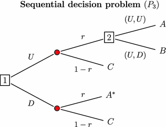
SDP
The other propositions’ proofs are available in the Appendix.
First order stochastic dominance (FOSD) is assumed in the whole proof.
Cooperation is represented by the fact the present self is dictating a change of preference to the future self by making an initial act of faith by choosing \(U\) instead of \(D\) at the initial node.
However, the tractability of GBI is not proven in this paper’s framework and such general frame could be useful in this purpose.
All three decision nodes tree (\(3\times 3\) trees) can be represented in this form when assuming RCL.
Without DC, an additional hypothesis could be done in order to prove the result: Consequential FOSD : \(\forall A, A^{*} \in \varDelta (X) A\) consequentially stochastically dominates \(A^{*}\), if and only if \(\forall r \in [0,1] (A, r; {\overline{0}}, {\overline{1-r}}) \succ A^{*}\).
Assuming consequential FOSD, \((A, r; {\overline{0}}, {\overline{1-r}}) \succ A^{*}\rightarrow c(A, r; {\overline{0}}, {\overline{1-r}}) > c(A^{*})\)
-
\(\rightarrow \) \((c(A, r; {\overline{0}}, {\overline{1-r}}),r;C,1-r ) \succ (c(A^{*}),r;C,1-r )\) by FOSD.
-
\(\rightarrow \) \((c(A, r; {\overline{0}}, {\overline{1-r}}),r;C,1-r ) \succ (A^{*},r; C,1-r)\) by RCL.
-

References
Allais, M. (1953). Le comportement de l homme rationnel devant le risqueâ: Critique des postulats et axiomes de l ecole amèricaine. Econometrica, 21, 503–546.
Bardsley, N., Cubitt, R., Loomes, G., Moffat, P., Starmer, C., & Sugden, R. (2010). Experimental economics: Rethinking the rules. Princeton: Princeton University Press.
Bradley, R. (2009). Becker’s thesis and three models of preference change. Politics, Philosophy & Economics, 8(2), 223–242.
Burks, A. W. (1977). Chance, cause, reason. Chicago: University of Chicago Press.
Cubitt, R. P., Starmer, C., & Sugden, R. (1998). Dynamic choice and the common ratio effect: An experimental investigation. The Economic Journal, 108(450), 1362–1380.
Gauthier, D. (1997). Resolute choice and rational deliberation: A critique and a defense. Noûs, 31(1), 1–25.
Hammond, P. J. (1988). Consequentialist foundations for expected utility. Theory and Decision, 25, 25–78.
Hammond, P. J. (1989). Consistent plans, consequentialism, and expected utility. Econometrica, 57(6), 1445–1449.
Hazen, G. B. (1987). Does rolling back decision trees really require the independence axiom? Management Science, 33(6), 807–809.
Hey, J., & Lotito, G. (2009). Naive, resolute or sophisticated? A study of dynamic decision making. Journal of Risk and Uncertainty, 38(1), 1–25.
Kahneman, D., & Tversky, A. (1979). Prospect theory: An analysis of decision under risk. Econometrica, 47, 263–291.
Karni, E., & Safra, Z. (1989). Dynamic consistency, revelations in auctions and the structure of preferences. The Review of Economic Studies, 56(3), 421–433.
Karni, E., & Schmeidler, D. (1991). Atemporal dynamic consistency and expected utility theory. Journal of Economic Theory, 54(2), 401–408.
Kreps, D. M., & Porteus, E. L. (1978). Temporal resolution of uncertainty and dynamic choice theory. Econometrica, 46(1), 185–200.
LaValle, I. H., & Wapman, K. R. (1986). Rolling back decision trees requires the independence axiom!. Management Science, 32(3), 382–385.
Machina, M. J. (1989). Dynamic consistency and non-expected utility models of choice under uncertainty. Journal of Economic Literature, 27(4), 1622–1668.
McClennen, E. F. (1990). Rationality and dynamic choice: Foundational explorations. Cambridge: Cambridge University Press.
Nebout, A., & Dubois, D. (2012). When allais meets ulysses: Dynamic consistency and the certainty effect. Working Papers 09-30, LAMETA, University of Montpellier.
Nebout, A., & Willinger, M. (2012). Categorizing behavioral strategies: an individualized experiment. Work in progress, LAMETA, University of Montpellier.
Nielsen, T. D., & Jaffray, J.-Y. (2006). Dynamic decision making without expected utility: An operational approach. European Journal of Operational Research, 169(1), 226–246.
O’Donoghue, T., & Rabin, M. (1999). Doing it now or later. The American Economic Review, 89(1), 103–124.
Rabinowicz, W. (1995). To have one’s cake and eat it, too: Sequential choice and expected-utility violations. Journal of Philosophy, 92(11), 586–620.
Raiffa, H. (1968). Decision analysis—Introductory lectures on choices under uncertainty. Reading, MA: Addison-Wesley.
Sarin, R., & Wakker, P. (1994). Folding back in decision tree analysis. Management Science, 40(5), 625–628.
Sarin, R., & Wakker, P. P. (1998). Dynamic choice and nonexpected utility. Journal of Risk and Uncertainty, 17(2), 87–119.
Seidenfeld, T. (1988). Decision theory without “independence” or without “ordering”. Economics and Philosophy, 4(2), 267–290.
Siniscalchi, M. (2011). Dynamic choice under ambiguity. Theoretical Economics, 6(3), 379–421.
Strotz, R. H. (1955). Myopia and inconsistency in dynamic utility maximization. The Review of Economic Studies, 23(3), 165–180.
Volij, O. (1994). Dynamic consistency, consequentialism and reduction of compound lotteries. Economics Letters, 46(2), 121–129.
von Neumann, J., & Morgenstern, O. (1947). Theory of games and economic behavior (2nd ed.). Princeton: Princeton University Press.
Wakker, P. (1999). Justifying Bayesianism by dynamic decision principles. Working paper, Medical Decision Making Unit, Leiden University Medical Center, The Netherlands.
Acknowledgments
I am deeply grateful to Jean-Yves Jaffray for his precious help, advises and support on this work. I am also grateful to Brian Hill, Chris Starmer, and Marc Willinger, to participants in conferences in Chicago, Paris and Bilbao and in seminars in University of Queensland and Aix-Marseille School of Economics for their helpful comments. I also thank an anonymous referee for his constructive comments and suggestions on earlier drafts of this paper.
Author information
Authors and Affiliations
Corresponding author
Appendix
Appendix
1.1 Conceptual summary
See Table 2.
1.2 Machina’s classification
Machina (1989) provides another extension of the static violation of the independence axiom by using the common consequence effect.
However he ends up with a categorization of individuals that is similar to ours:
-
\(\alpha \)-\(people\) who are EU maximizers and whose underlying preferences verify independence and therefore separate in all aspects.
-
\(\beta \)-\(people\) who are non-Eu maximizers and CON such individuals are non-DC.
-
\(\gamma \)-\(people\) who are non-Eu maximizers and non-CON such individuals are DC.
Another category of people studied by Machina is the dynamically consistent non-EU maximizers who use BI to determine their optimal strategy in a SDP. They are called \(\delta \)-\(people\) and Machina argues that that the use of this procedure is not normatively defendable in the case of non-EU maximizers.
Machina’s criticisms are legitimate. However, this paper investigates more deeply the \(\gamma \)-\(people\) and proposes a general kind of folding back procedure which could escape these normative criticisms and have a strong descriptive power.
1.3 Generalized backward induction (GBI)
If a CON-sophisticated agent is aware of the influence of forgone event on his preferences, he can take it into account when implementing the folding back procedure. More precisely, the folding back procedure is in general thought to apply at each decision node on elements of \(\varDelta (X)\), here a procedure is considered which applies at each decision node to elements of \({\overline{\varDelta }}(\varDelta (X))\).
An example of SDP is displayed in Fig. 5 Footnote 30 in order to describe how a CON-sophisticated agent applies GBI procedure to this problem:
-
First, the agent looks at decision node 3 where he has to choose between \(A\) and \(B\). He knows that his choice will be influenced by the resolution of the prior lottery, therefore to determine which prospect he will choose at node 3, he has to evaluate \((A,r_{2}; {\overline{C_{2}}},{\overline{1-r_{2}}})\) versus \((B,r_{2}; {\overline{C_{2}}},{\overline{1-r_{2}}}) \) rather that \(A\) versus \(B\). Let say he prefers \((A,r_{2}; {\overline{C_{2}}},{\overline{1-r_{2}}})\) and note \(EC_{2}\) the certainty equivalent of this prospect.
-
Then at decision node 2, the agent replaces (using folding back procedure) the upper branch by \(EC_{2}\) and therefore has (by the same reasoning than in decision node 3) to evaluate prospects \((EC_{2},r_{1}; {\overline{C_{1}}},{\overline{1-r_{1}}})\) versus \((D,r_{1}; {\overline{C_{1}}},{\overline{1-r_{1}}})\). Let say he prefers this last prospect and note \(EC_{1}\) its certainty equivalent.
-
Finally, the individual arrives at the actual decision (decision node 1) and have only to choose there between \(E\) and \(EC_{1}\).
Remark
It could be argued that this procedure does not take into account the possibility for the course in the decision tree to end up in \(C_{1}\) or \(C_{2}\). Actually it does as soon as the decision maker is dynamically consistent because in this case he does not make any difference for the uncertainty to be resolved prior or after his decision. (i.e. prospects \((A,r_{2}; {\overline{C_{2}}},{\overline{1-r_{2}}})\) and \((B,r_{2}; {\overline{C_{2}}},{\overline{1-r_{2}}})\) are ranked the same way than \((A,r_{2}; C_{2},1-r_{2})\) and \((B,r_{2}; C_{2},1-r_{2})\).

General sequential decision problem
1.4 Proof of the propositions
In the dynamic problems four different one stage lotteries have been used: \(A, A^{*}, B\) and \(C\). For \(X \in \varDelta (X), c(X) \in X\) denotes the certainty equivalent of lottery \( X\) which mean that \((c(X),1) \sim X\). For the sake of simplicity, the following convention is used \((c(X),1)=c(X)\in \varDelta (X)\) (therefore here \(c(B)=x_{2})\).
The choice patterns between \(P_{1}\) and \(P_{2}\) reveal the following functional orderings:
-
Choosing \(U_{1}\) in \(P_{1}\) means that \(U_{1}\succ D_{1}\) which reveals that: \(V(A, r; {\overline{C}}, {\overline{1-r}})>V(B, r; {\overline{C}}, {\overline{1-r}})\).
-
Choosing \(U_{2}\) in \(P_{2}\) means that \(U_{2}\succ D_{2}\) which reveals that: \(V(A^{*}, r; C, 1-r)>V(B, r; C, 1-r)\).
Proof of Proposition 1
The agent we are interested in this proposition is either EU or non-RCL, therefore he satisfies both CON and DC and use BI.
(i) Let me prove that if he chooses \([U_{1}/U_{2}]\) in \(P_{1}/P_{2}\), this agent has to choose \((U,U)\) in \(P_{3}\).
First choosing \(U_{1}\) in \(P_{1}\) reveals that \(V(A, r; {\overline{C}}, \overline{1-r})>V(B, r; {\overline{C}}, \overline{1-r})\).
Assuming CON it also reveals that \(V(A)>V(B)\) (i.e. \(A\succ B\)) and so that \(c(A)>c(B)\).
If he chooses \(U\) at the first decision node, the agent knows that he will end up choosing the strategy \((U,U)\) by CON and BI because \(V[(U,U)]=V(c(A),r;C,1-r)>V(c(B),r;C,1-r)=V(U-D)\).
To complete his reasoning, he compares strategy \((U,U)\) with strategy \(D\) given that:
-
\(V[(U,U)]= V(c(A),r;C,1-r )\).
-
\(V(D) = V(A^{*},r;C,1-r)\).
Assuming FOSD, \(A \succ A^{*} \rightarrow (c(A),1)=c(A)\sim A\succ A^{*}\)
-
\(\rightarrow (c(A),r; {\overline{C}}, {\overline{1-r}}) \succ (A^{*},r; {\overline{C}}, {\overline{1-r}})\) by CON.
-
\(\rightarrow \) \((c(A),r; C, 1-r) \succ (A^{*},r; C,1-r)\) by DC.
-
\(\rightarrow \) \(V[(U,U)]>V(D)\).
(ii) Let me prove that an agent who chooses \([D_{1}/D_{2}]\) in \(P_{1}/P_{2}\), chooses \((U,D)\) in \(P_{3}\).
First choosing \(D_{1}\) in \(P_{1}\) reveals that \(V(B, r; {\overline{C}}, {\overline{1-r}})>V(A, r; {\overline{C}}, {\overline{1-r}})\).
Assuming CON it also reveals that \(V(B)>V(A)\) (i.e. \(B\succ A\)) and \(c(B)>c(A)\).
If he chooses \(U\) at the first decision node, the agent knows that he will end up choosing the strategy \((U,D)\) by CON and BI because \(V[(U,D)]=V(c(B),r;C,1-r)>V(c(A),r;C,1-r)=V[(U,U)]\).
To finish his reasoning, he compares strategy \((U,D)\) with strategy \(D\) given that:
-
\(V[(U,D)] = V(c(B),r;C,1-r )= V(B,r;C,1-r \)) (\(B=c(B)\) here).
-
\(V(D) = V(A^{*},r;C,1-r)\).
The choice of \(D_{2}\) in \(P_{2}\) reveals that \(V(B, r; C, 1-r)>V(A^{*}, r; C, 1-r)\) therefore \(V[(U,D)]>V(D)\). \(\square \)
Proof of Proposition 2
The agent we are interested in this proposition is non-CON, therefore he satisfies both RCL and DC and uses GBI as he is sophisticated.
(i) Let me prove that an agent who chooses \([U_{1}/U_{2}]\) in \(P_{1}/P_{2}\), chooses \((U,U)\) in \(P_{3}\).
First choosing \(U_{1}\) in \(P_{1}\) reveals that \(V(A, r; {\overline{C}}, {\overline{1-r}})>V(B, r; {\overline{C}}, {\overline{1-r}}) \rightarrow \)
\(c(A, r; {\overline{C}}, {\overline{1-r}})>c(B, r; {\overline{C}}, {\overline{1-r}})\). If he chooses \(U\) at the first decision node, the agent knows that he will end up choosing the strategy \((U,U)\) by using GBI because \(V[(U,U)]=V(c(A, r; {\overline{C}}, {\overline{1-r}}),r;C,1-r)>V(c(B, r; {\overline{C}}, {\overline{1-r}}),r;C,1-r)=V[(U,D)]\).
To complete his reasoning, he compares strategy \((U,U)\) with strategy \(D\) given that:
-
\(V[(U,U)] = V(c(A, r; {\overline{C}}, {\overline{1-r}}),r;C,1-r )\).
-
\(V(D) = V(A^{*},r;C,1-r)\).
But \(V(c(A, r; {\overline{C}}, {\overline{1-r}}),r;C,1-r )=V([(A, r; {\overline{C}}, {\overline{1-r}}),r;C,1-r] )\) by RCL.
And \(V([(A, r; {\overline{C}}, {\overline{1-r}}),r;C,1-r] )=V((A,r; C, 1-r))\) by DC.Footnote 31
(ii) Let me prove that an agent who chooses \([D_{1}/D_{2}]\) in \(P_{1}/P_{2}\), chooses \((U,D)\) in \(P_{3}\).
First choosing \(D_{1}\) in \(P_{1}\) reveals that \(V(B, r; {\overline{C}}, \overline{1-r})>V(A, r; {\overline{C}}, \overline{1-r})\) \(\rightarrow \)
\(c(B, r; {\overline{C}}, {\overline{1-r}})>c(A, r; {\overline{C}}, {\overline{1-r}})\).
If he chooses \(U\) at the first decision node, the agent knows that he will end up choosing the strategy \((U,D)\) by using GBI because \(V[(U,D)]=V(c(B, r; {\overline{C}}, {\overline{1-r}}),r;C,1-r)>V(c(A, r; {\overline{C}}, {\overline{1-r}}),r;C,1-r)=V[(U,U)].\)
To complete his reasoning, he should now compare strategy \((U,D)\) with strategy \(D\) given that:
-
\(V[(U,D)] = V(c(B, r; {\overline{C}}, {\overline{1-r}}),r;C,1-r )\).
-
\(V(D) = V(A^{*},r;C,1-r)\).
But \(V(c(B, r; {\overline{C}}, {\overline{1-r}}),r;C,1-r )=V([(B, r; {\overline{C}}, {\overline{1-r}}),r;C,1-r] )\) by RCL.
And \(V([(B, r; {\overline{C}}, {\overline{1-r}}),r;C,1-r] )=V((B,r; C, 1-r))\) by DC.
The choice of \(D_{2}\) in \(P_{2}\) reveals that \(V(B, r; C, 1-r)>V(A^{*}, r; C, 1-r)\) therefore \(V[(U,D)]>V(D)\). \(\square \)
Proof of Proposition 3
The agent we are interested in this proposition is non-CON, therefore he satisfies both RCL and DC. However, he is naïve and therefore use BI as if he was EU.
(i) Let me prove that such an agent who chooses \([U_{1}/U_{2}]\) in \(P_{1}/P_{2}\), chooses \(D\) in \(P_{3}\).
First choosing \(U_{1}\) in \(P_{1}\) reveals that \(V(A, r; {\overline{C}}, {\overline{1-r}})>V(B, r; {\overline{C}}, {\overline{1-r}})\). However, because he is non-CON for these prospects he also prefers \(B\) to \(A\), so \(V(B)>V(A)\). If he chooses \(U\) at the first decision node, the agent knows that he will end up choosing the strategy \((U,U)\) by using BI, because \(V[(U,D)]=V(c(B))>V(c(A))=V[(U,U)]\).
To complete his reasoning, he compares strategy \((U,D)\) with strategy \(D\) given that:
-
\(V[(U,D)]= V(c(B),r;C,1-r )=V(B,r;C,1-r )\).
-
\(V(D) = V(A^{*},r;C,1-r)\).
The choice of \(U_{2}\) in \(P_{2}\) reveals that \(V(B, r; C, 1-r)<V(A^{*}, r; C, 1-r)\) therefore \(V[(U,D)]<V(D)\) from the point of view of decision node 1.
\(\rightarrow \) the CON-naïve agent ends up revealing behavioral strategy \(D\).
(ii) Let me prove that such an agent who chooses \([D_{1}/D_{2}]\) in \(P_{1}/P_{2}\), chooses \((U,D)\) in \(P_{3}\).
First choosing \(U_{1}\) in \(P_{1}\) reveals that \(V(B, r; {\overline{C}}, {\overline{1-r}})>V(A, r; {\overline{C}}, {\overline{1-r}})\). However, because he is non-CON for these prospects he also prefers \(A\) to \(B\), so \(V(A)>V(B)\). If he chooses \(U\) at the first decision node, the agent knows that he will end up choosing the strategy \((U,U)\) by using BI, because \(V[(U,U)]=V(c(A))>V(c(B))=V[(U,D)]\).
To complete his reasoning, he compares strategy \((U,U)\) with strategy \(D\) given that:
-
\(V[(U,U)] = V(c(A),r;C,1-r )=V(A,r;C,1-r )\).
-
\(V(D) = V(A^{*},r;C,1-r)\).
Using FOSD and RCL, \(V[(U,U)]>V(D)\). So the naïve agent will choose \(U\) at decision node 1 thinking he is implementing strategy \((U,U)\), but after the resolution of the prior risk, he will in fact choose \((U,D)\) at decision node 2 (as revealed by his choice of \(D_{1}\) in \(S_{1}\)).
\(\rightarrow \) the CON-naïve agent ends up revealing behavioral strategy \((U,D)\). \(\square \)
Proof of Proposition 5
(i) First, let me consider the case of naïve agent. He is non-DC (here he chooses the pattern \([D_{2}/U_{1}]\) in \(P_{1}/P_{2}\)) but he is not aware of this inconsistency when he deals with SDP by using BI reasoning.
Therefore, when evaluating the strategies \((U,U)\) and \((U,D)\) from the point of view of decision node 2 (i.e. prospects \((A, r; {\overline{C}}, {\overline{1-r}})\) vs \((B, r; {\overline{C}}, {\overline{1-r}})\)), he thinks he will end up choosing \(D\) because he is not aware of his inconsistency (the fact he chooses \(U_{1}\) in \(P_{1}\)).
To complete his reasoning, he should now compare strategy \((U,D)\) with strategy \(D\) given that:
-
\(V[(U,D)] = V(B,r;C,1-r )\).
-
\(V(D) = V(A^{*},r;C,1-r)\).
The choice of \(D_{2}\) in \(P_{2}\) reveals that \(V(B, r; C, 1-r)>V(A^{*}, r; C, 1-r)\) therefore \(V[(U,D)]>V(D)\) from the point of view of decision node 1.
So the naïve agent will choose \(U\) at decision node 1 thinking he is implementing strategy \((U,D)\), but after the resolution of the prior risk he has to choose at decision node 2, he will in fact choose \((U,U)_{}\) as revealed by his choice of \(U_{1}\) in \(S_{1}\).
\(\rightarrow \) the naïve agent ends up revealing behavioral strategy \((U,U)\).
(ii) Let me pursue with the case of the sophisticated agent. He is non-DC (he chooses the pattern \([D_{2}/U_{1}]\) in \(S_{1}/S_{2}\)) and he is aware of it. To resolve the SDP he uses BI reasoning taking into account the fact that his preferences are non-DC.
So, when looking at decision node 2, he is aware of the fact that he will choose \((U, U)\) given his dynamic preference (\(U_{1}\) in \(P_{1}\)). So he knows that the behavioral strategy he will implement if he chooses \(U\) at decision node 1 will be \((U,U)\).
To complete his reasoning, he should now compare strategy \((U,U)\) with strategy \(D\) given that:
-
\(V[(U,U)] = V(A,r;C,1-r )\).
-
\(V(D) = V(A^{*},r;C,1-r)\).
Using FOSD and RCL, it is clear that \(V[(U,U)]>V(D)\).
\(\rightarrow \) the sophisticated agent ends up revealing behavioral strategy \((U,U)\).
The last case is the one of the resolute agent. He is non-DC (he chooses the pattern \([U_{1}/D_{2}]\) in \(P_{1}/P_{2}\)) and he is aware of his inconsistency. However, he is able to force and binds himself to fight against this inconsistency. Using backward induction reasoning and taking into account his inconsistency he knows he will end up choosing the behavioral strategy of the sophisticated agent \((U,U)\).
Here, as there is no problem of domination of the behavioral strategy of the sophisticated agent, the resolute agent can choose between the two undominated strategies \((U,U)\) and \((U,D)\) whether it is the present self who has the negotiation power \((U,D)\) or the future self \((U,U)\). \(\square \)
1.5 CRE-oriented categorization

Experimental test of DC

Sequential decision problem (\(P_{3}\))
Rights and permissions
About this article
Cite this article
Nebout, A. Sequential decision making without independence: a new conceptual approach. Theory Decis 77, 85–110 (2014). https://doi.org/10.1007/s11238-013-9387-y
Published:
Issue Date:
DOI: https://doi.org/10.1007/s11238-013-9387-y