The non-ideal theory of the Aharonov–Bohm effect

Abstract

Elay Shech and John Earman have recently argued that the common topological interpretation of the Aharonov–Bohm (AB) effect is unsatisfactory because it fails to justify idealizations that it presupposes. In particular, they argue that an adequate account of the AB effect must address the role of boundary conditions in certain ideal cases of the effect. In this paper I defend the topological interpretation against their criticisms. I consider three types of idealization that might arise in treatments of the effect. First, Shech takes the AB effect to involve an idealization in the form of a singular limit, analogous to the thermodynamic limit in statistical mechanics. But, I argue, the AB effect itself features no singular limits, so it doesn’t involve idealizations in this sense. Second, I argue that Shech and Earman’s emphasis on the role of boundary conditions in the AB effect is misplaced. The idealizations that are useful in connecting the theoretical description of the AB effect to experiment do interact with facts about boundary conditions, but none of these idealizations are presupposed by the topological interpretation of the effect. Indeed, the boundary conditions for which Shech and demands justification are incompatible with some instances of the AB effect, so the topological interpretation ought not justify them. Finally, I address the role of the non-relativistic approximation usually presumed in discussions of the AB effect. This approximation is essential if—as the topological interpretation supposes—the AB effect constrains and justifies a relativistic theory of the electromagnetic interaction. In this case the ends justify the means. So the topological view presupposes no unjustified idealizations.

1 Introduction

In a number of recent papers, Elay Shech (2015, (2018a, (2018b, (2019) and John Earman (2019) have argued for a re-evaluation of the AB effect, a phenomenon in the quantum theory of electromagnetically charged particles. They argue that more careful consideration of the effect can teach us lessons about foundational issues in physics and about modelling and idealization in science more generally. On their view, important facts about functional analysis are too often “swept under the carpet as a ‘merely technical’ issue” (Shech 2018a, p. 4841); in particular, they claim, physicists and philosophers have not sufficiently attended to the domains of definition of relevant operators. These conclusions about foundations of physics lead to conclusions about modelling and idealization. In this paper I dispute their foundational points and argue that the topological interpretation of the AB effect does not involve unjustified or unusual idealizations.

Shech and Earman both level complaints against the “topological view” of the AB effect; this view is Shech’s explicit target, while Earman criticizes a general class of analyses to which the topological view belongs. The AB effect can be seen when operating a beam of electrons in the neighborhood of a magnet. Even if you perfectly shield the magnet—so that the electric and magnetic fields near the beam both vanish—the behavior of your electron beam will covary with the magnetic field inside the magnet. This is striking: facts inside the magnet seem to be making a difference to the electron beam at a distance, unmediated by the intervening magnetic field. Topological explanations of this effect appeal to the fact that the region outside the magnet has a “hole” in it where the magnet should be, and argue that in the presence of such a hole, the electric and magnetic fields to not capture all the electromagnetic facts.¹ Shech isn’t convinced. He argues that this picture of a “hole” in space is an idealization and that if we relax the idealization then the topological explanation no longer works. On Shech’s view, understanding the AB effect means attending to the details of this idealization—especially to the electron beam’s interaction with the magnet’s shielding. In this he agrees with Earman, who complains that the philosophical literature has neglected the role of unitarily inequivalent representations of the canonical commutation relations in modelling the idealized shielding.

I think a version of the topological view is correct and that Shech and Earman are barking up the wrong tree; details about the shielding belong under the proverbial rug. It’s true that no realistic shielding is perfect, and it’s true that a careful mathematical analysis of an electron’s interaction with an ideal shield means digging into delicacies of functional analysis. But neither of these things is relevant to modelling the AB effect on the topological view. Indeed, on the topological view the AB effect occurs whether or not there is any shielding. The perfect shield in the last paragraph was mostly for drama, much like the moon’s negligible atmosphere can be used for a striking demonstration of Galileo’s law of free fall. In Sect. 2 I argue that the topological view’s reference to a hole in space doesn’t involve any idealization—some things, like donuts, just have holes. To illustrate this, I describe the topological view in some detail, reconstructing Aharonov and Bohm’s (1959) original description of the effect as a proposal for a crucial experiment to resolve an ambiguity in the quantum theory of charged particles: are all of the electromagnetic facts captured by the electric and magnetic fields, or is there something more? More precisely: do two electromagnetic potentials represent the same physical state of affairs when they are gauge equivalent or when they have the same field strength? In this experimental context, topological features of the apparatus are essential for this “something more” to have an experimental signature, but these features aren’t idealizations.

Now we’ve read our Duhem, so we know that there are no crucial experiments; Aharonov and Bohm’s experiment relies on auxiliary assumptions, and alternative theories of the experiment are always logically possible. In Sect. 3 I consider whether the idealizations about the shielding that concern Shech and Earman can be found in these auxiliary assumptions or alternative theories. On one reading, Shech criticizes the topological view for failing to justify the assumption that imperfections in the magnet’s shielding will have a negligible effect. On this reading his comments are complementary to the topological view: the latter isn’t in the business of justifying this assumption about shielding, and the functional analysis facts he cites provide the topological view with a response to the skeptic who questions this assumption. On another reading, Shech may be proposing an alternative explanation of the behavior of charged particles near a magnet. This alternative explanation would be of the kind that Earman promotes—though, as Earman argues, justifying these assumptions about the shielding is only part of a complete explanation of the AB effect. On this reading we face a straightforward case of contrastive underdetermination. Idealizations arise on both readings, but they are the garden variety that arise whenever theory meets experiment.

In the final section I address the idealization of the electron as a non-relativistic particle. Earman complains that most discussions of the AB effect are set in “the bastardized theory in which a quantized electron is subjected an external classical electromagnetic field” (2019, p. 2013). He claims that this theory is inappropriate for foundational study twice over: the electromagnetic field is really quantum, and the electron is really an excitation in a field. From the point of view of quantum field theory these are idealizations, and discussions of the AB effect do make them. They are also essential for the AB effect to play the role the topological view grants it. As I argue in Sect. 4, the topological view conceives of the AB effect as a signpost on the way to a quantum theory of the electromagnetic field: in the non-relativistic and large-mass limit, any such theory must reproduce the AB effect. In this case idealization is essential to the project of constraining the low-energy limit of quantum field theory, but it is only an idealization from the point of view of the more fundamental theory.

2 Essential idealizations

Shech charges the topological view with baldfaced absurdity: on his reconstruction, the view says that a single spacetime region both has a hole and does not have a hole. As I argue in this section, this isn’t a plausible reconstruction of the topological view. In addition to its absurdity, Shech’s reconstruction neglects the aim of the view. The purpose of the AB effect is to inform us of the “Significance of electromagnetic potentials in the quantum theory”, as Aharonov and Bohm’s title says. They identify an ambiguity in the quantum theory of a charged particle and develop a crucial experiment to resolve the ambiguity. The topological view is meant to supply a theoretical context in which this experiment can be seen as crucial and a basis for justifying future developments of the quantum theory of the electromagnetic interaction. In this section I give a more detailed statement of the topological view to demonstrate that it involves no singular limits.

On Shech’s reconstruction, the topological view is committed to a set of inconsistent claims. The behavior of an electron beam in the vicinity of a magnet will depend on electromagnetic facts inside the magnet, even when the beam doesn’t intersect the magnet and the facts inside the magnet have a negligible effect on the electric and magnetic fields outside of it. In particular, differences inside the magnet will correspond to different interference patterns on a photographic plate exposed to the beam. In quantum mechanics, interference patterns are explained by relative phases between different parts of the wavefunction. The topological view links the phase in the AB effect to the fact that the region outside the magnet is topologically nontrivial: it has a “hole” where the magnet should be. Shech reconstructs this view as committed to four claims:

• 1. Real systems consist of a simply connected electron configuration space.

• 2. Real systems display the AB effect.

• 3. The AB effect occurs if and only if there is a non-trivial relative phase factor.

• 4. A non-trivial relative phase factor arises if and only if the electron configuration space is non-simply connected. (Shech 2018a, p. 4847)

He argues further that these claims are in tension: “[w]hile the first two propositions imply that real systems are simply connected and display the AB effect, the last three propositions convey that real systems are non-simply connected in virtue of displaying the AB effect” (Shech 2018a, pp. 4847–4848). If this is right, then the topological view is internally incoherent and should be rejected.

This reconstruction of the topological view is motivated in part by Shech’s desire to assimilate the AB effect to the philosophical literature on singular limits. The classic example of a singular limit occurs in discussions of how we are to give a statistical mechanical underpinning for phenomenological thermodynamics. In thermodynamics, a phase transition—such as ice melting or water boiling—is characterized by a discontinuous jump in quantities like entropy. According to the usual statistical-mechanical reduction recipe, the entropy is a derivative of the partition function, which is an function of the number of particles in the statistical-mechanical model of the system. A discontinuous jump in the entropy therefore leads to a singularity in the partition function. But it turns out that the partition function can only be singular when the number of particles is infinite. So we have the following set of inconsistent claims:

• 1. Real systems have finite[ly many particles]

• 2. Real systems display phase transitions

• 3. Phase transitions occur when the partition function has a singularity

• 4. Phase transitions are governed/described by classical or quantum statistical mechanics (Callender 2001, p. 549)

These claims are inconsistent, because the last three imply that real systems have infinitely many particles. You might respond to this inconsistency by rejecting the third claim: while it’s convenient to identify phase transitions with singularities in the partition function, it would be taking thermodynamics too seriously to insist that a system must exhibit a singularity to undergo a phase transition. Proponents of the third claim argue that the identification of phase transitions with singularities plays some essential role, often concluding that the fourth claim is false and thermodynamic behavior is emergent in a strong sense. On this essentialist view, an adequate statistical-mechanical model of phase transitions must involve an idealization in which the system has infinitely many particles.² Shech interprets the topological view as an essentialist view in this spirit.

Even if Shech’s dialectical motivations are taken into account, I do not recognize the topological view in his reconstruction. In particular, the topological view is not analogous to the view that the infinite-particle idealization is essential for an adequate treatment of phase transitions. For one thing, the topological view is not concerned with topological properties of a particle’s configuration space but with topological properties of spacetime regions.³ Of course, the possible configurations for a particle in some region are just the points of that region that the particle can occupy, so this is partially a verbal point. More substantively, Shech characterizes the topological view as involving an essential idealization because it treats the region outside the magnet as topologically nontrivial. It’s true that this topological nontriviality is essential to the topological view. But this isn’t an idealization, it’s just a fact. The region outside of a magnet encloses a hole occupied by the region containing the magnet, so it’s topologically nontrivial. To cast the topological view in an essentialist mold there would have to be some theory that modelled the region outside a magnet as topologically trivial, and there isn’t one. If the topological view involves an essential idealization, it’s not one that’s related to the topological facts.

Walking through the details of the topological view shows that it doesn’t involve essential idealizations anywhere else, either. To begin, recall Aharonov and Bohm’s motivation. They aim to answer a question in the theory of charged particulate matter: how should we model the electromagnetic field in this theory? If we work in coordinates the answer can be found in any textbook on electrodynamics, at least in the classical case. The action of a worldline x for a particle of mass m and charge q moving in an electromagnetic potential $A_{\mu }$ is

$$\begin{aligned} S_{A}(x) = \int d\tau \left( \frac{1}{2}m{\dot{x}}^{2} + q {\dot{x}}^{\mu } A_{\mu } \right) \end{aligned}$$

where the integral is taken over the interval parametrizing the worldline x and ${\dot{x}}^{\mu }$ is the worldline’s tangent vector. Interpreted as a coordinate expression, this integral has a sufficiently clear meaning for the prediction of the particle’s motion: the curve x is a map from some interval into spacetime that traces out the particle’s worldline, and the physically possible worldlines are the stationary points of the action $S_{A}$. To compute these stationary points it’s enough to know that m and q are real numbers and $A_{\mu }$ assigns a quadruple of real numbers to every point in spacetime. That is, it’s enough to know that four scalar fields can serve as coordinates for the space of electromagnetic fields. But any number of mathematical objects have such a coordinate expression, so this doesn’t tell us what we should take the electromagnetic field to be, mathematically speaking.

Computationally, a choice of mathematical model is a choice of which manipulations are permitted and which proscribed—in particular, it is a choice of legal substitutions. In our case there are three salient interpretations of the potential $A_{\mu }$, each having different substitution rules with respect to a choice of coordinates:⁴

• 1. The electromagnetic field is a covector field, and $A_{\mu }$ are the components of this covector field in a choice of coordinates. Two covector fields $A_{\mu }$ and $A'_{\mu }$ are inter-substitutable just in case $A_{\mu } = A'_{\mu }$ for all $\mu$.

• 2. The electromagnetic field is a principal U(1)-bundle equipped with a connection, and $A_{\mu }$ are the components of this connection in a choice of coordinates. Every U(1)-valued function g gives a substitution rule that replaces $A_{\mu }$ with . We say that two potentials $A_{\mu }$ and $A'_{\mu }$ are gauge equivalent if 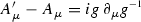for some U(1)-valued function g.⁵

• 3. The electromagnetic field is a field strength tensor $F_{\mu \nu }$, an antisymmetric (0, 2)-tensor, and the components of this tensor are a function of $A_{\mu }$:

  $$\begin{aligned} F_{\mu \nu } = \partial _{\mu }A_{\nu } - \partial _{\nu }A_{\mu } \end{aligned}$$

  Two sets of coordinates $A_{\mu }$ and $A'_{\mu }$ are inter-substitutable just in case they give rise to the same field strength tensor; in this case we’ll say that they’re equipotent.

These possibilities are ordered by the strictness of the corresponding substitution rule. The equivalence relation on the set of potentials generated by the first interpretation is just the identity relation, which is the finest equivalence relation. And the second interpretation generates a finer equivalence relation than the third, because gauge-equivalent potentials are always equipotent. So the ambiguity might make a practical difference by manifesting as an ambiguity about which substitutions are permissible.

Aharonov and Bohm register that in the classical case we can take the potential $A_{\mu }$ to represent the field strength tensor, as in the third interpretation. As they say, the potentials $A_{\mu }$ and $A'_{\mu }$ are interchangeable for all practical purposes if they generate the same field strength tensor $F_{\mu \nu }$. For consider the equations of motion induced by the action. A stationary worldline satisfies the Lorentz force law

$$\begin{aligned} q F_{\mu \nu } {\dot{x}}^{\nu } = m\ddot{x}_{\mu } \end{aligned}$$

and in the Newtonian framework this is everything: the free modelling parameter in this framework is the force appearing in Newton’s second law, and in this model it’s $qF_{\mu \nu }{\dot{x}}^{\nu }$. Since Newtonian forces suffice to model systems of this kind, we may suppose that the electromagnetic configuration is entirely captured by the field strength tensor $F_{\mu \nu }$. On this reading, two equipotent potentials represent the same configuration, much like the expressions 1/2 and 2/4 represent the same rational number.

The quantum-mechanical situation is different. The state of a quantum particle at time $t_{0}$ is given by a probability amplitude $\psi (t_{0}, x_{0})$, where the second coordinate ranges over all of space. The dynamics are given by an integral transform

$$\begin{aligned} \psi (t_{1}, x_{1}) = \int dx_{0} \int {\mathcal {D}}x\, e^{\frac{i}{\hbar }S(x)} \psi (t_{0}, x_{0}) \end{aligned}$$

integrating $\psi (t_{0}, x_{0})$ against a kernel defined by an integral over all paths x such that $x(t_{0}) = x_{0}$ and $x(t_{1}) = x_{1}$, weighted by a function of the classical action S and Planck’s constant $\hbar$. By contrast with classical matter, we have no reformulation of these dynamics purely in terms of forces. So in the quantum model of a charged particle we can’t demonstrate that the field strength tensor $F_{\mu \nu }$ tracks all the electromagnetic facts by moving to a framework where $F_{\mu \nu }$ is the only modelling parameter. This does not show that two equipotent potentials can give different dynamics, but it does prevent us from running an argument analogous to the argument we ran in the classical case.

All is not lost: in the quantum context we can still rule out the first interpretation of the potential—according to which it’s a covector field—because the dynamics, “as well as the physical quantities, are all gauge invariant” (Aharonov and Bohm 1959, p. 485). That is, for all practical purposes the physics is invariant under gauge equivalence, as in the interpretation of $A_{\mu }$ as a connection on a principal U(1)-bundle. If $A_{\mu }$ and $A'_{\mu }$ are gauge equivalent then the difference $S_{A'} - S_{A}$ in the actions they determine will be independent of the path. This means that the integral transforms they determine will differ by a constant phase, and because the probability amplitude is only defined up to a phase this means that $A_{\mu }$ and $A'_{\mu }$ determine the same quantum dynamics. So for all practical purposes, gauge-equivalent potentials are interchangeable.

To decide between the equivalence relations of the remaining two interpretations, we need a situation in which gauge-equivalent potentials are interchangeable but equipotent potentials are not. This is what Aharonov and Bohm provide. Such contexts necessarily involve a topologically nontrivial region—that is, a region that isn’t contractible. For if some region is contractible then the only principal U(1)-bundle over it is the trivial one, giving every principal U(1)-connection a global coordinate representation as a covector field $A_{\mu }$. And if $A_{\mu }$ and $A'_{\mu }$ are two equipotent potentials then the covector field $A'_{\mu } - A_{\mu }$ has vanishing field strength tensor, so by the Poincaré lemma there’s a U(1)-valued function g such that

which is to say that $A_{\mu }$ and $A'_{\mu }$ are gauge equivalent. Over a contractible region gauge equivalence coincides with equipotence, and there can be no experiments of the kind we seek.

Fig. 1

The double-slit experiment

A topologically nontrivial experiment is easy to find. Consider the paradigmatic double-slit experiment in Fig. 1. Electrons are emitted from a source, pass through two slits in a shield, and register on a detector screen. The kernel of the dynamics in this experimental setup can be separated into one integral over paths that pass through the slits and one over paths that intersect the shield:

$$\begin{aligned} \int \, {\mathcal {D}}x\, e^{\frac{i}{\hbar }S(x)} = \int _{\text {slits}} {\mathcal {D}}x\, e^{\frac{i}{\hbar }S(x)} + \int _{\text {shield}} {\mathcal {D}}x\, e^{\frac{i}{\hbar }S(x)} \end{aligned}$$

Treating the shield as an infinite potential barrier suppresses the second integral, so we can safely neglect it. Thus the dynamics are given by an integral over paths in the region outside the shield. This region is topologically nontrivial, because a loop around the bit of the shield between the slits can’t be contracted to a point while remaining in the exterior region.

To turn the double-slit experiment into our crucial experiment we only need to add an electromagnetic potential $A_{\mu }$ outside the shield. The kernel of the dynamics then becomes

$$\begin{aligned} \int _{\text {slits}}{\mathcal {D}}x\, e^{\frac{i}{\hbar }S_{A}(x)} \end{aligned}$$

This expression is gauge-invariant but can change if $A_{\mu }$ is replaced with an equipotent potential. For an illustration, consider the amplitude at time $t_{1}$ at the point $x_{1}$ on the screen collinear with the source and the point on the shield between the slits, and suppose that $A_{\mu }$ has vanishing field strength tensor. Then $S_{A}$ has the same stationary paths as the action of a free particle, since the classical equations of motion only involve the field strength tensor. If we suppose that the slits have vanishing width there are then two stationary paths, depicted in Fig. 1: a path $x_{\uparrow }$ that passes through the top slit and its reflection $x_{\downarrow }$ passing through the bottom slit. Treating the electron source as a point distribution means that the amplitude coincides with the kernel of the dynamics, and the stationary phase approximation tells us that in the small-$\hbar$ limit the amplitude is proportional to a sum over the stationary points of the action

$$\begin{aligned} \psi (t_{1}, x_{1}) \propto e^{\frac{i}{\hbar }S_{A}(x_{\uparrow })} + e^{\frac{i}{\hbar }S_{A}(x_{\downarrow })} \end{aligned}$$

The relative phase of these two terms is determined by

$$\begin{aligned} S_{A}(x_{\downarrow }) - S_{A}(x_{\uparrow }) = \int _{t_{0}}^{t_{1}} dt\, {\dot{x}}^{\mu }_{\downarrow }A_{\mu } - \int _{t_{0}}^{t_{1}} dt\, {\dot{x}}^{\mu }_{\uparrow }A_{\mu } \end{aligned}$$

since the paths have the same kinetic term. This is the integral of $A_{\mu }$ along the concatenation of and $x_{\downarrow }$, which encircles the portion of the shield between the slits. Since this loop isn’t contractible, this integral may not vanish. Indeed, it can be made to take any real value by an appropriate choice of a potential with vanishing field strength tensor.⁶ It follows that different electromagnetic potentials can lead to different amounts of interference between the two classical paths and thus different detection probability distributions over the screen, even when all of the potentials under consideration have the same field strength tensor.

Experiment can now decide between the principal connection and field strength tensor interpretation. Run a double-slit experiment in the presence of an electromagnetic field. If the potential is the coordinate expression of a principal connection then gauge-inequivalent but equipotent potentials will lead to different patterns on the detector screen; this is the AB effect. If there is no AB effect—that is, if equipotent fields always lead to the same wave pattern on the detector screen—then we can continue to use the coarser equivalence relation generated by the field strength tensor.⁷ Of course, as with any experiment there are implementation details. But insofar as we are concerned with the question of interpretation that Aharonov and Bohm set out to answer, these details are beside the point.

This positive characterization of the topological view in hand, return to Shech’s set of incompatible claims. The versions of these claims that the topological view actually endorses are something like the following.

• 1. There is a contractible spacetime region containing the AB apparatus.

• 2. The AB apparatus displays the AB effect.

• 3. The AB effect occurs if and only if there is a nontrivial phase factor.

• 4. A nontrivial phase factor arises only over a non-contractible region.

Only the fourth of these claims is distinctive of the topological view. Indeed, I take it that the fourth claim is constitutive of the topological view, alongside the theoretical context just reviewed in which the AB effect is a crucial experiment to license the “only”. The other three claims seem both true and uncontroversial. The laboratory room containing the AB apparatus is contractible. The second claim is empirical, and its truth settles Aharonov and Bohm’s motivating question. The quantum-mechanical explanation for the effect appeals to the phase between the paths through the top slit and those through the bottom one, as in every explanation of the wave patterns observed in a double-slit experiment, so the third claim is a commitment to modelling the particulate matter quantum-mechanically. These four claims are non-contradictory, and on the topological view they’re true. In particular, there is no contradiction between the fact that the inside of the room containing the AB apparatus is contractible while the region outside the shield isn’t; different regions can have different properties.

Shech’s general critique of the topological view fails, because the topological view is not committed to the inconsistent set of claims he attributes to it. He thinks that the view fails “to tell a story about why the idealized AB effect, conventionally defined so as to necessitate a [non-simply-connected] configuration space, has anything to do with the concrete AB effect as it is manifested in the laboratory” (2018a, p. 4845). But this is just the story on offer: the region of the laboratory outside the shield is topologically nontrivial. So on the topological view, the AB effect doesn’t involve any idealizations about spacetime regions, nor does my presentation appear to involve essential idealizations about anything else. But I glossed over the idealization that Shech and Earman are mainly concerned with when I said that we could neglect contributions from paths that intersect the shield. Unlike the topological features of the magnet’s exterior, this is an idealization, and for all I’ve said it’s the kind of infinite idealization that interests Shech. Now I’ll argue that it’s not.

3 Ancillary idealizations

In light of the last section, Shech’s complaint against the topological view seems to misfire. He finds the topological view inadequate because it fails to address details of the experimental implementation that Aharonov and Bohm propose—in particular, details about the shield. Earman, too, complains that the philosophical literature doesn’t “show much awareness of the subtleties required to implement the idealizations involved in the AB effect” (2019, p. 2017). But from the perspective of the topological view, it’s hard to see why these details are relevant. There are two possibilities. If the complaint is only that the topological view doesn’t address these details then so be it; Shech and Earman’s comments are friendly supplements to the view. But some of their remarks seem to be arguments against the interpretation of the AB effect mooted in Sect. 2. That is, they may instead be arguing that the field strength tensor does indeed capture all the electromagnetic facts.

The topological view envisions the AB effect as a crucial experiment. On a naive reading, this means that there are two possible contradictory outcomes, one of which is deductively entailed by the principal connection interpretation and the other by the field strength tensor interpretation. The outcome of the experiment confirms one interpretation and falsifies the other. There are therefore two kinds of objections to the topological view. A narrow objection might accept the topological view’s theoretical narrative but balk at its claims about the empirical facts. The topological view is silent on the battery of auxiliary assumptions required to actually test the AB effect, and you might worry that the AB effect has never in fact been realized in the laboratory. Such worries might concern the realization of the necessary electromagnetic fields, the magnitude of the effect, or similar. More broadly, you might reject the topological view’s framing entirely. That is, you might argue that the principal connection interpretation and the field strength tensor interpretation aren’t the only two options.

We can read Shech and Earman’s remarks with either the narrow or broad objections in mind. The heart of their complaint is that the topological view doesn’t specify enough features of the AB experiment. In particular, the topological view doesn’t reckon with an ambiguity that arises in the context of infinite potential barriers. As an illustration of this ambiguity, consider a quantum particle confined to the interval [0, 1] by an infinite potential at either end. According to the Hamiltonian quantization recipe, the configuration space for this particle is the Hilbert space $L^{2}[0, 1]$ of square-integrable functions on [0, 1] and its dynamics are of the form

$$\begin{aligned} \psi (t_{1}) = e^{-i(t_{1} - t_{0})H} \psi (t_{0}) \end{aligned}$$

with H a densely-defined self-adjoint operator. Furthermore, on its domain H takes the form of the classical Hamiltonian with the momentum replaced by an operator acting as $-i\hbar \nabla$; in our case this means

$$\begin{aligned} H = -\frac{\hbar ^{2}}{2m}\nabla ^{2} \end{aligned}$$

with m the particle’s mass. Since H is unbounded and self-adjoint its domain must be some strict subset of the Hilbert space, but the quantization recipe gives us no guidance as to what this domain should be. So the Hamiltonian quantization recipe leaves the dynamics undefined; it tells us only how H acts, not what operator it is, and so we cannot exponentiate it to give the dynamics.

This is a real ambiguity, because in general there will be more than one self-adjoint operator satisfying the Hamiltonian quantization recipe’s requirements (Reed and Simon 1975, X.1). The Hamiltonian in the previous paragraph is naturally associated with many dense domains. We might choose a relatively small domain like the set of smooth functions with compact support in (0, 1), giving an operator $H_{\infty }$. Or we might choose a relatively large domain like the set of continuously-differentiable functions $\psi$ such that $H\psi$ is square-integrable, giving an operator $H^{*}_{\infty }$. We might also consider domains consisting of smooth functions that satisfy some boundary conditions. For example, choosing the Dirichlet boundary condition $\psi (0) = \psi (1) = 0$ gives an operator $H_{D}$, and choosing the Neumann boundary condition $\psi '(0) = \psi '(1) = 0$ gives an operator $H_{N}$. Not every choice of domain gives a self-adjoint operator: for example, the adjoint of $H_{\infty }$ is the distinct operator $H^{*}_{\infty }$. But some domains do give self-adjoint operators, like $H_{D}$ and $H_{N}$. Indeed, there are infinitely many self-adjoint operators on $L^{2}[0, 1]$ that act as H on their domain, each giving rise to distinct dynamics.

The discussion of Sect. 2 made no reference to the Hamiltonian’s domain, so Shech and Earman are right that the topological view doesn’t address this ambiguity. But it’s not obvious that this ambiguity needs addressing. As I argue in Sect. 3.1, it would be inappropriate for the topological view to address the difference between the Hamiltonians $H_{D}$ and $H_{N}$ because this difference isn’t relevant to the status of the electromagnetic field. The choice between $H_{D}$ and $H_{N}$ concerns how to model shielded magnets in particular experimental setups. It’s therefore of a piece with questions about how to model the source and screen in the double-slit experiment, and none of these are the topological view’s responsibility. However, changing the theoretical framing of the experiment might change our demands on an account of the AB effect. In Sect. 3.2 I consider an alternative framing that Shech and Earman might have in mind, according to which the AB experiment is set up to investigate a remote counterfactual world. Set in this frame, Shech and Earman are proposing an alternative to the topological view, but it’s hard to see what the virtues of this alternative are. Characterizing the AB apparatus as a “fictional system” Earman (2019, p. 1992) and the effect as one that “cannot be manifested in the laboratory” Shech (2018a, p. 4840) reduces it to a curiosity disconnected from the rest of our theorizing about electromagnetism.

3.1 Auxiliary assumptions

Shech argues “that the topological approach does not offer a satisfying justification for choosing the standard Dirichlet boundary conditions that pick out a unique self-adjoint extension of the Hamiltonian operator representing actual systems in which the AB effect manifests” (2018a, p. 4840). To fill this gap, Shech calls on a result of de Oliveira and Pereira (2008). Earman agrees with Shech that this is a gap that needs filling, adding that “[p]art of the justification is supplied by a pretty mathematical result, but also needed is a fleshing out of the idealization with additional stories about how the fictional attributes are realized” (2019, p. 1994).

It’s true that the topological view doesn’t try to justify Dirichlet boundary conditions, but it’s not a problem. Just the opposite: I take it to be an adequacy condition on an account of the AB effect that it not justify these boundary conditions. Boundary conditions play no role in the AB effect as described in Sect. 2, so pronouncing on them would be overstepping the bounds of the account. As an illustration, the rest of this subsection surveys the constellation of approximations, idealizations, and auxiliary hypotheses that surround the AB effect on the topological view. You can find boundary conditions here if you look hard enough, but the connection to the AB effect is severely attenuated. So attenuated, in fact, that the AB effect has no necessary connection to any specific boundary conditions—in particular, it does not require Dirichlet boundary conditions. So it’s a good thing the topological view doesn’t imply them.

The discussion of Sect. 2 was qualitative, rather than quantitative, because the topological view is an interpretation of the AB experiment. Qualitative characterization is one of the aims of interpretation, for a number of reasons. Quantitative descriptions issue from qualitative ones but not vice versa, in general. Moreover, the more we bind the AB effect to particular contexts, the less useful it is. If we understand the AB effect as a crucial experiment as the topological view suggests then we have learned something general about the electromagnetic interaction; if we understand it as the behavior of electrons in a particular apparatus we have learned something specific about a peculiar experimental setup. Relatedly, a qualitative analysis affords a more robust network of connections between the AB effect and the laboratory. If the AB effect were confined to the schematic cartoon of Fig. 1 then we would have no experimental access to it: among other things, there are more than two dimensions, and sources, shields, and screens have three-dimensional extensions. A qualitative story about the effect gives us other setups in which the effect manifests along with quantitative measures of how well some particular laboratory setup instantiates the schematic double-slit experiment of Fig. 1.

Because the topological view gives a qualitative account of the AB effect, it affords us necessary flexibility in choosing which approximations and idealizations to impose. The discussion of Sect. 2 was heavily approximate and idealized so as to avoid any explicit computations, but for convincing experiments the approximations must be better and the idealizations weaker. For the approximations and idealizations of our toy double-slit experiment, this is straightforward. Standard perturbation theory gives us the kernel of the dynamics to arbitrary order in $\hbar$, taking us well beyond the stationary phase approximation. Depending on what idealizations we impose, we may even be able to give a non-perturbative expression for the dynamics. We can replace the point distribution model of the electron source with something more realistic that depends on the source’s features, making the convolution nontrivial. A more realistic model of the slits in the screen would give them finite width, giving more paths over which to integrate when computing the perturbative expansion of the dynamics. We can also drop the assumption that the field strength tensor vanishes; indeed, the system will be influenced by the Earth’s electromagnetic field, the electron’s emission and absorption of stray Z bosons, and the gravitational influence of Sagittarius $\hbox {A}^{*}$.

If boundary conditions are relevant to the AB effect, they must appear somewhere on the spectrum described in the previous paragraph. It would be comically inappropriate to include gravitational corrections in an account of the AB effect. For conceptual or pedagogical purposes the level of description in Sect. 2 is adequate. It even suffices for the laboratory, if we characterize the AB effect as covariation of the interference fringes with the electromagnetic potential that goes beyond their covariation with the field strength. Higher orders of the dynamics or contributions from the finite size of the source and shield slits won’t create or obscure the effect, and all we need for confirmation of the AB effect is to see whether the interference fringes appreciably change when the magnetic flux changes with everything else held effectively constant. The de-idealizations in the previous paragraph are relevant if—and to the extent that—we can use them to help pin down the meanings of “appreciably” and “effectively” in this criterion of confirmation and respond to skeptical analyses of particular experiments.⁸ More formally, they are useful for estimating the magnitude of the effect and systematic errors. The size of the slits matters because it controls the envelope of the diffraction pattern. We can’t observe the AB effect in a double-slit apparatus with very large slits, but this isn’t disconfirmation; it’s an inappropriately high standard for significant observable differences. The gravitational influence of celestial bodies doesn’t matter, and it’s so weak that an informal order-of-magnitude estimate makes this obvious; the environment of an AB apparatus is effectively constant no matter what some star is doing. If Shech and Earman are right that the topological view neglects important details about boundary conditions, then there must be some boundary effect that threatens to swamp the size of the AB effect or generate significant systematic error. To respond to this worry we can step through the most salient idealizations and check that they pose no significant problems.

The idealizations in the setup of the double-slit experiment are inessential, according to the topological view. First, shields found in the laboratory will obviously be imperfect, so the kernel of the total dynamics will not be given by an integral over paths confined to the exterior region. For the AB effect to decide our crucial question we need only find some equipotent potentials $A_{\mu }$ and $A'_{\mu }$ such that

$$\begin{aligned} \int _{\text {slits}}{\mathcal {D}}x\, e^{\frac{i}{\hbar }S_{A'}(x)} \not = \int _{\text {slits}}{\mathcal {D}}x\, e^{\frac{i}{\hbar }S_{A}(x)} \end{aligned}$$

for then $A_{\mu }$ and $A'_{\mu }$ won’t be interchangeable. If all the shielding is perfectly good then these will be the only terms of the dynamics. If the shield is imperfect then the interference observed in the lab will also have contributions from paths that penetrate the shield. The second standard idealization sets the double slit experiment in two dimensions rather than three. The dominant contributions to the dynamics will be the classical paths, which lie in the plane of the source and slits, so the two-dimensional approximation will generally be good. But contributions from the dimension perpendicular to the page can be incorporated in the usual way as necessary.

So much for the approximations and idealizations of Sect. 2. That section’s discussion was also silent on many details of experimental implementation. For example, it simply assumed the possibility of a shield that could effectively prevent transmission of an electron beam. This is the proper attitude; as just noted, the topological view makes no quantitative claims about the details of the shielding, it supposes only that the contributions from paths that intersect the shielding can be effectively distinguished from the contributions from the paths of interest. The topological view must be consistent with effective shields, of course. For instance, if the shielding is effectively perfect then it must be acceptable to assume that the electron’s amplitude effectively vanishes at the shield. But this is compatible with the topological view, since the amplitude at the shield is given entirely by paths that intersect the shield. A more detailed treatment of the shield must appeal to facts about the shield itself. This might be a basic analysis in terms of reflection and transmission coefficients or might be a more detailed analysis that accounts for the material composition of the shield and the backscatter profile of electrons off a crystal of this kind. Either way, none of these details fall within the topological view’s remit.

In fact, the standard double-slit experiment itself is inessential. Good thing, too: the electron’s short wavelength means the slits, their separation, and the interference fringes would be impractically small in any experiment possible in Aharonov and Bohm’s time (Marton et al. 1954, p. 1100). I introduced this experiment in Sect. 2 as an illustration of an experiment in which a topologically nontrivial region is salient, and I chose it because it’s a familiar and paradigmatic example. But at the time Aharonov and Bohm were writing, electron interferometry had only recently become practical with Möllenstedt and Düker’s (1956) development of the electron biprism. This is the interferometry method Chambers (1960) used in the first experimental incarnation of the effect. Later tests use a modified double-slit setup proposed as a “crucial experiment” by Kuper (1980). In each case the region exterior to the shield and electromagnetic source is still topologically nontrivial, raising the possibility of equipotent but gauge-inequivalent potentials, and the interference pattern observed on the screen will be invariant under gauge equivalence but not equipotence. So, again, these alternative setups will exhibit an experimental signature of the principal connection interpretation of the potential, if it’s correct.

The same remarks apply just as well to the detector screen. The account of Sect. 2 leads to a particular quantum amplitude for the points on the screen, but experimental access to this amplitude is mediated by a choice of apparatus. Traditionally this would be a photographic plate, and a completely detailed analysis would require a story about how the quantum amplitude is transduced to a pattern on this plate. This might involve an analysis of the interaction between the incident electron and the silver halide in the photographic plate, the subsequent emission of an electron from the silver halide and absorption by a nearby silver ion, the development and fixing of the image, and so forth. Modern electron microscopes amplify and transduce the electron signal to a digital image in any number of ways, each of which would require their own analysis. These details are necessary for connecting the quantum amplitude to observation, but they’re not part of the AB effect.

We can run these changes one more time on the remaining piece of the AB experiment, the electromagnetic potential. The earliest experiments generated the requisite electromagnetic potentials either with a permanently magnetized iron whisker or a small solenoid. The solenoid affords a particularly nice qualitative picture of how you might generate equipotent but gauge-inequivalent potentials, since it can be found in any introductory textbook and supports a number of tricks for avoiding explicit computation. Suppose that the plane of Fig. 1 is transverse to the midpoint of a long, thin solenoid embedded in the shield at the point between the slits. Recall that near the midpoint of a long solenoid the magnetic field is constant and parallel to the axis of symmetry within the solenoid and vanishes outside of it. It follows that the electric field vanishes everywhere, so that the field strength tensor vanishes outside the solenoid. But by Stokes’ theorem the integral determining the relative phase of the upper and lower paths must be the magnetic flux through the solenoid’s interior. Since this will be constant and nonzero the potential outside the solenoid will be constant and nonzero as well, making it equipotent with but gauge-inequivalent to the vanishing potential. Schematically this is an illuminating picture, but in practice it’s hard to fabricate and compute the systematic error for. The potential from a ferromagnetic filament—or, better, toroid—is better suited to this purpose, and appears in more experimental implementations of the AB effect.⁹ Like the shield and the screen, a careful analysis of the electromagnetic potential must be able to account for the details of the magnet’s composition and inhomogeneities in the generated potentials. Thankfully, these details are yet again of little relevance to the topological view, which simply requests gauge-inequivalent equipotent potentials obtained in any which way.

The noodling in the last six paragraphs is meant to show by example that these experimental details just aren’t relevant to the topological view. It just doesn’t matter how you generate the electromagnetic potentials, or how you detect the predicted phase shift, or how you perform electron interferometry. It matters that you do these things if you’d like to confirm the AB effect, but the topological view won’t tell you what choices to make; these are determined by practical matters. It’s surely not the case that the topological view must explain how photographic plates work, nor is it a view about electron biprisms or permalloy toroids.

But these are just the grounds of Shech and Earman’s criticism: the topological view doesn’t justify a particular model of a shielded solenoid, and they think this a shortcoming. In particular, the topological view doesn’t give us a reason to make the domain of the Hamiltonian the set of smooth functions with Dirichlet boundary conditions at the shield. This is no surprise, since the topological view doesn’t talk about boundary conditions or solenoids. Boundary conditions didn’t even arise in the preceding discussion of satellite issues of experimental implementation. We skirted close to the context of this complaint when discussing the schematic solenoid that might generate the needed electromagnetic potential, but at that point we’d already ranged far from the topological view’s domain. It would be a mark against the topological view if it made specific recommendations about how to model solenoids, since few experimental realizations of the AB effect involve solenoids at all.

In fact, if the topological view justified Dirichlet boundary conditions then it would not merely be overstepping its bounds, it would be flatly wrong. Not only do boundary conditions lie outside the topological view’s purview, the boundary conditions that Shech and Earman want justified aren’t necessary for modelling the AB effect in the presence of a solenoid. On the topological view, the AB effect requires only that

$$\begin{aligned} \int {\mathcal {D}}x\, e^{\frac{i}{\hbar }S_{A'}(x)} - \int {\mathcal {D}}x\, e^{\frac{i}{\hbar }S_{A}(x)} \not = \int _{\text {shield}}{\mathcal {D}}x\, e^{\frac{i}{\hbar }S_{A'}(x)} - \int _{\text {shield}}{\mathcal {D}}x\, e^{\frac{i}{\hbar }S_{A}(x)} \end{aligned}$$

Boundary conditions might make a difference to the terms on the right hand side, but these are details the topological view leaves aside: if an apparatus instantiates this inequality then it instantiates the AB effect, and if it doesn’t it doesn’t. We shouldn’t demand that the right hand side be worked out using Dirichlet boundary conditions, because infinitely many other boundary conditions will do the job just as well. We could use Neumann boundary conditions, as Earman (2019, p. 2006) notes, and even more options become available if we lift the assumption of perfect shielding. It would be a problem for the topological view if it justified Dirichlet boundary conditions over Neumann boundary conditions, because that would wrongly tie the AB effect to irrelevant features of particular treatments of particular experimental realizations of the effect.

The topological view ought not justify Dirichlet boundary conditions when modelling a solenoid. So I think Shech can’t be right when he says that

it is exactly this type of work... that offers both an explanation of the AB effect as it manifests in the physical world, and a justification for appealing to the type of idealizations that arise in such a context. (2018a, p. 4851)

Shech envisions this work as analogous to the work you have to do in the thermodynamic context to justifiably reject the claim that phase transitions are singularities in the partition function. But the topological view does not appeal to any singularities. If an explanation of the AB effect requires a close study of the boundary conditions for the electromagnetic source then it also requires a close study of the boundary conditions for the shield and screen. If we choose to model these as infinite potential barriers then—as with any infinite barriers—we will encounter issues about domains of our operators. If a justification of these domains requires a physical story that refers to the composition of the source then it also requires a physical story about the metal composing the shield and the emulsion of silver salts on the photographic plate. These demands are implausibly weighty. But if they really are requirements then the topological view just doesn’t aim to explain the AB effect or justify the idealizations used to model a particular instantiation of the AB experiment, at least not by itself. It aims only to contribute a model of the interaction between a charged particle and an electromagnetic potential. An explanation of the AB effect will then join the topological view with the materials science that explains the behavior of the shield and the photochemistry that explains the behavior of the screen and the classical electrodynamics that explains the behavior of the electromagnetic source. Boundary conditions might enter in this last explanation, or they might not. If they do then this explanation is complementary to the topological view, which is concerned with a wholly separate part of the AB experiment.

3.2 Alternative interpretations

My reading of Shech and Earman in Sect. 3.1 must be wrong, since they mean to offer a competitor to the topological view rather than a complement. If we adopt the topological view then they seem to be attending to details of experimental implementation unrelated to the topological view, but they do not see their arguments this way. So perhaps we should reject the topological view’s framing of the matter. We can read Shech and Earman as proposing an alternative explanation of the AB effect, undermining its status as a crucial experiment by increasing the number of salient alternatives. In particular, they point out that the topological view assumes a kind of locality which you might question. If we remove this assumption then the AB effect is no longer a crucial experiment, and we need a new framing. Earman offers a holistic one on which the AB effect is an epiphenomenon and Aharonov and Bohm’s question cannot arise for realistic systems.

Earman suggests that we take the AB effect to answer a remote counterfactual: how would an electron behave in the vicinity of a perfectly shielded, infinitely long solenoid (2019, pp. 1994–1995)? The counterfactual nature of this question is emphasized by both: Shech remarks that “the AB effect cannot be manifested in the laboratory” (2018a, fn. 1) and Earman that “the target system in the AB effect is a fictional system” (2019, p. 1993). For both, the AB effect is a prediction about what would be observed in a world that lacks the limitations of our world’s matter and engineering. This world is very different from ours, but we might expect our theory of charged quantum matter to pronounce on it anyway. For Shech and Earman, the AB effect is one such otherworldly pronouncement. While the motivation for this counterfactual question is unclear, this reading seems to be behind some of the reception of the early tests of the AB effect, as Earman (2019, §7) explains.

The topological view gives a straightforward answer Earman’s counterfactual question because the topological view assumes that electromagnetism is local. More precisely, the salient options on the topological view are all separable: the electromagnetic state of some region determines and supervenes on the states of its subregions.¹⁰ Any geometric object over some region restricts to a geometric object over each of that region’s subregions, and if two geometric objects differ then there is some point at which they differ. We can therefore sensibly attribute an electromagnetic state to any given region on any of the three interpretations that the topological view considers, and this state will be independent of the states of regions disjoint from our region of interest. For a local theory of this kind, counterfactuals about worlds with nontrivial topologies are little different from counterfactuals about regions of our world with nontrivial topologies. So the topological view’s treatment of Earman’s counterfactual is more or less the discussion in Sect. 2.

Non-local theories can also answer this question, but the connection between theory and experiment is more involved. Both Shech and Earman seem to adopt a kind of holism on which there is one spatial region, one electron configuration space, one electromagnetic configuration space, and one indecomposable relation between the electromagnetic field’s configuration space and the electron’s dynamics. For example, they both speak of “the” configuration space of the electron. And as a result of this holism, the features of the AB effect, “although compatible with [quantum mechanics], are never realized in the actual world” (Earman 2019, p. 1993). The AB effect concerns the relationship between configurations of the electromagnetic field and the dynamics of an electron moving in that field. In particular, it concerns this relationship in the region outside a magnet. But if we adopt the suggested holism we are allowed only one spatial region, one electron configuration space, and one Hamiltonian per experiment. In particular, and contra the topological view, an electron moving outside of a solenoid can never inform us about the AB effect: the electron’s wavefunction will extend into the solenoid and we will be forced to attend to the electromagnetic field at every point of space. Or, at least, no electron can inform us about the AB effect on its own.

On a holistic view like this, predictions about worlds featuring infinite potentials must be obtained by appeal to a somewhat informal principle of continuity. As an illustration, return to the particle in an infinite potential well. On the holistic view this model is experimentally inaccessible because we can only generate finite potential barriers. That is, we only have experimental access to particles whose configuration space is of the form $L^{2}({\mathbb {R}})$. However, we can experimentally probe the particle in a box by considering a sequence of Hamiltonians of the form

$$\begin{aligned} H_{V} = {\left\{ \begin{array}{ll} -\frac{\hbar ^{2}}{2m}\nabla ^{2} &{} 0 \le x \le 1 \\ -\frac{\hbar ^{2}}{2m}\nabla ^{2} + V &{} \text {otherwise} \end{array}\right. } \end{aligned}$$

where V is some positive constant. It happens that in this case we can ignore questions about $H_{V}$’s domain, because there is an essentially unique choice that makes it self-adjoint. For any V we can test the predictions of quantum mechanics; for example, when V is very large the lowest levels of the particle’s energy spectrum will be approximately

$$\begin{aligned} E_{n} \simeq \frac{\hbar ^{2}}{2m}n^{2}\pi ^{2} \end{aligned}$$

with $E_{n}$ the nth energy level. In the limit of large V this approximate equality becomes exact for all n and coincides with the spectrum of the operator $H_{D}$ on $L^{2}[0, 1]$. So, you might argue, the Hamiltonian for a particle confined by infinite potentials is $H_{D}$, and we can test this by investigating particles whose Hamiltonian is $H_{V}$ for increasingly large V.

Both Shech and Earman seem to have a picture like this in mind, though they diverge on the details. Shech argues that a story like this applies in the case of the AB effect as well. The specifics differ: we are interested in square-integrable functions on the exterior of the shield, rather than those on the interval [0, 1], and the relevant Hamiltonians are more complicated.¹¹ But as Shech explains, the general picture is the same: we consider a family of “more realistic” Hamiltonians on $L^{2}({\mathbb {R}}^{3})$ parametrized by the strength of the shielding and then argue that in the limit of infinitely strong shielding we recover the analogue of $H_{D}$ on the Hilbert space of wavefunctions supported outside the shielding (2018a, p. 4848). So, he concludes, the correct explanation and understanding of the AB effect appeals to the existence and uniqueness of the domains making $H_{V}$ self-adjoint over $L^{2}({\mathbb {R}}^{3})$ combined with the behavior of these operators in the limit of large V.

Earman’s conclusion is more skeptical than Shech’s. Though he signs on to the same general picture, Earman demands some further justification of the principle of continuity. The problem is that the Hamiltonians $H_{D}$ and $H_{N}$ corresponding to Dirichlet and Neumann boundary conditions are both physically possible, and they give different physical predictions. The choice between them in any particular context is an empirical matter. As a consequence, the choice of limiting sequence is also an empirical matter. The original counterfactual question has no determinate answer on Earman’s version of the holistic view, because it doesn’t specify which sequences of worlds or states of the world we are to consider, nor the similarity relation that determines which of various possibilities counts as the one approximated by our laboratory investigations. That said, he grants that

while the details of the answer to the what-would-happen question may depend on how the details of the what-if scenario are filled in, the existence of observable effects in the behavior of the electron reflecting the strength of the magnetic flux inside the solenoid do not so depend (2019, p. 2007).

This more conservative version of the holistic view can’t give a fully detailed answer to the counterfactual question on the table, because this question is ill-posed by its lights. But it does assert that there will be a nontrivial phase shift of some kind.

It’s hard to find common ground between the topological view and the holistic one. The two views give the same answer to Earman’s counterfactual, so cannot be distinguished on that basis. And appealing to other features of the views are likely to presuppose the framing of one or the other. Does one of these views give a better explanation of the AB effect, though the predictions are the same? Shech and Earman can’t give a good explanation (says the topological view), because they don’t mention the most important feature of the AB effect: the difference between equipotence and gauge equivalence. Moreover, their discussion is too narrow and too broad: it is silent on actual instances of the AB effect—in which no infinite barriers appear—and applies just as well to systems with no interesting electromagnetic features, like a particle confined to a box or an ordinary double-slit experiment. Contrariwise (Shech and Earman might say), the topological view can’t account for the AB effect because its neglect of boundary conditions “hides a seething complexity in the different ways the Hamiltonian operator can be made self-adjoint” (Earman 2019, p. 2001). And it’s the topological view that’s too broad and too narrow, because it thinks that the AB effect can be manifested in the laboratory and does not assimilate it to other systems with infinite barriers.

If we follow Earman in taking the AB effect to concern the behavior of an otherworldly electron then we lose common ground on which to evaluate the topological view and the holistic alternative. On this framing the AB effect involves an idealized infinite solenoid by stipulation, making it essential to the effect in some sense, but on this limited definition any view must count it essential. Part of the disagreement over whether there is an essential idealization therefore concerns what counts as the AB effect. The two views give the same predictions in uncontroversial cases of the AB effect, and the virtues of each view only appear in the light of cases that the other view doesn’t count as an instance of the AB effect at all. Barring any internal incoherence in one view or the other, any choice between the two will be entangled with the choice of target domain and more general principles like locality.¹² So this is a case of contrastive underdetermination. But it’s an odd one, for it concerns two ways of justifying the answer to a remote, unmotivated counterfactual question. And from a perspective this general it’s not obvious what could be gained by resolving the underdetermination. However, on the topological view the stakes are high: the AB effect is central to our justification for the standard quantum model of the electromagnetic interaction.

4 The non-relativistic idealization

The topological view involves no essential idealization in the sense that interests Shech, but there’s idealization to be found in “the bastardized theory in which a quantized electron is subjected an external classical electromagnetic field” (Earman 2019, p. 2013). This setup idealizes away relativistic effects and quantum features of the electromagnetic field. But the topological view doesn’t claim that the AB effect would disappear if we adopted a more fundamental description of the system. Indeed, this is the point of taking the AB effect to be a “crucial experiment” in spite of the fact that there are non-local alternative interpretations. This is a typical use of “crucial” experiments. The point is not that the principal connection interpretation has no competitors, but that we may take the principal connection interpretation to be established for the purposes of further theory development. In particular, we can assume the principal connection interpretation when arguing about quantum theories of the electromagnetic interaction. And this is what the standard model of this interaction, quantum electrodynamics (QED), does. Rejecting the topological view means giving up part of the justification for QED and for specific applications of it. Of course, if the topological view is wrong then this supposed justification is merely apparent. But an alternative interpretation of the AB effect isn’t a true competitor to the topological view unless it can also play a comparable role in our story about QED.

I have been attributing to the topological view the idea that the AB effect is a crucial experiment, but this idea is fraught. As Duhem (1906, VI.3) argued, crucial experiments in the strict sense are impossible in physics: hypotheses in physics can never be tested in isolation but only alongside a whole system of hypotheses. Subjecting Aharonov and Bohm’s prediction to an experimental test as in Sect. 3.1 requires a host of hypotheses about the shield, screen, and sources, and many of these hypotheses concern electromagnetic behavior, which is exactly what we aim to be testing. And the AB effect can’t be strictly deciding between two options, because there are more than two possibilities. Plausibly, the features of this case are generic. Experiments require apparatus with their own theories, and logically possible alternatives lurk around every corner. So the topological view can’t be saying that the AB effect is a crucial experiment in this sense.

But there’s a different sense of “crucial experiment” on which the topological view can claim that the AB effect is crucial. This sense is reflected in any number of examples; for instance, return to the double-slit experiment.

• 1. The paradigmatic status of this experiment begins with Young, who first described it as a demonstration of destructive interference of light in lectures given in 1802 and 1803. He thought these experiments “simple and... demonstrative” (1804, p. 1) evidence for the wave theory of light over the emission theory, and later commentators often refer to these experiments as crucial. For example, Arago found these experiments so compelling that his 1832 encomium of Young sought in part to explain why all were not instantly converted to the wave theory.¹³

• 2. In 1819 the French Academy awarded a prize on the topic of diffraction. At the time, Laplace’s emission theory of light was dominant in France and on the prize committee: the only non-Laplacian judges were Arago and Gay-Lussac, and the latter’s interests lay outside optics. Fresnel’s winning memoir was a wave-theoretic treatment, and one of the Laplacian judges noted a simple consequence of Fresnel’s theory: the appearance of a spot of light at the center of a circular object’s shadow. Folklore has it that, despite the heavy opposition to the wave theory, “French resistance collapsed suddenly and relatively completely” (Kuhn 1962, p. 155) when Arago exhibited this white spot experimentally, and the committee bestowed Fresnel the award.¹⁴

• 3. Duhem illustrates the impossibility of a crucial experiment with Foucault’s 1850 measurement of the relative speed of light in air and water. Arago explicitly proposed this measurement as a crucial experiment meant to subject the emission and wave theories to “decisive tests” that would “unequivocally” decide whether light was composed of particles or waves (1838, p. 954, my translation).

In none of these three cases did the putatively crucial experiment lead to mass conversion; the wave theory became dominant in the 1830s, twenty years after Young’s experiment and twenty before Foucault’s. Nor did it lead to local conversion. Fresnel’s prize committee mentions the bright spot only briefly, and the word “wave” does not occur in their report. If any of the Laplacians on the prize committee converted to the wave theory, it was not before the 1830s. Nor was this lack of conversion obviously irrational. Young’s experiments were variations on Grimaldi’s well-known diffraction experiments from 1665, and emission theorists had developed their own story about destructive interference before Young came onto the scene. Moreover, the emission theory claimed crucial experiments of its own, which Newton marshalled in favor of his emission theory, and Young had no response to these. So none of these were crucial experiments in the strict sense. Nevertheless, all three are indeed crucial experiments in a relevant sense, at least if we adopt the wave theory of light.

Calling some experiment “crucial” means giving it a special theoretical status. As Lakatos often put it, the term “crucial” is an honorific. An experiment is crucial if it forcefully exhibits some important theoretical principle. These will necessarily be theory-bound. When Whewell says that Young’s work “certainly ought to have convinced all scientific men of the truth of [the wave theory]” (1837, p. 406) we should disagree on a historical reading of the claim: the wave theory was severely underpowered before Fresnel gave it a mathematical underpinning, and the emission theory had plenty of other successes. But we can also read Whewell—and Arago, in his encomium of Young—as claiming that Young’s experiments isolate one of the fundamental principles of the wave theory, and this is true. If only Young’s contemporaries had access to Fresnel’s developed theory (the sentiment goes), they would have realized the superiority of the wave theory once they were given the key empirical input of destructive interference. And now that we have this empirical result, the opening move for any defender of the wave theory ought to be an appeal to one of the experiments above, even though none of them logically compel agreement with the wave theory. Moreover, this is compatible with a multiplicity of crucial experiments. Arago was right in 1838 to say that an experiment like Foucault’s would be crucial, even though he had pronounced Young’s experiment crucial six years earlier. Finally, like most honors, the title of “crucial experiment” is granted at least as much to increase the prestige of the granting institution as to reward the recipient. The wave theory is superior because it can cleanly account for the above experiments, and these experiments are important because they demonstrate important physical principles of the wave theory of light.

The AB effect is crucial on the topological view in much the same way that Young’s double-slit experiment is crucial on the wave theory of light. The central principle of the topological view is that the electromagnetic field is represented better by a principal connection than a field strength tensor at the classical level, and one difference between these representations is clearly evinced in the AB effect. A necessary condition for this difference to arise is that the region under consideration be topologically nontrivial, like the region outside a magnet. Experimental setups with imperfect shielding are still instances of the AB effect, because they exhibit the difference between the principal connection interpretation and the field strength interpretation. Later work by Wu and Yang (1975) was necessary to consolidate the topological interpretation of the AB effect and to draw further conclusions based on it, much like Fresnel’s work was needed for the wave theory of light. But in light of this work, the empirical input of the nontrivial phase in an AB experiment is the grounds on which the topological view advises adopting the principal connection interpretation.

If we adopt the topological view then we can appeal to the AB effect for justification elsewhere. For example, consider the problem of quantizing gauge theories like electromagnetism. In his attempts to quantize general relativity Feynman used the simpler case of gauge theories as a testing ground. In both cases Feynman found he needed the ad hoc introduction of an “artificial, dopey particle” (1963, p. 710) to obtain physically sensible answers when calculating one-loop contributions to the dynamics. Subsequent work by Faddeev and Popov (1967)—later refined by Becchi et al. (1976) and Tyutin (1975)—showed that Feynman’s computations could be extended to the general case if we demand that the quantization procedure treat gauge-equivalent configurations in the same way. The topological view offers a justification for this demand: we know already from the AB effect that gauge equivalence is the correct substitution relation for gauge potentials, so our quantization procedures should respect this.¹⁵

From this perspective, Earman’s complaints about the “bastardized” setting of the AB effect lose their sting. The AB effect concerns the behavior of an electron in an electromagnetic field, where the electron is modelled as a quantum particle and the electromagnetic field as a classical field. Earman remarks that this setting is “infelicitous”, and that a “more appropriate context would be relativistic quantum field theory” (2019, p. 2016). Presumably the thought is that the AB effect is an issue in the foundations of physics, and therefore we should set our discussion in our most fundamental description of the system at issue. But on the topological view, the AB effect is part of the justification for our more fundamental theory of the electromagnetic interaction, because it constrains the classical limit of theory. And even if we forget about justification, QED presupposes that the principal connection interpretation is right and the field strength tensor interpretation wrong. QED lacks the ambiguity that Aharonov and Bohm set out to resolve, so we can’t devise an experimental context in which the AB effect would be informative.

This conception of the AB effect as a crucial experiment also helps identify why the topological view and Shech and Earman so often talk past each other. On the topological view, the AB effect demonstrates the principle that equipotent but gauge-inequivalent potentials represent distinct states of the electromagnetic field. The only relevant features of such a demonstration are those required for gauge equivalence and equipotence to come apart—namely, topological non-triviality. Shech and Earman’s diagnoses of the topological view’s problems presume a kind of holism on which we can only speak of one spacetime region, while the topological view assumes that the relevant theories are separable. Talk of infinite potentials and boundary conditions focuses on precisely the inessential features of the effect. No matter what we say about self-adjoint implementations of the Hamiltonian, and even if we say nothing at all, we will still be able to justify the usual approach to QED by appeal to the principle established by the AB effect. In short, the topological view gives a context such that the AB effect can serve as a premise. Shech and Earman’s treatment makes the AB effect the answer to a question, instead. And it’s hard to see why it’s a question of any interest.

5 Conclusion

I have sought to defend the topological view of the AB effect against Shech and Earman’s criticisms and to argue that the AB effect doesn’t involve idealization in any particularly interesting way. It is not relevantly analogous to the debate over the thermodynamic limit in statistical mechanics, because it involves no limits. You might model some features of an AB experiment using infinite limits. For example, you might model the screen or the shielding of the electromagnetic source as an infinite barrier. But these aren’t part of the AB effect. This is clear from the fact that the exact same issues arise when modelling the screen in an ordinary double-slit experiment for an uncharged particle. Infinite barriers in quantum mechanics may involve interesting questions of idealization, but the AB effect doesn’t involve infinite barriers. If there’s any sense in which the AB effect involves an idealization, it’s an idealization at the framework level. If the AB effect is to do its job in guiding the construction of a quantum theory of the electromagnetic interaction then it must appear in a regime that’s well-modelled by a theory we understand, like non-relativistic quantum mechanics. If we adopt a more fundamental theory, like QED, then the semiclassical setting of the AB effect is an idealization of a kind. But if we adopt QED then we’ve answered the question to be posed of the AB effect.

References

Aharonov, Y., & Bohm, D. (1959). Significance of electromagnetic potentials in the quantum theory. Physical Review, 115(3), 485.
Arago, F. (1838). Sur un système d’expériences à l’aide duquel la théorie de l’émission et celle des ondes seront soumises à des épreuves décisives. Comptes rendus des séances de l’Académie des Sciences, 7, 954–965.
Arago, F. (1857). Biographies of Distinguished Scientific Men (W. H. Smyth, B. Powell, and R. Grant, Trans.). Longman, Brown, Green, Longmans, and Roberts, London.
Bangu, S. (2009). Understanding thermodynamic singularities: Phase transitions, data, and phenomena. Philosophy of Science, 76(4), 488–505.
Batterman, R. W. (2003). Falling cats, parallel parking, and polarized light. Studies in History and Philosophy of Modern Physics, 34(4), 527–557.
Batterman, R. W. (2005). Critical phenomena and breaking drops: Infinite idealizations in physics. Studies in History and Philosophy of Modern Physics, 36(2), 225–244.
Batterman, R. W. (2011). Emergence, singularities, and symmetry breaking. Foundations of Physics, 41(6), 1031–1050.
Becchi, C., Rouet, A., & Stora, R. (1976). Renormalization of Gauge theories. Annals of Physics, 98(2), 287–321.
Bertlmann, R. A. (1996). Anomalies in quantum field theory. Oxford: Clarendon Press.
Boersch, H., Hamisch, H., & Grohmann, K. (1962). Experimenteller Nachweis der Phasenverschiebung von Elektronenwellen durch das magnetische Vektorpotential. II. Zeitschrift für Physik, 169(2), 263–272.
Butterfield, J. (2011). Less is different: Emergence and reduction reconciled. Foundations of Physics, 41(6), 1065–1135.
Callender, C. (2001). Taking thermodynamics too seriously. Studies in History and Philosophy of Modern Physics, 32(4), 539–553.
Chambers, R. G. (1960). Shift of an electron interference pattern by enclosed magnetic flux. Physical Review Letters, 5(1), 3–5.
de Oliveira, C. R., & Pereira, M. (2008). Mathematical justification of the Aharonov–Bohm Hamiltonian. Journal of Statistical Physics, 133(6), 1175–1184.
Dougherty, J. (2017). Sameness and separability in Gauge theories. Philosophy of Science, 84(5), 1189–1201.
Duhem, P. (1906). La Théorie Physique, Son Objet et Sa Structure. Paris: Chevalier & Riviére.
Earman, J. (2019). The role of idealizations in the Aharonov–Bohm effect. Synthese, 196(5), 1991–2019.
Faddeev, L. D., & Popov, V. N. (1967). Feynman diagrams for the Yang–Mills field. Physics Letters B, 25, 29–30.
Feynman, R. P. (1963). Quantum theory of gravitation. Acta Physica Polonica, 24, 697–722.
Fowler, H. A., Marton, L., Simpson, J. A., & Suddeth, J. A. (1961). Electron interferometer studies of iron whiskers. Journal of Applied Physics, 32(6), 1153–1155.
Healey, R. (2007). Gauging what’s real. Oxford: Oxford University Press.
Kuhn, T. S. (1962). The structure of scientific revolutions. Chicago: Chicago University Press.
Kuper, C. (1980). Electromagnetic potentials in quantum mechanics: A proposed test of the Aharonov-Bohm effect. Physics Letters A, 79(5–6), 413–416.
Lyre, H. (2004). Holism and structuralism in U(1) gauge theory. Studies in History and Philosophy of Modern Physics, 35(4), 643–670.
Marton, L., Simpson, J. A., & Suddeth, J. (1954). An electron interferometer. Review of Scientific Instruments, 25(11), 1099–1104.
Menon, T., & Callender, C. (2013). Turn and face the strange... ch-ch-changes: Philosophical questions raised by phase transitions. In R. Batterman (Ed.), The Oxford handbook of philosophy of physics (pp. 189–223). Oxford: Oxford University Press.
Möllenstedt, G., & Bayh, W. (1962). Kontinuierliche Phasenschiebung von Elektronenwellen im kraftfeldfreien Raum durch das magnetische Vektorpotential eines Solenoids. Physikalische Blätter, 18(7), 299–305.
Möllenstedt, G., & Düker, H. (1956). Beobachtungen und Messungen an Biprisma-Interferenzen mit Elektronenwellen. Zeitschrift für Physik, 145(3), 377–397.
Morrison, M. (2012). Emergent physics and micro-ontology. Philosophy of Science, 79(1), 141–166.
Myrvold, W. C. (2011). Nonseparability, classical, and quantum. The British Journal for the Philosophy of Science, 62(2), 417–432.
Nounou, A. M. (2003). A fourth way to the Aharonov–Bohm effect. In K. Brading & E. Castellani (Eds.), Symmetries in Physics: Philosophical Reflections (pp. 174–199). Cambridge: Cambridge University Press.
Palacios, P. (2018). Had we but world enough, and time... but we don’t!: Justifying the thermodynamic and infinite-time limits in statistical mechanics. Foundations of Physics, 48(5), 526–541.
Reed, M., & Simon, B. (1975). Methods of modern mathematical physics (Vol. II). Cambridge: Academic Press.
Shech, E. (2015). Two approaches to fractional statistics in the quantum Hall effect: Idealizations and the curious case of the Anyon. Foundations of Physics, 45(9), 1063–1100.
Shech, E. (2018a). Idealizations, essential self-adjointness, and minimal model explanation in the Aharonov–Bohm effect. Synthese, 195(11), 4839–4863.
Shech, E. (2018b). Infinite idealizations in physics. Philosophy Compass, 13(9), e12514.
Shech, E. (2019). Infinitesimal idealization, easy road nominalism, and fractional quantum statistics. Synthese, 196(5), 1963–1990.
Tonomura, A. (2010). The AB effect and its expanding applications. Journal of Physics A: Mathematical and Theoretical, 43(35), 354021.
Tonomura, A., Matsuda, T., Suzuki, R., Fukuhara, A., Osakabe, N., Umezaki, H., et al. (1982). Observation of Aharonov–Bohm effect by electron holography. Physical Review Letters, 48, 1443–1446.
Tonomura, A., Matsuda, T., Endo, J., Arii, T., & Mihama, K. (1986). Holographic interference electron microscopy for determining specimen magnetic structure and thickness distribution. Physical Review B, 34, 3397–3402.
Tyutin, I. V. (1975). Gauge invariance in field theory and statistical physics in operator formalism. Moscow: Lebedev Physics Institute.
Whewell, W. (1837). History of the inductive sciences (Vol. II). London: J. W. Parker.
Worrall, J. (1976). Thomas Young and the ‘refutation’ of Newtonian optics: A case-study in the interaction of philosophy of science and history of science. In C. Howson (Ed.), Method and appraisal in the physical sciences (pp. 107–179). Cambridge: Cambridge University Press.
Worrall, J. (1989). Fresnel, Poisson, and the white spot: The role of successful predictions in the acceptance of scientific theories. In D. Gooding, T. Pinch, & S. Schaffer (Eds.), The uses of experiment (pp. 135–157). Cambridge: Cambridge University Press.
Wu, T. T., & Yang, C. N. (1975). Concept of nonintegrable phase factors and global formulation of gauge fields. Physical Review D, 12, 3845–3857.
Young, T. (1804). Experiments and calculations relative to physical optics. Philosophical Transactions of the Royal Society of London, 94, 1–16.
Funding
Open Access funding enabled and organized by Projekt DEAL.
Author information
Authors and Affiliations
Corresponding author
Additional information
Publisher's Note
Springer Nature remains neutral with regard to jurisdictional claims in published maps and institutional affiliations.
Rights and permissions
Open Access This article is licensed under a Creative Commons Attribution 4.0 International License, which permits use, sharing, adaptation, distribution and reproduction in any medium or format, as long as you give appropriate credit to the original author(s) and the source, provide a link to the Creative Commons licence, and indicate if changes were made. The images or other third party material in this article are included in the article’s Creative Commons licence, unless indicated otherwise in a credit line to the material. If material is not included in the article’s Creative Commons licence and your intended use is not permitted by statutory regulation or exceeds the permitted use, you will need to obtain permission directly from the copyright holder. To view a copy of this licence, visit http://creativecommons.org/licenses/by/4.0/.
About this article
Cite this article
Dougherty, J. The non-ideal theory of the Aharonov–Bohm effect. Synthese 198, 12195–12221 (2021). https://doi.org/10.1007/s11229-020-02859-x
Received:
Accepted:
Published:
Issue Date:
DOI: https://doi.org/10.1007/s11229-020-02859-x