Evaluating Uncertainties in Coronal Electron Temperature and Radial Speed Measurements Using a Simulation of the Bastille Day Eruption

Abstract

Obtaining reliable measurements of plasma parameters in the Sun’s corona remains an important challenge for solar physics. We previously presented a method for producing maps of electron temperature and speed of the solar corona using K-corona brightness measurements made through four color filters in visible light, which were tested for their accuracies using models of a structured, yet steady corona. In this article we test the same technique using a coronal model of the Bastille Day (14 July 2000) coronal mass ejection, which also contains quiet areas and streamers. We use the coronal electron density, temperature, and flow speed contained in the model to determine two K-coronal brightness ratios at (410.3, 390.0 nm) and (423.3, 398.7 nm) along more than 4000 lines of sight. Now assuming that for real observations, the only information we have for each line of sight are these two K-coronal brightness ratios, we use a spherically symmetric model of the corona that contains no structures to interpret these two ratios for electron temperature and speed. We then compare the interpreted (or measured) values for each line of sight with the true values from the model at the plane of the sky for that same line of sight to determine the magnitude of the errors. We show that the measured values closely match the true values in quiet areas. However, in locations of coronal structures, the measured values are predictably underestimated or overestimated compared to the true values, but can nevertheless be used to determine the positions of the structures with respect to the plane of the sky, in front or behind. Based on our results, we propose that future white-light coronagraphs be equipped to image the corona using four color filters in order to routinely create coronal maps of electron density, temperature, and flow speed.

Appendices

Appendix A: Sources of Coronal Brightness

In Figure 10 we show two fundamental unavoidable sources of coronal brightness: the F- and K-coronal brightness, and their magnitudes, which extend from $1~\mbox{R}_{\odot }$ to $15~\mbox{R}_{\odot}$ from the Sun center. The polarized K-coronal models in Figure 10 were generated using Equation 1 in Reginald and Davila (2000) for electron temperature and speed of 1 MK and $0~\mbox{km}\,\mbox{s}^{-1}$, respectively, and two different electron density models by Baumbach (1937) and Leblanc, Dulk, and Bougeret (1998). The unpolarized and polarized F-coronal brightness are attributed to diffraction and reflection of photospheric light off coronal dust, respectively, and are from Koutchmy (1985). Here, it is evident that the F-coronal brightness begins to become partially polarized starting around $5~\mbox{R}_{\odot }$ from the Sun center. The unpolarized F-coronal brightness can be easily isolated by using linear polarizers or a polarization camera, as introduced in Reginald et al. (2017). However, separating the polarized F-coronal brightness from the polarized K-coronal brightness would be more challenging. In addition, this effort would be further compounded because we do not know the relative orientations of the polarized F and K components starting around $5~\mbox{R}_{\odot }$ to each other and may need modeling to separate the two. In any case, the polarized and unpolarized F-coronal brightness would both contribute toward the overall statistical noise in the measurements. The K-coronal brightness based on electron density as described in Leblanc, Dulk, and Bougeret (1998), generated using Equation 1 in Reginald and Davila (2000), crosses the F-coronal brightness around $2~\mbox{R}_{\odot }$, as commonly reported in the literature (see Figure 1 in Reginald et al., 2017).

Figure 10

F- and K-coronal brightness as a function of coronal height. The polarized K-coronal brightness plots were generated using the K-coronal model Equation 1 in Reginald and Davila (2000) for an electron temperature of 1 MK and an electron flow speed of $0~\mbox{km}\,\mbox{s}^{-1}$, respectively, and the two different electron density models by Baumbach (1937) and Leblanc, Dulk, and Bougeret (1998). The unpolarized and polarized F-coronal brightness is attributed to diffraction and reflection of photospheric light off coronal dust, respectively, and is from Koutchmy (1985).

In addition to the above sources of coronal brightness, experimenters have to contend with numerous other sources of brightness and instrumental limitations in their quest to measure the polarized K-coronal brightness. The prominent sources are listed below:

• i) Sky brightness: the sky brightness would be a factor depending on the location of the coronagraph, whether is operated within or outside the Earth’s atmosphere.

• ii) Diffraction: this is the amount of Sun light that comes around the occulter and contaminates the coronal brightness. It depends on the design of the coronagraph.

• iii) Vignetting: the amount of coronal light that is blocked by the occulter. Unfortunately, this is worst at the low coronal height of the image plane and again depends on the design of the coronagraph.

• iv) Internal scattering: all light entering the coronagraph is susceptible to scattering by the instrumental optics, and its magnitude is dependent on the transmission and reflection properties of the optical components.

• v) Dark current: this is an artificial brightness introduced by digital cameras and is a property of the charge-coupled device (CCD) used in the experiment.

These sources of brightness together with K and F will contribute toward reaching the full-well depth of the pixels in the CCD and will determine the duration of the exposure time. Collectively, the total signal measured by each pixel will contribute toward the total statistical noise in the measured K that will be used to measure the electron density, temperature, and speed.

Appendix B: Temperature-Dependent Temperature-Sensitive Brightness Ratio (T-TSBR)

The reason for the change in the temperature-sensitive filter ratio from (385.0, 410.0 nm) to (390.0, 410.3 nm) (see Section 4) is as follows:

• i) Modeled T-TSBRs based on the brightness ratio (410.0, 385.0 nm) for model solar wind speeds ranging from 0 to $1000~\mbox{km}\,\mbox{s}^{-1}$, as shown in Figure 11, were used to interpret the synthetic ISCORE experiment conducted on CORHEL-MAS data that contained only quiet regions and streamers (see Reginald et al., 2014). It is evident from Figure 11 that these modeled T-TSBRs match almost perfectly.

  Figure 11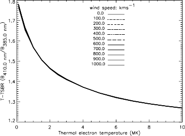

  

  Modeled T-TSBRs based on the brightness ratio 410.0 nm/385.0 nm for model solar wind speeds ranging from 0 to $1000~\mbox{km}\,\mbox{s}^{-1}$ in intervals of $100~\mbox{km}\,\mbox{s}^{-1}$. This model was used as modeled T-TSBR in Reginald et al. (2014) for a temperature interpretation of measured TSBR. Here, the line traces for the different line textures shown in the legend cannot be discerned, which proves that this brightness ratio is speed independent from 0 to $1000~\mbox{km}\,\mbox{s}^{-1}$. These models were generated using Equation 1 in Reginald and Davila (2000).

• ii) However, in the analysis presented in this article, the simulation data contain a powerful CME, which required extending the modeled T-TSBRs to wind speeds of up to $3000~\mbox{km}\,\mbox{s}^{-1}$. Figure 12, which is an extension of Figure 11 incorporating the extended T-TSBRs, shows that the modeled T-TSBRs start to deviate from the main curve for wind speeds above $1000~\mbox{km}\,\mbox{s}^{-1}$ in certain segments of the temperature range. Obviously, this deviation causes multiple temperatures to be attributed to certain temperature-sensitive intensity ratios.

  Figure 12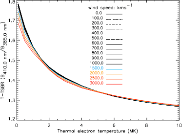

  

  Modeled T-TSBRs based on the brightness ratio 410.0 nm/385.0 nm for solar wind speeds from 0 to $3000~\mbox{km}\,\mbox{s}^{-1}$ in intervals of $100~\mbox{km}\,\mbox{s}^{-1}$ for the range $(0\,\mbox{--}\,1000)~\mbox{km}\,\mbox{s}^{-1}$ and $500~\mbox{km}\,\mbox{s}^{-1}$ for the range $(1000\,\mbox{--}\,3000)~\mbox{km}\,\mbox{s}^{-1}$. Here, Figure 11 is repeated with four more brightness ratios pertaining to speeds 1500, 2000, 2500, and $3000~\mbox{km}\,\mbox{s}^{-1}$, which are shown in color and are clearly seen to be speed dependent. These models were generated using Equation 1 in Reginald and Davila (2000).

• iii) The deviations shown in Figure 12 required searching for other possible brightness ratios that would produce a closely matching modeled T-TSBRs for solar wind speeds from 0 to $3000~\mbox{km}\,\mbox{s}^{-1}$. We found that the brightness ratio of 410.3 nm and 390.0 nm produced the best results, as shown in Figure 13, although small deviations remain (cf. Figure 13). In this article, the average of the modeled T-TSBRs shown in Figure 13 was used to interpret the brightness ratio between 410.3 nm and 390.0 nm for electron temperature (see Figure 5).

  Figure 13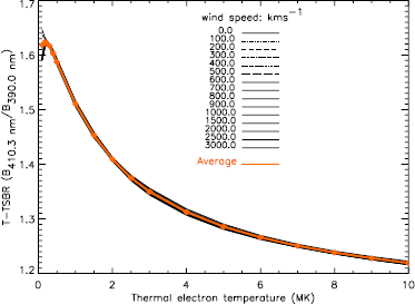

  

  Modeled T-TSBRs based on the brightness ratio 410.3 nm/390.0 nm for solar wind speeds from 0 to $3000~\mbox{km}\,\mbox{s}^{-1}$ in intervals of $100~\mbox{km}\,\mbox{s}^{-1}$ for the range $(0\,\mbox{--}\,1000)~\mbox{km}\,\mbox{s}^{-1}$ and $500~\mbox{km}\,\mbox{s}^{-1}$ for the range $(1000\,\mbox{--}\,3000)~\mbox{km}\,\mbox{s}^{-1}$. The average of the modeled T-TSBRs is used in Figure 5. Here, with the brightness ratio calculation based on two different wavelengths from Figures 11 and 12 gives a better convergence toward a speed-independent plot for speeds ranging from $(0\,\mbox{--}\,3000)~\mbox{km}\,\mbox{s}^{-1}$, and in this article, the curve passing through the average at each temperature position was used for temperature interpretation. These models were generated using Equation 1 in Reginald and Davila (2000).

Appendix C: Filter Selection

Identifying the central wavelengths of the filters and their shapes is very important for the success of the ratio technique described in this article. The two most important filter selection criteria are first, to obtain the steepest gradient in Figure 5 in the region of anticipated temperature measurement in order to minimize the error in temperature interpreted due to statistical noise in the measured TSBR, and second, to minimize the sensitivity of Figure 5 to speed in the region of anticipated speed measurements, in order to avoid non-singular values. Here, through an example, we explain how the above criteria are applied to select the optimum filters:

• i) First, we select filter profiles for two filters centered in the vicinity of the anti-nodes in Figures 2, 4, and 5 in Reginald et al. (2009). In this example, as shown in Figure 14, we select the two filters to be initially centered at 385.0 nm and 410.0 nm with bandwidths of 5.0 nm and 100% transmission.

  Figure 14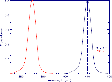

  

  Shapes of the temperature-sensitive filter profiles temporarily centered at 385.0 nm and 410.0 nm with FWHM of 5.0 nm.

• ii) Now, we need to identify the expected temperature and flow speed ranges we expect to measure in the coronal plasma. In this example, we expect to measure temperatures and flow speeds between (0.1 MK and 5.0 MK) and ($0.0~\mbox{km}\,\mbox{s}^{-1}$ and $500.0~\mbox{km}\,\mbox{s}^{-1}$), respectively. Here, the task is to find the most suitable central wavelengths of the two filters that would give the maximum spread in modeled T-TSBR along the $y$-axis in the selected temperature range that is also insensitive to speed in the selected speed range, as shown in Figure 5.

• iii) Then, we calculate the modeled T-TSBRs using model KCBSs generated for temperatures (0.1 and 5.0 MK) and speeds (0.0 and $500.0~\mbox{km}\,\mbox{s}^{-1}$) by sliding the shorter wavelength filter from 385.0 nm to 395.0 nm and the longer wavelength filter from 405.0 nm to 415.0 nm in intervals of 0.1 nm. The measured differences in T-TSBR for the two temperatures at the two speeds 0.0 and $500.0~\mbox{km}\,\mbox{s}^{-1}$ are shown in Figures 15 and 16, respectively. Here, the maximum differences are around positions C (385.5, 405.5 nm) and D (385.5, 414.0 nm) followed by A (393.0, 405.5 nm) and B (393.0, 414.0 nm). However, C and D are located at the blue end of the visible-light spectrum, and based on experience, this requires specialized coating on optics to minimize absorption and possibly a back-thinned CCD to improve the quantum efficiency. Then the next best regions are around A and B. The purpose of this step is to identify the regions with optimum differences in T-TSBR for the two extreme ends of the temperature range anticipated in the measurements.

  Figure 15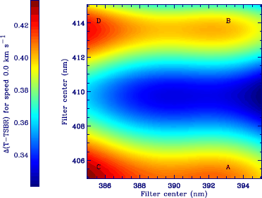

  

  Measured difference in T-TSBR between models with temperatures 0.1 MK and 5.0 MK with speed $0.0~\mbox{km}\,\mbox{s}^{-1}$.

  Figure 16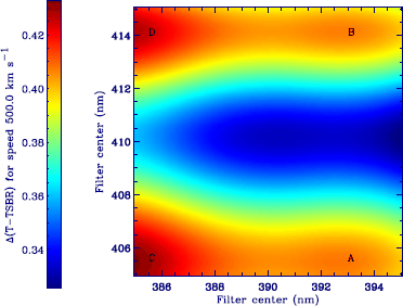

  

  Measured difference in T-TSBR between models with temperatures 0.1 MK and 5.0 MK with speed $500.0~\mbox{km}\,\mbox{s}^{-1}$.

• iv) Finally, we measure the difference between Figures 15 and 16 as shown in Figure 17. Here, we search for the regions where the differences are zero, indicating an independence of the modeled T-TSBRs to speed. Here, we see that region A (orange) is closer to zero than region B (green).

  Figure 17

  

  Difference between Figures 15 and 16.

• v) Based on these steps, we would select two filters centered at 405.5 nm and 393.0 nm to measure TSBR in the coronal plasma. The results of the modeled T-TSBR for temperatures between 0.1 MK and 5.0 MK and speeds between $0.0~\mbox{km}\,\mbox{s}^{-1}$ and $500.0~\mbox{km}\,\mbox{s}^{-1}$ are shown in Figure 18 and are clearly insensitive to speed in the desired range. These models were created for a coronal height of $3~\mbox{R}_{\odot }$. In Figure 18 the difference in T-TSBR in the $y$-axis is 0.41 ($1.57-1.16$), which is the value represented by A and B in Figures 15 and 16. However, from Figure 17 selecting B would have shown less independence from speed, and when used to interpret a measured TSBR for temperature, would have yielded multiple temperatures. In this exercise we therefore select A. This process can be reiterated for different shapes of the filter profiles while taking into account that a narrower filter will increase the integration time, and vice versa for a wider filter.

  Figure 18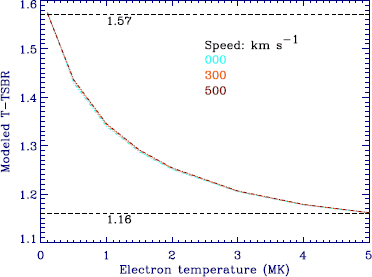

  

  Modeled T-TSBR as function of temperature between 0.1 MK and 5.0 MK and speeds between $0.0~\mbox{km}\,\mbox{s}^{-1}$ and $500.0~\mbox{km}\,\mbox{s}^{-1}$ using two filters centered at 393.0 nm and 405.5 nm.

References

Baumbach, S.: 1937, Astron. Nachr.263, 121. DOI .
Davila, J.M., Rabin, D.M., Reginald, N.L., Gong, Q., Shah, N., Chamberlin, P.C.: 2018, Spherical Occulter Coronagraph Cubesat. US Patent 9,921,099 B1, 20, 2018.
Fisher, R.R., Lee, R.H., MacQueen, R.M., Poland, A.I.: 1981, Appl. Opt.20, 1094. ADS . DOI .
Ichimoto, K., Kumagai, K., Sano, I., Kobiki, T., Sakurai, T., Munoz, A.: 1996, Publ. Astron. Soc. Japan48, 545. DOI .
Irada, I.S., Nasanova, L.P., Lisin, D.V., Popov, V.V., Krusanova, N.L.: 2017, J. Geophys. Res.122(1), 78. ADS . DOI .
Koutchmy, S.: 1985, G. Nikolsky memorial lecture. In: Properties and Interactions of Interplanetary Dust, 63. ADS .
Kurucz, R.L., Furenlid, I., Brault, J., Testerman, L.: 1984, Solar Flux Atlas from 296 nm to 1300 nm, National Solar Observatory, Arizona. ADS .
Leblanc, Y., Dulk, G.A., Bougeret, J.: 1998, Solar Phys.183, 165. ADS . DOI .
Linker, J., Török, T., Downs, C., Lionello, R., Titov, V., Caplan, R.M., Mikić, Z., Riley, P.: 2016, AIP Conf. Proc.1720, 020002. DOI .
Lionello, R., Linker, J.A., Mikić, Z.: 2009, Astrophys. J.690, 90. ADS . DOI .
Lionello, R., Mikić, Z., Linker, J.A.: 1999, J. Comput. Phys.152, 346. ADS . DOI .
Mann, I.: 1992, Astron. Astrophys.261, 329. ADS .
Manoharan, P.K., Tokumaru, M., Pick, M., Subramanian, P., Ipavich, F.M., Schenk, K., Kaiser, M.L., Lepping, R.P., Vourlidas, A.: 2001, Astrophys. J.559, 1180. ADS . DOI .
Mikić, Z., Linker, J.A.: 1994, Astrophys. J.430, 898. ADS . DOI .
Mikić, Z., Linker, J.A., Schnack, D.D., Lionello, R., Tarditi, A.: 1999, Phys. Plasmas6, 2217. ADS . DOI .
November, L.J., Koutchmy, S.: 1996, Astrophys. J.446, 512. ADS . DOI .
Reginald, N.L.: 2001, Ph.D. thesis. University of Delaware, Newark, USA, Publication Number: 9998766. ADS .
Reginald, N.L., Davila, J.M.: 2000, Solar Phys.195, 111. ADS . DOI .
Reginald, N.L., Davila, J.M., St. Cyr, O.C.: 2004, Solar Phys.225, 249. ADS . DOI .
Reginald, N.L., St. Cyr, O.C., Davila, J.M., Brosius, J.W.: 2003, Astrophys. J.599, 596. ADS . DOI .
Reginald, N.L., St. Cyr, O.C., Davila, J.M., Rabin, D.M., Guhathakurta, M., Hassler, D.M.: 2009, Solar Phys.260, 347. ADS . DOI .
Reginald, N.L., Davila, J.M., St. Cyr, O.C., Rabin, D.M., Guhathakurta, M., Hassler, D.M., Gashut, H.: 2011, Solar Phys.270, 235. ADS . DOI .
Reginald, N.L., Davila, J.M., St. Cyr, O.C., Rastatter, L.: 2014, Solar Phys.289, 2021. ADS . DOI .
Reginald, N.L., Davila, J.M., St. Cyr, O.C., Rabin, D.M.: 2017, J. Geophys. Res.122, 5856. DOI .
Reginald, N.L., Gopalswamy, N., Yashiro, S., Gong, Q., Guhathakurta, M.: 2017, J. Astron. Telesc. Instrum. Syst.3(1), 014001. ADS . DOI .
Riley, P., Lionello, R.: 2011, Solar Phys.270, 575. ADS . DOI .
Riley, P., Linker, J.A., Lionello, R., Mikić, Z.: 2012, J. Atmos. Solar-Terr. Phys.83, 1. ADS . DOI .
Saito, K., Makita, M., Nishi, K., Hata, S.: 1970, Ann. Tokyo Astron. Obs., Second Ser.12, 53. ADS .
Takahashi, N., Yoneshima, W., Hiei, E., Ichimoto, K.: 2000, The Last Total Solar Eclipse of the Millennium in Turkey, ASP Conf. Series205. ADS .
Thompson, W.T., Davila, J.M., Fisher, R.R., Orwig, L.E., Mentzell, J.E., Hetherington, S.E., Derro, R.J., Federline, R.E., Clark, D.C., Chen, P.T.C., Tveekrem, J.L., Martino, A.J., Novello, J., Wesenberg, R.P., St. Cyr, O.C., Reginald, N.L., Howard, R.A., Mehalick, K.I., Hersh, M.J., Newman, M.D., Thomas, D.L., Card, G.L., Elmore, D.F.: 2003, Proc. SPIE4853, 1. ADS . DOI .
Titov, V.S., Török, T., Mikić, Z., Linker, J.A.: 2014, Astrophys. J. arXiv . ADS . DOI .
Török, T., Downs, C., Linker, J.A., Lionello, R., Titov, V.S., Mikić, Z., Riley, P., Caplan, R.M., Wijaya, J.: 2018, Astrophys. J.856, 75. ADS . DOI .
Wang, T., Davila, J.M.: 2014, Solar Phys.289, 3723. ADS . DOI .
Acknowledgements
N.L.R. was supported by NASA grant PL10A-125. T.T. was supported by NSF’s FESD (Sun-2-Ice) and NASA’s LWS programs. Computational resources for the MHD simulation used in this article were provided by the NSF-supported Texas Advanced Computing Center (TACC) in Austin and the NASA Advanced Supercomputing Division (NAS) at Ames Research Center.
Author information
Authors and Affiliations
Corresponding author
Ethics declarations
Disclosure of Potential Conflicts of Interest
The authors declare that they have no conflicts of interest. Two of the authors, JD and NR, co-inventors of the US Patent cited in this article, declare that they have no conflicts of interest.