
Abstract
We consider the recent, very exceptional, 11-year cycle (2003 – 2009) of solar activity and confirm that the relative amplitude in rigidity spectrum, δD(R)/D(R), which can be approximated by a power law in rigidity R, of the first three harmonics of the 27-day variation of the galactic cosmic ray (GCR) intensity is hard in the maximum and soft in the minimum epochs of solar activity, as was found by neutron monitor data for the period of 1965 – 2002. This property is seen not only in separate minimum and maximum epochs but in individual intervals of a solar Carrington rotation as well: There exist many individual intervals of solar rotation when the expected rigidity spectrum of the 27-day variation of the GCR intensity indeed is hard in the maximum epoch of solar activity and is soft in the minimum epoch. We then construct a three-dimensional model of the 27-day variation of the GCR intensity based on Parker’s transport equation, by implementing in situ measurements of the changes in heliographic longitude of the solar wind velocity and interplanetary magnetic field for different epochs of solar activity.
1 Introduction
In previous papers (Gil and Alania, 2010, 2011) we have shown that the relative amplitude in rigidity spectrum, δD(R)/D(R), of the first, second, and third harmonics of the 27-day variation of the galactic cosmic ray (GCR) intensity (R is rigidity and δD(R)/D(R)∝R −γ) is hard in the maximum epochs and soft in the minimum epochs of solar activity (SA) for 1965 – 2002. It is of interest to study whether a similar behavior of the relative amplitude in the rigidity spectrum of the 27-day variation of the GCR intensity takes place in the period of 2003 – 2009, which includes the recent, very extraordinary minimum epoch of SA (e.g. Smith 2011; Leske et al. 2011; Gil, Modzelewska, and Alania 2012).
Our purpose in this paper is twofold.
-
i)
We wish to study changes of the exponent γ of the power-law of the rigidity spectrum, δD(R)/D(R), of the first three harmonics of the 27-day variation of the GCR intensity in the period of the recent outstanding 11-year cycle of SA (2003 – 2009), and some individual intervals of a Carrington rotation during maximum, intermediate, and minimum epochs of SA.
-
ii)
We want to construct a three-dimensional (3-D) theoretical model of the 27-day variation of the GCR intensity by implementing in situ measurements of the (heliographic) longitudinal changes of the solar wind velocity and interplanetary magnetic field (IMF) for maximum, intermediate, and minimum epochs of SA.
2 Experimental Data
We will study a long time series of daily data (1965 – 2009) from neutron monitors. An analysis of the long-period changes of the relative amplitude in rigidity spectrum of the first, second, and third harmonics of the 27-day variation of the GCR intensity needs data from neutron monitors with a track record of long term steadiness. Regrettably, merely few neutron monitors suit this condition. To use the data from two neutron monitors for the estimation of the reasonable rigidity spectrum exponent γ, there must be sufficient difference between the cut-off magnetic rigidity (R m). This requirement is acceptably satisfied by Kiel and Rome neutron monitors which we use in our analysis; for Kiel neutron monitor R m=2.29 GV and for Rome neutron monitor R m=6.32 GV. Ahluwalia and Fikani (2007) demonstrated that the median rigidity of the response of a detector can be used as an alternative to the cut-off rigidity. The median rigidity for the Kiel neutron monitor is 17 GV and for Rome it is 23 GV.
Calculations of the rigidity spectrum of the 27-day variation of the GCR intensity harmonics are based on the method presented in e.g. Dorman (1974) and Yasue et al. (1982),
where R max is the upper-limit rigidity beyond which the 27-day variation of the galactic cosmic ray intensity vanishes, and A is the amplitude of the 27-day variation of the GCR intensity for R=10 GV. After Wawrzynczak and Alania (2008, 2010) we take R max=100 GV, and then estimate the exponent γ.
The amplitudes of the first, second, and third harmonics of the 27-day variation of the GCR intensity in 1965 – 2009 are presented in Figures 1a, 2a, and 3a, respectively. Likewise, the calculated exponent γ in the relative rigidity spectrum of the first, second, and third harmonics of the 27-day variation of the GCR intensity in 1965 – 2009 are presented in Figures 1b, 2b, and 3b, respectively. In Table 1 are presented the values of the average exponents γ for all three harmonics of the 27-day variation of the GCR intensity for the minimum and maximum epochs of SA.

(a) Temporal changes of the amplitudes of the first harmonic of the 27-day variation of the GCR intensity by Kiel neutron monitor (NM). (b) The exponent γ of the rigidity spectrum of the first harmonic of the 27-day variation of the GCR intensity calculated using Kiel and Rome NMs in 1965 – 2009. The curves are smoothed over 39 Carrington rotations, with maximum epochs of solar activity (SA) marked with gray rectangles. At two maximum and minimum points the error bars are marked in orange.

(a) Temporal changes of the amplitudes of the second harmonic of the 27-day variation of the GCR intensity by Kiel NM. (b) The exponent γ of the rigidity spectrum of the second harmonic of the 27-day variation of the GCR intensity calculated using Kiel and Rome NMs in 1965 – 2009. The curves are smoothed over 39 Carrington rotations, with maximum epochs of SA marked with gray rectangles. At two maximum and minimum points the error bars are marked in orange.

(a) Temporal changes of the amplitudes of the third harmonic of the 27-day variation of the GCR intensity by Kiel NM. (b) The exponent γ of the rigidity spectrum of the third harmonic of the 27-day variation of the GCR intensity calculated using Kiel and Rome NMs in 1965 – 2009. The curves are smoothed over 39 Carrington rotations, with maximum epochs of SA marked with gray rectangles. At two maximum and minimum points the error bars are marked in orange.
Figures 1b –3b and Table 1 show that the relative amplitude in the rigidity spectrum of the harmonics of the 27-day variation of the GCR intensity is soft in the minimum epochs and hard in the maximum epochs of SA. Moreover, Figures 1 – 3 show a good anti-correlation between the amplitudes and the exponents γ for all the three harmonics of the 27-day variation of the GCR: The correlation coefficients are r=−0.702±0.021,−0.670±0.022, and −0.696±0.021 for the first, second, and third harmonics, respectively.
In order to construct a consistent model, an implementation of in situ measurements of solar wind parameters is required. Therefore, we consider some individual intervals of solar rotation in different epochs of SA. We analyze here the following 27-day intervals in the maximum, intermediate, and minimum epochs of SA: 23 October – 18 November 1991 (Figure 4), 10 July – 5 August 1994 (Figure 5), and 11 July – 6 August 1997 (Figure 6). The correlation coefficients between the changes of the GCR intensity I (measured by the Kiel neutron monitor) and the solar wind velocity, and between I and IMF strength B for each considered 27-day interval are presented in Table 2. The values of the exponent γ of the rigidity spectrum of the first harmonic of the 27-day variation of the GCR intensity for those particular intervals of the solar rotation are γ=0.56±0.19 in 1991, γ=1.06±0.17 in 1994, and γ=1.48±0.13 in 1997.

Daily changes of (a) the interplanetary magnetic field (IMF) strength B (green) and (b) the solar wind velocity (orange) in comparison with the GCR intensity (blue). The data are from the Kiel NM during one solar rotation in the maximum epoch of SA (23 October – 18 November 1991), and are smoothed over 3 days.

Daily changes of (a) the IMF strength B (green) and (b) the solar wind velocity (orange) in comparison with the GCR intensity (blue). The data are from the Kiel NM during one solar rotation in the moderate part of SA (10 July – 5 August 1994).

Daily changes of (a) the IMF strength B (green) and (b) the solar wind velocity (orange) in comparison with the GCR intensity (blue). The data are from the Kiel NM during one solar rotation in the minimum epoch of SA (11 July – 6 August 1997).
Table 2 shows that both the (heliographic) longitudinal changes of the solar wind velocity and the IMF strength should be the sources of the 27-day variation of the GCR intensity, with different contributions depending on the SA levels. It should be stressed that the 27-day variation of the GCR intensity in the minimum epochs is preferentially related to the solar wind velocity, while in the maximum epochs it is more related to the IMF strength. In a moderate level of SA both longitudinal changes of the solar wind velocity and the IMF strength simultaneously contribute to it. However, taking into account the complexity of the physical conditions in individual intervals of a solar rotation, there could be observed many cases which do not merely follow the above-mentioned characteristics.
3 Model of the 27-Day Variation of the GCR Intensity; Results and Discussion
We propose a model of the 27-day variation of the GCR intensity based on Parker’s (1965) transport equation:
where κ ij is the anisotropic diffusion tensor for 3-D magnetic field (Alania, 1978, 2002; Alania and Dzhapiashvili 1979), f is the omnidirectional distribution function in the interplanetary space, R is the rigidity of the GCR particles, U i =(U r ,0,0) is the solar wind velocity, and t is time. The symmetric part of the tensor κ ij describes diffusion in 3-D space, while the anti-symmetric part describes drift effects.
The general character of diffusion and drift of GCR is defined by the location and configuration of the heliospheric current sheet (HCS) having a complex structure in the course of the SA. Therefore, a correct implementation of the HCS in the transport equation needs much carefulness. Furthermore, it is important to take into account time and spatial scaling of HCS’s configuration depending on the type of GCR variations (e.g. short or long period variations). Vernova et al. (2003), Alania et al. (2005), and Gil et al. (2005) demonstrated that the amplitudes of the 27-day variation of the GCR intensity do not depend on the tilt angle (TA) of the HCS. Therefore, we can consider the HCS as a plane with TA=0, i.e., the heliosphere is divided into two symmetric parts (hemispheres) by the HCS coinciding with the Sun’s equatorial plane. We implement in our model the drift velocities due to the large-scale curvature and gradient of the average IMF on the HCS, which are represented by the derivative of the anti-symmetric part of the anisotropic diffusion tensor (Jokipii, Levy, and Hubbard 1977; Jokipii and Kopriva 1979). The ratios of the perpendicular (κ ⊥) and drift (κ d) diffusion coefficients to the parallel (κ ∥) diffusion coefficient are assumed to have the forms β=κ ⊥/κ ∥=(1+ω 2 τ 2)−1 and β 1=κ d/κ ∥=ωτ(1+ω 2 τ 2)−1, where τ is the collision time and ω=qB/mc is the gyro-frequency (q and m are particle’s charge and mass, respectively, and c is the speed of light). We take ωτ≈3, to satisfy acceptable assumptions on the values of β (β≈0.1 and β 1≈0.3) for the GCR particle with rigidity R=10 GV at the orbit of the Earth.
The parallel diffusion coefficient takes the form
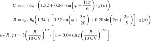
where \(\kappa_{0} = 2 \cdot 10^{22}~\mathrm{cm}^{2}\,\mathrm{s}^{ - 1}, \kappa_{1}(r) = 1 + 0.5\frac{r}{r_{0}}, r\) is the radial distance, r 0=100 AU is the size of the modulation region, and \(\kappa_{2}(R,\varphi) = A( \frac{R}{1\mathrm{0~\mathrm{GV}}} )^{\alpha } \cdot[ 1 + \mu\sin\varphi( \frac{R}{10~\mathrm{GV}} )^{\gamma } ]\). The term \(A( \frac{R}{10~\mathrm{GV}} )^{\alpha }\) describes the dependence of the 11-year variation of the GCR intensity on the rigidity R (Alania, Iskra, and Siluszyk 2008), which is the background state for the 27-day variation of the GCR intensity. The term \([ 1 + \mu\sin\varphi( \frac{R}{10~\mathrm{GV}} )^{\gamma } ]\) represents the dependence of the 27-day variation of the GCR intensity as a function of the rigidity R. The values of coefficients A,α,μ, and γ are specified based on the experimental results (Gil and Alania 2010) and on our assumptions for different epochs of SA. The solar wind velocity U, strength B of the IMF according to in situ measurements, and κ 2(R,φ) have the following expressions.
-
I.
In maximum epoch of SA:
 (2)
(2) -
II.
In the moderate epoch of SA:
 (3)
(3) -
III.
In the minimum epoch of SA:
 (4)
(4)Here U 0=400 km s−1, B 0=5.6 nT, and g(ρ)=eρ(0.01−ρ)/0.001 in Equations (2) – (4).


The pairs of constants (r 1,r 2),(r 3,r 4), and (r 5,r 6) are correlation coefficients between the 27-day variation of the GCR intensity on the one hand, and the 27-day variations of the solar wind velocity (r 1,r 3,r 5), and IMF (r 2,r 4,r 6) on the other, for three different SA epochs. The values of the correlation coefficients r 1,…,r 6 are presented in Table 2; they are the weights used in Equations (2) – (4). The justification of this procedure comes from the following motivation: For the period of analyses (23 October – 18 November 1991, 10 July – 5 August 1994, and 11 July – 6 August 1997), only the solar wind velocity and IMF strength showed relatively explicit quasi 27-day variations. Thus, as a whole, it is natural to ascribe the 27-day variation of the GCR intensity to the changes in these parameters. Our approach is not unusual in solving problems like the present case, when it is not possible to identify explicit causes and effects. Of course, under such circumstances the degree of compatibility between the theoretical results of modeling of the 27-day variation of the GCR intensity and the experimental data of neutron monitors is critical. We show below that this assumption is duly justified.
In order to find a numerical solution, Equation (1) is reduced to a dimensionless form:

where the coefficients A 1,A 2,…,A 12 are functions of spherical coordinates (ρ,θ,φ),t, and R,ρ=r/r 0 is the dimensionless distance, and \(n = \tfrac{n_{R}}{n_{0R}}\) is the relative density of the GCR particles for a given rigidity R. Here n R =4πR 2 f(R) is the density and f(R) is the directional average of the distribution function of GCR particles in the interplanetary space in terms of R. Similarly we define n=0R=4πR 2 f 0(R) for GCR particles in the interstellar medium. The intensity I 0 of the GCR particles in the interstellar medium (I 0=R 2 f 0) is taken from Webber and Lockwood (2001) and Caballero-Lopez and Moraal (2004) as \(I = \frac{21.1T^{ - 2.8}}{1 + 5.85T^{ - 1.22} + 1.18T^{ - 2.54}}\), where T is the particle’s kinetic energy.
Equation (5) has been transformed to a set of finite difference equations (e.g. Press et al. 2002), and the resulting system of algebraic equations was solved using the Gauss–Seidel iteration method (e.g. Kincaid and Cheney 2009). The solutions were found for a two-dimensional IMF (the latitudinal component of the IMF, B θ =0). In our model we consider changes during one solar rotation. Therefore the distribution of the GCR density is determined by the time-independent parameters, and thus the stationary state can be considered, i.e. A 12=0 in Equation (5).
As mentioned above, we used in situ measurements of the solar wind velocity and IMF strength as sources of the 27-day variation of the GCR intensity. Thus, it is necessary to have data implementation in the code. For this purpose we use the trigonometric approximation to get an analytic formula for those experimental data. Figures 7a – 7f show comparisons of experimental data (dots) with trigonometric approximations (solid curves) described by Equations (2) – (4). The correlation coefficients between those data sets are presented in Table 3. The solutions to the transport equation at Earth orbit (at 1 AU) in the equatorial region (θ=90∘) are presented in Figures 8 and 9. Figure 8 shows that the expected rigidity spectrum of the 27-day variation of the GCR intensity in the maximum epoch of SA is harder than in the minimum epoch. The values of γ are 0.59±0.08 (Figure 8a), 0.79±0.01 (Figure 8b), and 0.98±0.01 (Figure 8c) in the maximum, intermediate, and minimum epochs. These expected values of γ are reasonably compatible with the results obtained by using the experimental data from neutron monitors (Gil and Alania, 2010, 2011). Furthermore, an additional argument is given in Figure 9, which shows that the experimental data of the 27-day variation of the GCR intensity (daily measured values, squares) are in good agreement with the modeling results (relative density of the GCR particles n as a function of φ, solid curve) in the maximum (a), intermediate (b), and minimum (c) epochs of SA.

Comparison between experimental data (dots) and trigonometric approximation (solid curve) of the IMF strength (a, c, e) and solar wind velocity (b, d, f) in the maximum (a, b), intermediate (c, d), and minimum (e, f) epochs of SA, respectively.

Changes in the spectrum of the amplitudes of the 27-day variation of the GCR intensity in the maximum (a), moderate (b), and minimum (c) epochs of SA, respectively, at the Earth orbit.

Comparison between experimental data (the GCR intensity I [%] by Kiel NM, squares) and the modeling results (relative density n of GCR particles as a function of φ, solid curve) in the maximum (a), intermediate (b), and minimum (c) epochs of solar activity, respectively, at the orbit of the Earth.
Therefore, we may claim that our approach to use the correlation coefficients between the 27-day variation of the GCR intensity on the one hand, and the 27-day variations of solar wind velocity and IMF on the other, for different epochs of SA as the weight values in Equations (2) – (4), is successful. The values of the power-law exponent γ and amplitudes of the 27-day variation of the GCR intensity expected from the modeling and those obtained from the experimental data from neutron monitors are compatible within the accuracy of our calculations (Figures 8 and 9).
4 Conclusions
We show that the relative amplitude in rigidity spectrum, δD(R)/D(R)∝R −γ of all the three harmonics of the 27-day variation of the GCR intensity is hard in the maximum epochs and soft in the minimum epochs of SA for the period of 1965 – 2009 (see Table 1). We present the 3-D theoretical model of the 27-day variation of the GCR intensity for the maximum, intermediate, and minimum epochs of SA by implementing in situ measurements of the longitudinal changes of the solar wind velocity and IMF strength. The presented 3-D model is suitable to explain the experimental results; the expected rigidity spectrum of the 27-day variation of the GCR intensity is hard (γ=0.59±0.08) in the maximum epoch and soft (γ=0.98±0.01) in the minimum epoch of SA.
References
Ahluwalia, H.S., Fikani, M.M.: 2007, J. Geophys. Res. 112, A08105.
Alania, M.V.: 1978, In: Khantadze, A.G. (ed.) Proc. Inst. Geophys. 43, Georgian Academy of Sciences, Tbilisi, 5 – 14. (In Russian).
Alania, M.V.: 2002, Acta Phys. Pol. B 33, 1149 – 1166.
Alania, M.V., Dzhapiashvili, T.V.: 1979, In: Miyake, S. (ed.) Proc. 16th Int. Cosmic Ray Conf. 3. Institute for Cosmic Ray Research, University of Tokyo, Tokyo, 19 – 24.
Alania, M.V., Iskra, K., Siluszyk, M.: 2008, Adv. Space Res. 41, 267 – 274.
Alania, M.V., Gil, A., Iskra, K., Modzelewska, R.: 2005, In: Acharya, B.S., Gupta, S., Jagadeesan, P., Jain, A., Karthikeyan, S., Morris, S., Tonwar, S. (eds.) Proc. 29th Int. Cosmic Ray Conf. 2, Tata Institute of Fundamental Research, Mumbai, 215 – 218.
Caballero-Lopez, R.A., Moraal, H.: 2004, J. Geophys. Res. 109, A01101.
Dorman, L.I.: 1974, Cosmic Rays: Variation and Space Exploration, North-Holland, Amsterdam, 252 – 356.
Gil, A., Alania, M.V.: 2010, Adv. Space Res. 45, 429 – 436.
Gil, A., Alania, M.V.: 2011, J. Atmos. Solar-Terr. Phys. 73, 294 – 299.
Gil, A., Modzelewska, R., Alania, M.V.: 2012, Adv. Space Res. 50, 712 – 715.
Gil, A., Iskra, K., Modzelewska, R., Alania, M.V.: 2005, Adv. Space Res. 35, 687 – 690.
Jokipii, J.R., Kopriva, D.A.: 1979, Astrophys. J. 234, 384 – 392.
Jokipii, J.R., Levy, E.H., Hubbard, W.B.: 1977, Astrophys. J. 213, 861 – 868.
Kincaid, D.R., Cheney, E.W.: 2009, Numerical Analysis: Mathematics of Scientific Computing, American Mathematical Society, Providence, 216 – 218.
Leske, R.A., Cummings, A.C., Mewaldt, R.A., Stone, E.C.: 2011, Space Sci. Rev. doi: 10.1007/s11214-011-9772-1 , in press.
Parker, E.N.: 1965, Planet. Space Sci. 13, 9 – 32.
Press, W.H., Teukolsky, S.A., Vetterling, W.T., Flannery, B.P.: 2002, Numerical Recipes in C: The Art of Scientific Computing, Cambridge University Press, Cambridge, 830 – 856.
Smith, E.J.: 2011, J. Atmos. Solar-Terr. Phys. 73, 277 – 289.
Vernova, E.S., Tyasto, M.I., Baranov, D.G., Alania, M.V., Gil, A.: 2003, Adv. Space Res. 32, 621 – 626.
Wawrzynczak, A., Alania, M.V.: 2008, Adv. Space Res. 41, 325 – 334.
Wawrzynczak, A., Alania, M.V.: 2010, Adv. Space Res. 45, 622 – 631.
Webber, W.R., Lockwood, J.A.: 2001, J. Geophys. Res. 106, 29323 – 29332.
Yasue, S., Mori, S., Sakakibara, S., Nagashima, K.: 1982, Rep. Cosmic Ray Res. Lab., 7, Nagoya University, 1 – 225.
Acknowledgements
The referee helped us to improve our paper by valuable remarks and suggestions. The authors are grateful to the investigators of Kiel and Rome neutron monitors, and for use of the OMNIWeb data base.
Author information
Authors and Affiliations
Corresponding author
Rights and permissions
Open Access This article is distributed under the terms of the Creative Commons Attribution License which permits any use, distribution, and reproduction in any medium, provided the original author(s) and the source are credited.
About this article
Cite this article
Gil, A., Alania, M.V. Theoretical and Experimental Studies of the Rigidity Spectrum of the 27-Day Variation of the Galactic Cosmic Ray Intensity in Different Epochs of Solar Activity. Sol Phys 283, 565–578 (2013). https://doi.org/10.1007/s11207-012-0204-5
Received:
Accepted:
Published:
Issue Date:
DOI: https://doi.org/10.1007/s11207-012-0204-5