
Abstract
As quantum computation grows, the number of qubits involved in a given quantum computer increases. But due to the physical limitations in the number of qubits of a single quantum device, the computation should be performed in a distributed system. In this paper, a new model of quantum computation based on the matrix representation of quantum circuits is proposed. Then, using this model, we propose a novel approach for reducing the number of teleportations in a distributed quantum circuit. The proposed method consists of two phases: the pre-processing phase and the optimization phase. In the pre-processing phase, it considers the bi-partitioning of quantum circuits by Non-Dominated Sorting Genetic Algorithm (NSGA-III) to minimize the number of global gates and to distribute the quantum circuit into two balanced parts with equal number of qubits and minimum number of global gates. In the optimization phase, two heuristics named Heuristic I and Heuristic II are proposed to optimize the number of teleportations according to the partitioning obtained from the pre-processing phase. Finally, the proposed approach is evaluated on many benchmark quantum circuits. The results of these evaluations show an average of 22.16% improvement in the teleportation cost of the proposed approach compared to the existing works in the literature.
1 Introduction
Nowadays, quantum computation has become one of the interesting fields of computation and outperforms classical computation in certain algorithms [1,2,3,4]. In recent decades, rapid growth of science and engineering of quantum devices has led to advancement of quantum computation from exploration on single isolated quantum devices toward the appearance of multiqubit processors [5]. Quantum computations have many advantages over classical ones, but having a quantum system with many qubits and large-scale quantum device involves many implementation constraints. Unfortunately, interactions of qubits with the outside world lead to noise or decoherence [6, 7] and by increasing the number of qubits, the quantum information becomes delicate and fragile. It is also not a feasible solution to isolate qubits from the surrounding, because the qubits must be manipulated to achieve the required communication and computing, such as reading or writing operations. However, physical implementations like systems of trapped atomic ions can be accurately controlled and manipulated and a large variety of interactions can be engineered with high precision and measurements of relevant observables can be obtained with nearly 100% efficiency [8, 9].
Moreover, protecting the quantum information embedded in a qubit becomes harder by increasing the number of qubits. To overcome these limitations, it is reasonable to build a set of limited-capacity quantum computers with fewer qubits which are connected via a quantum or classical channel and can represent the behavior of whole monolithic quantum system. This concept is known as Distributed Quantum Computation (DQC). A DQC consists of smaller quantum circuits with limited capacity, located far from each other [10, 11].
Nowadays, superconducting qubit modality has been used to demonstrate prototype algorithms in the noisy quantum channel to have non-error-corrected qubit in quantum algorithm and are currently one of the approaches for realizing quantum devices and quantum coherence interaction with low noise and high controllability to implement medium and large quantum systems [12, 13]. Another technology to have a large-scale quantum system is photonic quantum computing. Quantum entanglement, teleportation, and quantum key distribution are used from this technology because photons present a quantum system with low noise and high performance [14].
In recent years, there have been many attentions toward DQC. There are two important reasons for these special attentions: first to have a quantum network for creating the infrastructure of a quantum internet and second to scale up the quantum systems.
In order to perform a distributed quantum computation, it is necessary for a protocol to transmit quantum information from one quantum system to another. Long-distance quantum communication is a technological challenge for the physical realizations of quantum communication [15]. In this regard, teleportation [16] is an elementary protocol to distribute the entangled qubits and using this protocol, quantum information can be distributed through quantum links and quantum systems.
The main idea of teleportation is the transformation of qubit states from one location to another without physically moving them [17]. According to no-cloning theorem [18], when a qubit is teleported to a subsystem, it cannot be used in own subsystem and it is required to be returned back in order to be used in its home subsystem. This protocol is an expensive operation in DQC whose number should be minimized.
As shown in Fig. 1, any number of contiguous global CNOT gates that act on the same qubit, can be executed by one teleportation. In this figure, two contagious global CNOT can be executed by teleporting \({q}_{1}\) from \({P}_{1}\) to \({P}_{2}\). Then by executing these gates, q1 is teleported back to its own partition. This concept is used in the optimization phase of our work. By using the commutativity property of quantum gates, it is tried to exchange gates, so that the gates with common qubit are located adjacent to each other. By this operation, the number of required teleportations is reduced.

A group of global CNOT gates that act on the same qubit can be executed by one teleportation
In this paper, we propose a new matrix model for representing quantum circuits which is called connectivity matrix model of quantum circuits or CMMQC. Based on this model, a new algorithm is presented to minimize the teleportation cost. The algorithm consists of two steps: the pre-processing phase and the optimization phase. The pre-processing phase distributes the quantum circuit into two (or more) balanced partitions aiming to minimize the number of circuit cuts or global CNOT gate. After partitioning the quantum circuit, some gates become global gate and their control and target qubits are placed in different partitions. Execution of these global gates requires that one of the qubits to which they are applied, is teleported from its home partition to the destination partition where the gate is executed and then to go back to the home partition. Qubit migration from one subsystem to another through teleportation imposes cost to the distributed quantum circuit. So, NSGA-III algorithm is used to partition the quantum circuit into two balanced partitions to minimize the number of global gates. In the next phase, two heuristics are applied to the partitioning obtained from the previous step in order to minimize the required number of teleportations.
In Sect. 2, we introduce the related work of DQC. Our novel connectivity matrix model of quantum circuits (CMMQC) is introduced in Sect. 3. Then in Sect. 4, we propose a new approach for optimizing the number of teleportations in the distributed quantum circuit using CMMQC. Finally, we evaluate our approach on several standard quantum circuits in Sect. 5.
2 Related work
First idea for a distributed quantum computing was suggested by Grover [2], Cleve and Buhrman [19] and later Cirac et.al. [20]. Grover presented a distributed quantum system consisting of several subsystems located on separate locations. These subsystems performed their computations and forwarded their output to a base station when necessary. Grover showed that the computation time is proportional to the number of subsystems of the distributed system.
Recently, DQC have been used in many applications. In [21], the authors considered two black boxes as two quantum devices and these devices were prevented from communicating with each other and designed a trusted quantum cryptography to share a random key with security based on quantum physics.
A practical application for quantum machine learning (QML) was proposed in [22]. In this application, a distributed secure quantum machine learning was considered for classical client to delegate a remote quantum machine learning to quantum server with data privacy.
There are many limitations for realizing a quantum computer. As mentioned above, building a monolithic quantum system with many qubits has some technical limitations and these limitations lead to the development of distributed quantum computing. In [23], an architecture for distributed quantum computing with two types of communication was presented: Type I and Type II. In Type I, the quantum systems use the quantum link to communicate between subsystems and in Type II, classical communication is used between subsystems. By using this definition, our distributed quantum system is type I.
Beals et.al [24] showed that a quantum system can be distributed to some nodes connected by a hypercube graph in a distributed quantum computer which imitates a quantum circuit with low overhead. Cuomo et.al [25] considered the main challenges and open problems in the distributed quantum computing. They introduced the concept of quantum internet which is the essential infrastructure of distributed quantum computing ecosystem. They presented a bottom-up approach including set of layers that altogether provide the ecosystem of distributed quantum computing. The challenges of designing quantum internet were considered in [26]. They showed that faster processing speed is achieved by connecting quantum computers via quantum internet. In another work from Caleffi et.al [27], the authors studied the creation of quantum internet and considered teleportation as the main protocol to transfer the information. Then they explored the challenges in the design of quantum internet. Recently, imperfect entanglement for non-local quantum operations and the effect on the fidelity for a distributed implementation of a quantum phase estimation circuit has been considered in [28]. The authors have only considered imperfect entanglement (i.e., fidelity < 1). All local operations were assumed perfect and qubits were assumed not to decohere.
Zomorodi et al. [29], presented a procedure to minimize the number of communications required in a distributed quantum circuit (DQC) in terms of the number of teleportations. They considered a system consisting of two separated subsystems and have located far from each other. Different configurations for executing each non-local gate were considered and for each of them, the proposed method was run to find the minimum number of teleportations with exponential complexity. Genetic algorithm was used in [30] to find the minimum number of communication between two partitions in a distributed quantum system and the optimization problem was solved in a more effective way and less complexity. The authors of [10] also presented an automated method to distribute a quantum circuit into some partitions in such a way that teleportation cost minimized. They reduced the problem of quantum circuit distribution to hyper graph partitioning problem by mapping quantum circuits to hypergraphs. In their approach, first the qubits and CZ gates of a quantum circuit were mapped to nodes and hyper edges of a hyper graph, respectively. Then this hypergraph was partitioned using third party solvers.
A dynamic programming approach to distribute the quantum circuit into K parts was proposed in [31]. In this approach, first the quantum circuit was converted into a bi-partite graph and then the gates and qubits are placed in each part of the graph. Then by applying a dynamic programming approach, this graph was partitioned into K parts with the aim to minimize the number of global gates. The authors in [32] also have discussed the issue of reducing the communication cost in a distributed quantum circuit composed of up to three-qubit gates and have presented a new heuristic method to solve it.
In another work [33], the authors presented an efficient partitioning approach to minimize the communication cost. They combined both gate and qubit teleportation concepts to minimize the number of teleportations. They proposed a hybrid partitioning approach called WQCP, which combines both teledata and telegate ideas.
3 Matrix model of quantum computation
Our proposed model is based on a new matrix representation of quantum circuits. For the first time, we are defining a connectivity matrix representation model of quantum circuits called CMMQC which consists of the following elements:
-
As input it takes a quantum computation in the circuit model named QC with n qubits \(Q=\left\{{q}_{1}, {q}_{2},\dots ,{q}_{n}\right\}\) numbered sequentially.
-
A gate set \(\mathcal{G}=\{{g}_{1},{g}_{2},\dots ,{g}_{m}\}\) with m gates, where each gate has at most two qubits associated with it (gates with more than two qubits are decomposed to one and two qubit gates before they are mapped into the new model [34]).
-
A gate library \(\mathcal{U}\). Our gate library is \(\mathcal{U}=\left\{X, CNOT, H,Y,Z\right\}\). This gate set is universal and all the gates in \(\mathcal{U}\) have some efficient physical implementations associated with them [35].
-
Single-qubit gates\(g(t,{q}_{s}\)) and two-qubit gates \(g(t,{q}_{c},{q}_{t})\) in the set \(\mathcal{G}\) have two and three parameters, respectively.\(t\) is the execution time in terms of the time step of the sequential execution of the gate in the quantum circuit. For single-qubit gate \(g\left(t,{q}_{s}\right),\) \({q}_{s}\) is the index of the input qubit of the gate and for two-qubit gate \(g(t,{q}_{c},{q}_{t}) ,\) \({q}_{c}\) and \({q}_{t}\) are the index of the control and target qubits associated with that gate, respectively. The index of the qubit is the number assigned to it by the quantum circuit model. In the quantum circuit model, qubits are numbered from top to button starting by 0 to the number of the qubits minus one\((n-1)\).
The quantum circuit defined in this manner is processed as follows to create the connectivity matrix called CM. This matrix is a two-dimensional data structure which shows the existence of connectivity between gates and qubits in scheduled time steps that form the quantum computation in a sequence defined by the scheduler; i.e., quantum circuit scheduling algorithm.
The formation of the connectivity matrix is defined by the following rules:
-
The rows and columns of this matrix represent the qubits and gates, respectively.
-
The order by which qubits and gates are placed on the rows and columns of this matrix is specified by the quantum circuit model of the quantum computer.
-
The elements of the \(n\times m\) connectivity matrix \(CM\) are defined as follows:
-
$$ {\text{CM}}\left[ {{q_{\text{c}}}} \right]\left[ t \right] = 1,CM\left[ {{q_t}} \right]\left[ t \right] = 2;\quad \forall \;g\left( {t,{q_{\text{c}}},{q_t}} \right),\;\quad 1 \leqslant t \leqslant m;$$
-
$$ {\text{CM}}\left[ {{q_{\text{s}}}} \right]\left[ t \right] = - 1;\quad \forall \;g\left( {t,{q_{\text{s}}}} \right),\;\quad \;1 \leqslant t \leqslant m; $$
-
$$ {\text{CM}}\left[ i \right]\left[ t \right] = 0;\quad {\text{otherwise}},\quad 1 \leqslant i \leqslant n; $$
-
As an example, Fig. 2 represents the connectivity matrix (CM) of a sample quantum circuit with three qubits and six gates.

A quantum circuits and its connectivity matrix
The values presented in the connectivity matrix are arbitrarily selected to distinguish between different gate types. For example, Fig. 2 shows a quantum circuit and its connectivity matrix with 3 qubits and 6 gates.
4 Distributed quantum circuit optimization
Using the connectivity matrix, now we describe our approach for distributed quantum circuit optimization. First, we consider the quantum circuit scheduling which is required for constructing the connectivity matrix. The columns of the connectivity matrix are the scheduled quantum gates. The following rules are held in the scheduling of the quantum circuit:
-
1.
Each qubit can be used by just one quantum gate at a given time step.
-
2.
In the presence of logical dependency between quantum gates, they should be executed in order. It implies the non-commutativity property between some gates.
Commutativity between quantum gates is an important part of our proposed approach. Let us consider two gates \(CNOT({t}_{1},{q}_{{c}_{1}},{q}_{{t}_{1}})\) and \(CNOT({t}_{2},{q}_{{c}_{2}},{q}_{{t}_{2}})\). These gates commute if they have one of the following properties:
-
Their control qubits \({q}_{{c}_{1}}\) and \({q}_{{c}_{2}}\) be the same.
-
They have no common qubits.
Now in the following, we describe our main algorithm for reduction in teleportation cost which consists of two phases: pre-processing phase and optimization phase. We will describe these phases as following.
4.1 Pre-processing phase
In this phase, the quantum circuit is distributed into two partitions. By partitioning the quantum circuit, every single-qubit gate can be executed locally in each partition without communications. In contrast, some CNOT gates become global and their target and control qubits belong to different partitions so that two teleportations are required for executing each of them. Therefore, minimizing the number of global gates is considered in this phase. To increase the performance of each partition, we will impose a load balancing requirement: the number of qubits in each partition must be almost equal.
This problem can be considered as a multi-objective problem which is well-known as an NP-hard problem [36]. In our problem, bi-partitioning is proposed. Two objectives for the distribution of the quantum circuit into two partitions are considered:
We considered this problem as a multi-objective optimization problem (MOP). Many algorithms have been proposed to solve MOPs such as [37, 38]. NSGA-III is one of the most popular multi objective optimization algorithms [39]. Generally, NSGA-III has the following parts: Population initialization and encoding, Non-Dominated sorting, crowding, selection, genetic operators, recombination and selection.
Encoding in the first step of NSGA-III, the encoding mechanism for representing chromosomes is required. In this study, the algorithm uses a chromosome with \(n+1\) genes where n is the number of qubits. The value of \({\left(i+1\right)}^{th}\) genes corresponds to the \({i}^{th}\) qubit and indicates the position of \({i}^{th}\) qubit in the circuit. The parameter \(cutline\) is considered as a qubit position in the circuit model, where after that the qubits are located in Partition II. The value of the first gene indicates the value of cutline and means that \((cutline )\) genes are located in Partition I and\((n-cutline\)) qubits are located in Partition II. This structure has been shown in Fig. 3.

Instruction of chromosome for NSGA-III
For example, Fig. 4 represents how a chromosome is mapped into a quantum circuit. A sample chromosome is shown in Fig. 4a. As shown in this figure, the first gene of this chromosome represents the cutline locates between Lines 2 and 3 in the circuit and Partitions I and II consist of 2 and 4 qubits, respectively. \({q}_{1}\) is transferred to Line 3 and other qubits are transferred to Lines 1, 2, 5, 6, 4 according to the chromosome, respectively. The primary circuit has been shown in Fig. 4b. The algorithm provides the circuit of Fig. 4c by assigning each gene to its position. In this example,\(GlobalNum\) and \(QNum\) are 8, 2, respectively.

a A sample chromosome, b primary quantum circuit, c partitioned quantum circuit obtained from the sample chromosome in a
Non-dominated sorting In NSGA-III, to calculate the rank of each chromosome, they are sorted into different non domination levels by procedure proposed by Kalyanmoy [40].
After applying NSGA-III to the quantum circuit, it is partitioned into two balanced parts with equal number of qubits. Figure 5 shows the optimized chromosome (Fig. 5a), distributed quantum circuit (Fig. 5b), connectivity matrix before pre-processing (Fig. 5c) and after pre-processing phase (Fig. 5d) for the circuit of Fig. 4b. As shown in this figure, qubits 1, 4 and 6 are located in Partition I and the other ones are located in Partition II. The GlobalNum and QNum are obtained as 4 and 0, respectively.

The optimized quantum circuit of Fig. 4 after pre-processing phase
4.2 Optimization phase
In the pre-processing phase, the quantum circuit was distributed into two partitions so that the resulting distributed quantum circuit had the minimum number of global gates compared to other distributions.
Based on the result of the pre-processing phase, qubits are distributed in two quantum subsystems. To execute each non-local CNOT gate, one of its two qubits should be teleported from its home partition to another partition. This qubit is called migrated qubit and can be used in the destination partition as long as possible and then it is teleported back to the home partition. By this schema the number of required teleportation is minimized. In other words, any number of sequential CNOT gates that operate on the same control qubit and whose target qubits belong to the same partition, can be executed by one teleportation instead of a number of teleportations. Therefore, after this phase two heuristic algorithms are proposed for teleportation called Heuristic I and II. They are applied to the optimized circuit generated from the pre-processing phase. These heuristics are described as following:
4.2.1 Heuristic I
As stated, using the connectivity matrix created in the pre-processing phase the quantum circuit is distributed into two balanced partitions. In Heuristic I, when a qubit belonging to a global gate is teleported to the other partition, i.e., migrated qubit, it may be used by other gates as long as possible without the need to be teleported back. This means that the migrated qubit has been used optimally and the adjacent and consecutive global gates with common qubit are executed by one teleportation.
This heuristic tracks the whole connectivity matrix. For each gate \({g}_{i}\), a list of gates called \({DispList}_{i}\) which can commute with \({g}_{i}\) is obtained. In the next step, each gate of this list commutes with \({g}_{i}\) and the number of teleportations is calculated for this condition. Condition with the smallest number of teleportations is found and the connectivity matrix is updated. This step is repeated for all gates and finally the order of gates with the minimum number of teleportations is reported. The pseudo code for Heuristic I is given in Algorithm 1.
This algorithm takes as input the obtained partitioning of the pre-processing phase and reports a connectivity matrix with minimum number of teleportations. At the first line of the algorithm, Function ConnectivityMatrix constructs the connectivity matrix of quantum circuit and puts it in Matrix TCM. In Line 2, the Function TeleportationNum sets variable Mintel to the minimum required number of teleportations of circuit. As stated, each column of the connectivity matrix represents one gate. In Lines (3–7), for each Column i of TCM, list of all possible columns which can commute with Column \(i\) is created. This list is called \({DispList}_{i}\) and is created in Lines 3–7 of the algorithm. In Lines 8–15, each gate \({g}_{i}\) commutes with each of its corresponding members of \({DispList}_{i}\) and the circuit is updated by Function UpdateCircuit in Line 10 and its corresponding connectivity matrix and number of teleportations are stored in Matrix \(TempCM\) and \(TempTelNum\), respectively. If the number of teleportations in updated circuit is less than \(MinTel\), then TCM and \(MinTel\) are updated by new change (Lines 12–14). These steps are repeated for all of the columns in the connectivity matrix.

For example, a circuit with 6 qubits and 4 gates is given in Fig. 6a. At the beginning of the algorithm, MinTel is 8. In this circuit \({DispList}_{1}\) is \(\left\{{g}_{2},{g}_{3}\right\}\). Then \({g}_{1}\) commutes with \({g}_{2}\) (Fig. 6b). By this commute, the number of teleportations is 8 and the circuit is not changed. Finally, \({g}_{1}\) commutes with \({g}_{3}\) in Fig. 6c. By this commute, the number of teleportations will be 4 at the end (Fig. 6c). This is because by teleporting qubit \({q}_{2}\) from \({P}_{1}\) to \({P}_{2}\), two gates \({g}_{3}\) and \({g}_{2}\) are consecutive and can be executed by one teleportation. Then \({q}_{2}\) is teleported back to \({P}_{1}\). Finally, by teleporting \({q}_{1}\) from \({P}_{1}\) to \({P}_{2}\), two gates \({g}_{1}\) and \({g}_{4}\) become consecutive and can be executed by one teleportation. Therefore, two teleportations is required for executing the circuit in Fig. 6c and also two more teleportations are required to return the teleported qubits back to their home partition and so the final number of teleportations is doubled and in this example the optimum number of teleportations is equal to 4.

An example of Heuristic I
4.2.2 Heuristic II
In this section, another heuristic is proposed. In this heuristic, each column i is compared to its adjacent columns \(\left(i+1 and i-1\right)\). Two adjacent columns have three different configurations as following:
-
1.
Composition state if two consecutive values of ‘1’ are found in rows of the connectivity matrix, columns corresponding to them are merged together. The same is performed for two consecutive ‘2’s or two consecutive ‘-1’s. It means that two consecutive gates consist of common target qubit or common control qubit and can be merged. This condition is formulated as follows:
$$ \forall \;0 \leqslant j \leqslant m\quad {\text{if}}\;\;{\text{CM}}\left[ i \right]\left[ j \right] = {\text{CM}}\left[ i \right]\left[ {j + 1} \right] $$$$ \Rightarrow {\text{CM}}\left[ i \right]\left[ j \right] = \max \left( {{\text{CM}}\left[ i \right]\left[ j \right],\;CM\left[ i \right]\left[ {j + 1} \right]} \right)\& \,\;{\text{remove}}\,{\text{column\;}}\,j + 1$$ -
2.
Block state: if patterns ‘1, 2’ or ‘2, 1’ are found in two consecutive columns of the connectivity matrix, then two columns are merged together and values ‘3’ or ‘4’ are placed in the position of common qubit for patterns ‘1, 2’ or ‘2, 1,’ respectively. It means that in two consecutive CNOT gates, the index of the target qubit of one gate is equal to the index of the control qubit of another gate or vice versa. This condition is formulated as one of following cases:
-
(a)
$$ \begin{gathered} \forall \;0 \leqslant j \leqslant m\;\quad {\text{\;if}}\;\left( {{\text{CM}}\left[ i \right]\left[ j \right] = 1\;\& \;{\text{CM}}\left[ i \right]\left[ {j + 1} \right] = 2} \right) \hfill \\ \quad \Rightarrow {\text{CM}}\left[ i \right]\left[ k \right] = \left\{ {\begin{array}{*{20}{c}} {3\quad k = j\;} \\ {{\text{max}}\left( {{\text{CM}}\left[ i \right]\left[ j \right]\;,\;CM\left[ i \right]\left[ {j + 1} \right]} \right)\;\quad {\text{otherwise}}\,{\text{and}}\,{\text{remove}}\,{\text{column\;}}\,j + 1\;} \end{array}} \right. \hfill \\ \end{gathered} $$
-
(b)
$$ \begin{gathered} \forall \;0 \leqslant j \leqslant m\quad {\text{if}}\;\;\left( {{\text{CM}}\left[ i \right]\left[ j \right] = 2\,\& \;{\text{CM}}\left[ i \right]\left[ {j + 1} \right] = 1} \right) \hfill \\ \quad \Rightarrow {\text{CM}}\left[ i \right]\left[ k \right] = \left\{ {\begin{array}{*{20}{c}} {4\quad k = j\;} \\ {{\text{max}}\left( {{\text{CM}}\left[ i \right]\left[ j \right],\,{\text{CM}}\left[ i \right]\left[ {j + 1} \right]} \right)\,{\text{otherwise}}\,{\text{and}}\,{\text{remove}}\,{\text{column\;}}\,j + 1\;} \end{array}} \right. \hfill \\ \end{gathered} $$
-
(a)
-
3.
Figure 7 depicts these three conditions. In Fig. 7a, two consecutive ‘1’s are found in Row 1. In other words, two consecutive gates \({g}_{i}\) and \({g}_{i+1}\) have common control qubits and State (A) has accrued. Columns \(i\) and \(i+1\) are merged and connectivity matrix is updated according to Fig. 7a. In Fig. 7b, State (B) has been shown. In this figure, Pattern ‘1, 2’ has been found and the connectivity matrix is updated. Commutativity state (C) is shown in Fig. 7c.
Fig. 7 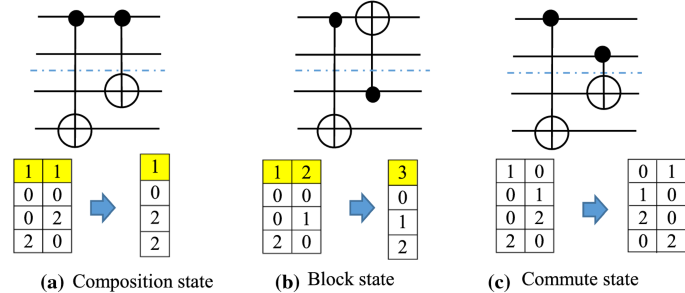
Three states: a, b, c
-
3.
Commutativity state Two adjacent gates are independent and can commute with each other. In other words, these gates do not have any common qubit.

Algorithm 2 shows the pseudo-code of Heuristic II. This algorithm has quantum circuit as input and optimized connectivity matrix with minimum number of teleportations as output. At the first part of the algorithm, connectivity matrix of quantum circuit is calculated by Function ConnectivityMatrix and it is placed in a matrix called TCM. Then for each column of TCM, it is compared to its adjacent column in Lines 6–10 to find States (A), (B), or (C (. State (A) is considered in Line 6 and function Composition merges two columns. In Lines 8–9, State (B) is considered and function Block merges and updates the connectivity matrix. Commute state is checked in Line 10. Two columns commute if the number of columns of connectivity matrix is reduced by this movement. As mentioned above, States (A) and (B) reduce the length of the connectivity matrix. Lines 4–14 are repeated until the length of the connectivity matrix is not changed.

Lines 4–14 were performed to compare the Columns i and i + 1 for finding each states (A) to (C) forwardly. Also these states may accrue in comparison to Columns i and i-1. Therefore as same Lines 4–14, these steps are repeated from Last column down to column 0 to compare column i and i-1 to reduce size of connectivity matrix. Lines 4–24 are repeated until the length of the connectivity matrix is not changed.
For example, Fig. 8 shows the steps of Heuristic II on the optimized circuit of Fig. 4. The teleportation cost (TC) and the length of the connectivity matrix (L) are reported bellow each matrix. Also in each step, (F) or (B) indicate that direction is forward or backward. These steps are as follows:
-
In Column \(i=1\), two consecutive values "1" are found and Condition (A) has occurred. Columns 1 and 2 are merged.
-
For \(i=2\) none of the Conditions (A), (B), or (C) occurred. But in Column \(i=3\), there is a block condition and the connectivity matrix is updated.
-
In Column \(i=4\), if two Columns 4 and 5 commute, then column 5 and 6 have composition condition. Therefore, columns 4 and 5 commute.
-
In Column \(i=5\), two consecutive values of "-1" is found and there is a composition condition.
-
In Column \(i=6\), commute condition has happened.
-
There is a composition condition in Column 7.
-
Up to this point, the connectivity matrix was traced forwardly. When \(i\) reached to the last column, the steps mentioned above are repeated backward and Columns \(i\) and \(i-1\) are compared with each other to find one of the mentioned three conditions.

Steps of running Heuristic II on example circuit of Fig. 4
Compared to Heuristic I, the second heuristic has much less execution time. It is clear that the time complexity of the Heuristic I is \(O(({TCM.Length)}^{2})\) in which \((TCM.Length)\) is the number of columns of TCM. The time complexity of Heuristic II is equal to \(O(C\times \left|TCM\right|.Length)\) in which C is the number of iterations of while loop. In the best and worst cases, the number of iterations of while loop are constant value C and \((TCM.length)\), respectively. Therefore, the time complexity of Heuristic II is \(O(|TCM|)\) and \(O{(|TCM|)}^{2}\) in the best and worst cases, respectively.
5 Results and discussion
The proposed method was evaluated on different quantum circuits. The first set of benchmark circuits are from Revlib which contain reversible circuits and can be decomposed into elementary quantum gates [35]. The second one is from Quipper library. Quipper is implemented as an embedded language in Haskell, and has many high level features [41]. Two type of experiments were done to evaluate the proposed method:
-
The effect of pre-processing phase on minimizing the number of teleportations.
-
Execution time of Heuristic Algorithms 1 and 2.
Also, we compared proposed approach with methods of [29].
First, the effect of the pre-processing phase on some circuits was considered. Figure 9 shows the number of teleportations on different samples with and without the pre-processing phase. As shown in this figure, the pre-processing phase reduced the number of teleportations in three samples. Also Fig. 10 shows the overall overhead of applying the pre-processing phase on the whole execution time of algorithm.

Effect of pre-processing on teleportation cost

Effect of pre-processing on execution time
In the second experiment, the teleportation cost and the execution time of the Heuristic I and II are considered. The teleportation cost (TC), execution time (ET) and speed-up for two proposed heuristics are given for different quantum circuits in Table 1. By increasing the number of qubits, speed-up of Heuristic I was increased in comparison to Heuristic II. It means that by increasing the number of qubits, the execution time of heuristic I was more than heuristic II. Also, Fig. 11 shows the speed-up of Heuristics I in comparison to Heuristic II.

Speed-up of the heuristic II as compared to heuristic I algorithm
Also, the proposed Heuristics I and II were evaluated on different quantum circuits from RevLib and were compared to the random search (RS), and the methods of [20] and [29, 30] in Table 2. In this table, the teleportation cost and the execution times are reported for these methods. Moreover, in order to show the effectiveness of Heuristic II, the speed-up and the TC improvement (TC imp) of Heuristic II in comparison to the method of [30] were reported in this table. In the case of 4gt5_76, Sym9_147, and 4-qubit QFT benchmarks, TC has been improved and in other ones, TC improvement was 0%. Also Fig. 12 shows the speed-up (a) and the TC improvement (b) of Heuristic II in comparison to the proposed method of [30].

6 Conclusion
In this paper, a new connectivity matrix model was presented to distribute the quantum circuit into balanced partitions in order to minimize the number of teleportations required in a distributed quantum circuit. The proposed method consists of two phases. In the first phase, the quantum circuit is distributed into two balanced partitions. In this phase, two objective functions are considered to minimize: the number of global gates and the difference between numbers of qubits of partitions. A NSGA-III algorithm was proposed to solve this problem. The output of this phase is two balanced partitions with minimum number of global gates. In the second phase, two heuristic methods were proposed to minimize the required number of teleportations for the distributed circuit of previous phase. Finally, we compared the proposed approach by some approaches and the results showed a significant improvement as compared to the previous studies.
References
Grover, L.K.: A fast quantum mechanical algorithm for database search. In: Proceedings of the Twenty-Eighth Annual ACM Symposium on Theory of Computing (1996)
Grover, L.K.: Quantum Telecomputation (1997). arXiv preprint quant-ph/9704012
Shor, P.W.: Polynomial-time algorithms for prime factorization and discrete logarithms on a quantum computer. SIAM Rev. 41(2), 303–332 (1999)
Huang, H.-L., et al.: Experimental blind quantum computing for a classical client. 119(5), 050503 (2017)
Krantz, P., et al.: A quantum engineer's guide to superconducting qubits. 6(2), 021318 (2019)
Cacciapuoti, A.S., et al.: When entanglement meets classical communications: Quantum teleportation for the quantum Internet. IEEE Trans. Commun. (2020).
Cacciapuoti, A.S., Caleffi, M.: Toward the quantum Internet: A directional-dependent noise model for quantum signal processing. In: ICASSP 2019–2019 IEEE International Conference on Acoustics, Speech and Signal Processing (ICASSP). IEEE (2019)
Blatt, R., Roos, C.F.J.N.P.: Quantum simulations with trapped ions. 8(4), 277–284 (2012)
Bruzewicz, C.D., et al.: Trapped-ion quantum computing: progress and challenges. 6(2), 021314 (2019)
Andrés-Martínez, P., Heunen, C.: Automated distribution of quantum circuits via hypergraph partitioning. Phys. Rev. A 100(3), 032308 (2019)
Meter, R.v. and M. Oskin, : Architectural implications of quantum computing technologies. ACM J. Emerg. Technol. Comput. Syst. (JETC) 2(1), 31–63 (2006)
Kjaergaard, M., et al.: Superconducting qubits: current state of play. 11, 369–395 (2020)
Huang, H.-L., et al.: Superconducting quantum computing: a review. 63(8), 1–32 (2020)
Slussarenko, S., Pryde, G.J.J.A.P.R.: Photonic quantum information processing: a concise review. 6(4), 041303 (2019)
Brassard, G., et al.: Limitations on practical quantum cryptography. Phys. Rev. Lett. 85(6), 1330 (2000)
Bennett, C.H., et al.: Teleporting an unknown quantum state via dual classical and Einstein-Podolsky-Rosen channels. Phys. Rev. Lett. 70(13), 1895 (1993)
Meter, R.V., et al.: Arithmetic on a distributed-memory quantum multicomputer. ACM J. Emerg. Technol. Comput. Syst. (JETC) 3(4), 1–23 (2008)
Wootters, W.K., Zurek, W.H.: A single quantum cannot be cloned. Nature 299(5886), 802–803 (1982)
Cleve, R., Buhrman, H.: Substituting quantum entanglement for communication. Phys. Rev. A 56(2), 1201 (1997)
Cirac, J., et al.: Distributed quantum computation over noisy channels. Phys. Rev. A 59(6), 4249 (1999)
Reichardt, B.W., Unger, F., Vazirani, U.J.N.: Classical command of quantum systems. 496(7446), 456–460 (2013)
Sheng, Y.-B., Zhou, L.J.S.B.: Distributed secure quantum machine learning. 62(14), 1025–1029 (2017)
Yepez, J.: Type-II quantum computers. Int. J. Mod. Phys. C 12(09), 1273–1284 (2001)
Beals, R., et al.: Efficient distributed quantum computing. Proc. Roy. Soc. A Math. Phys. Eng. Sci. 469(2153), 20120686 (2013)
Cuomo, D., Caleffi, M., Cacciapuoti, A.S.: Towards a Distributed Quantum Computing Ecosystem. (2020). arXiv preprint arXiv:2002.11808
Caleffi, M., Cacciapuoti, A.S., Bianchi, G.: Quantum internet: from communication to distributed computing! In: Proceedings of the 5th ACM International Conference on Nanoscale Computing and Communication (2018)
Cacciapuoti, A.S., et al.: Quantum internet: networking challenges in distributed quantum computing. IEEE Netw. 34(1), 137–143 (2019)
Briegel, H.-J., et al.: Quantum repeaters: the role of imperfect local operations in quantum communication. Phys. Rev. Lett. 81(26), 5932 (1998)
Zomorodi-Moghadam, M., Houshmand, M., Houshmand, M.: Optimizing teleportation cost in distributed quantum circuits. Int. J. Theor. Phys. 57(3), 848–861 (2018)
Houshmand, M., Zahra, M., Zomorodi-Moghadam, M., Houshmand, M.: An evolutionary approach to optimizing teleportation cost in distributed quantum computation. Int. J. Theor. Phys. 59(4), 1315-1329 (2020)
Davarzani, Z., Zomorodi-Moghadam, M., Houshmand, M., Nouri-baygi, M.: A dynamic programming approach for distributing quantum circuits by bipartite graphs. Quantum Inf. Process. 19(10), 1-18 (2020)
Daei, O., Navi, K., Zomorodi-Moghadam, M.: Optimized quantum circuit partitioning. Int. J. Theor. Phys. 59(12), 3804-3820 (2020)
Nikahd, E., et al.: Automated window-based partitioning of quantum circuits. 96(3), 035102 (2021).
Marinescu, D.C.: Classical and Quantum Information. Academic Press (2011)
Barenco, A.: Elemntary gates for quntom computation. Phys. Rev. A Gen. Phys. 52(5), 3457–3467 (1995).
Andreev, K., Racke, H.: Balanced graph partitioning. Theory Comput. Syst. 39(6), 929–939 (2006)
Miettinen, K.: Nonlinear multiobjective optimization, vol. 12. Springer Science & Business Media (2012)
Deb, K.: Multi-objective optimization. In: Search Methodologies, pp. 403–449. Springer (2014)
Cui, Z., et al.: Improved NSGA-III with selection-and-elimination operator. Swarm Evol. Comput. 49, 23–33 (2019)
Deb, K., et al.: A fast and elitist multiobjective genetic algorithm: NSGA-II. 6(2): 182–197 (2002)
Alexander Green, P.L.L., Ross, N.J., Selinger, P., Va-liron, B.: An introduction to quantum proigramming in quipper. In: 5th International Conference on Reversible Computing, RC 2013. Springer. Victoria, British Colombia (2013).
Author information
Authors and Affiliations
Corresponding author
Additional information
Publisher's Note
Springer Nature remains neutral with regard to jurisdictional claims in published maps and institutional affiliations.
Rights and permissions
Open Access This article is licensed under a Creative Commons Attribution 4.0 International License, which permits use, sharing, adaptation, distribution and reproduction in any medium or format, as long as you give appropriate credit to the original author(s) and the source, provide a link to the Creative Commons licence, and indicate if changes were made. The images or other third party material in this article are included in the article's Creative Commons licence, unless indicated otherwise in a credit line to the material. If material is not included in the article's Creative Commons licence and your intended use is not permitted by statutory regulation or exceeds the permitted use, you will need to obtain permission directly from the copyright holder. To view a copy of this licence, visit http://creativecommons.org/licenses/by/4.0/.
About this article

Cite this article
Ghodsollahee, I., Davarzani, Z., Zomorodi, M. et al. Connectivity matrix model of quantum circuits and its application to distributed quantum circuit optimization. Quantum Inf Process 20, 235 (2021). https://doi.org/10.1007/s11128-021-03170-5
Received:
Accepted:
Published:
DOI: https://doi.org/10.1007/s11128-021-03170-5