On the problem of the purchasing power of money by A. A. Konüs and S. S. Byushgens: translation and commentary

Abstract

In 1939, Econometrica published an English translation of Konüs (1924). Since then, Konüs (1924 [1939]) has become a classic work on the theory of the cost of living index, inspiring many other studies in the field. On the other hand, very few scholars have had the opportunity to read another, equally important, work by Konüs (co-authored with Byushgens) published in 1926 by the same Institute. This other paper of Konüs also pioneered several fundamental concepts and results in economics (including duality theory, the theory of inverse demand functions and the theory of exact index numbers), yet somehow it appears that it has never been translated into English (or any other language). We bridge this gap by offering a translation and a commentary on this important paper.

1 Introduction

In 1939, Econometrica published an English translation of Konüs (1924), due to the efforts of Henry Schultz who also provided a discussion on that paper in the same issue of the journal (Schultz (1939)). In a nutshell, the famous paper of Konüs (1924) introduced the concept of a true cost of living index, C(u, p¹)/C(u, p⁰), as a ratio of expenditure or cost functions where the consumer’s utility level u is held constant in the numerator and denominator of the index but the current period price vector p¹ appears in the numerator and the base period price vector p⁰ appears in the denominator of the ratio. Eventually, this article of Konüs (1924 [1939]) became a classic and fundamental work on the theory of the cost of living index, and on index numbers in general, inspiring many other works. Realizing the importance of his paper, in a footnote of the paper, the Editor noted:

“We are very glad to present in full this excellent work which so far has been known to most econometricians only through quotations by Bortkiewicz. On closer examination the paper will be found to contain many things which later have been discovered independently by others.”

We believe there is a very similar situation with another important paper—“On the Problem of the Purchasing Power of Money”—which A. A. Konüs wrote together with S. S. Byushgens, published (in Russian) by the same Conjuncture Institute. In fact, in the first footnote to his 1924 paper, Konüs notes (apparently referring to what became his later work with Byushgens):

“This article is an extract from a work as yet incomplete, on the establishment of the form of the functional dependency between consumption and prices. During this investigation, considerable aid was derived by me from the advice and suggestions of Professor S. S. Byushgens.”

While the work of Konüs and Byushgens (1926) is cited in a number of theoretical works on index numbers,¹ very few scholars have had an opportunity to actually read it, even though this paper has pioneered several fundamental results in economics, such as duality theory, the theory of exact index numbers, systems of inverse demand functions and the Cobb-Douglas price index to mention a few. This is because, despite these breakthroughs, somehow it appears that Konüs and Byushgens (1926) has never been published in English (and perhaps any other language). Thus, we offer a translation of this important paper, complementing it with our commentary, with clarifying footnotes and an extensive appendix.

Before we proceed, here is a brief summary of some of the important concepts that Konüs and Byushgens (1926) introduced in their paper:

• They introduced duality theory into economics; i.e., they noted that preferences could be equally well represented by a (linearly homogeneous) direct utility function, u = f(q) where u is the utility obtained by a consumer who consumes the vector of commodities q, or by a dual price level function, c(p), where p is the price vector facing the consumer and c(p) is the minimum cost of attaining the utility level 1 when facing the prices p.² This discovery precedes the seminal works of Shephard (1953) and Hicks (1946), who are usually credited for the origin of these ideas.

• They introduced the concept that preferences could be estimated via a system of direct demand functions, where the quantity demanded is a (vector) function of the prices the consumer faces and the total expenditure on goods and services. Alternatively, preferences could be estimated using a system of inverse demand functions where prices are a function of quantities consumed and the level of total expenditure on the goods and services.

• They related different functional forms for the utility function or the price level function to practical indexes that could be used by statistical agencies. In other words, they pioneered the theory of exact index numbers.³ In particular:

  • They derived the index number formula that corresponds to what later was named as the Cobb-Douglas utility function (due to the seminal work of Cobb-Douglas (1928) in production context).

  • They derived some of the utility and unit cost functions that are exact for the Fisher (1922) ideal index, i.e., they provided a theoretical justification based on the economic approach to index number theory for the Fisher ideal index.

However, the paper is not an easy read. Thus, we have added a large number of footnotes to our translation that translates the notation and terminology used by Konüs and Byushgens into the more familiar notation and concepts used in microeconomic theory today. Some of the derivations made by the authors are difficult to follow and to aid the reader, we have added some extra explanations for some of their results at the end of the paper in the Commentary section.

2 Some brief historical remarks

Before delving into the paper, it seems worth also clarifying some interesting facts about the organization Konüs worked at, which published both Konüs (1924) and Konüs and Byushgens (1926), the Conjuncture Institute. It was founded in 1920 in Moscow by Nikolay D. Kondratiev, a charismatic and quite liberal economist for a non-liberal country, which at that time was in the midst of a civil war (1917–1923) prompted by the communist revolution of 1917. The purpose of the institute was to collect and analyse data on the Russian economy. Initially, there was a particular interest in business cycles, as well as price indexes.⁴

Later on, the members of the institute (including Kondratiev, Konüs and Slutsky) published important papers that became seminal in economics and econometrics. In particular, Kondratiev became famous for ‘Kondratiev waves’ and early business cycle theory in macroeconomics. Eugen Slutsky (also referred to as Slutzky), who wrote his seminal work in consumer theory (introducing what later was named the Slutsky equation and the Slutsky effect) before joining the Institute, later also became famous for his fundamental contributions to asymptotic statistics and econometrics while working at the Institute.⁵

As mentioned above, Konüs became famous for his work in index numbers, mainly due to Konüs (1924 [1939]). Interestingly, Wassily Leontief mentioned Konüs among the few most prominent Soviet economists, also calling him “the last surviving mathematical economist of the pre-revolutionary generation.”⁶ (In hindsight, it appears he was probably the longest lived prominent Soviet economist: 1895–1990). Meanwhile, Sergei Sergeevich Byushgens (also translated as Buscheguennce and Byušgens, 1882–1963) was a theoretical mathematician (Ph.D. from Lomonosov Moscow State University), specializing in general geometry, differential geometry and fluid mechanics. The only papers from Byushgens in economics we are aware of is the one with Konüs and his solo article, Buscheguennce (1925), published in French. The results from the latter paper were used to derive some of the results in the former paper and were praised by Afriat (1987) (also see Schultz (1939; 8–9)).

It is also worth noting that, while quite natural for western economic thought, the line of thinking from the papers of Konüs (as well as others at the Conjuncture Institute) were original and novel in general and, in some sense, quite unexpected and perhaps even dangerous for a ‘Soviet economist’ those days. This emission of the rays of light of western economic thought, however, did not go on for long: the Conjuncture Institute was apparently closed in 1928 and many of its members (as also many people across all the republics of USSR) had very difficult times to come with the ‘Great Purge’ (when Kondtratiev was executed), WWII, the famine in Ukraine and other republics of USSR, etc.⁷

Our translation of this fundamental paper by Konüs and Byushgens follows.

3 On the problem of the purchasing power of money

3.1 A. A. Konüs and S. S. Byushgens⁸

The current paper provides a mathematical treatment of the purchasing power of money. The treatment follows from two assumptions: 1) the purchasing power of money is a quantifiable variable and 2) the purchasing power of money depends on the quantities of traded goods and the overall value of money that is paid for these goods, i.e., the purchasing power of money is a (mathematical) function of these variables. These assumptions form the basis for a quantitative theory of money. If one adds to these assumptions, the hypothesis that ‘the purchasing power of money does not change if the sum of infinitesimal changes of the quantities of goods, multiplied by prices, equals the increment of quantities of money, paid for all goods’, then a series of conclusions follow from the above assumptions.

The more important conclusions from the paper are the following:

• a. If the functional form for the purchasing power of money is known, then the price for each good is determined as a function of the quantities of purchased goods and the total amount of money spent on these goods.

• b. The purchasing power of money can also be considered as a function of the prices of the goods.

• c. At given prices and given the total amount of money spent on goods, quantities of traded goods can be determined such that the resulting purchasing power of money achieves its maximum value.

If we make the assumption that the purchasing power of money is a function of the quantities of goods that are traded or purchased and of the quantity of money, and at the same time, the purchasing power of money can also be represented as a function of prices of goods, then, conversely, the hypothesis mentioned above follows. It should be noted that this hypothesis is a characteristic of normal monetary transactions.

The theory of the purchasing power of money can be used for the analysis of various price indexes. A price index, which characterizes changes in the purchasing power of money, can be determined as a relationship between the purchasing power of money between two periods of time. If a price index satisfies this definition, then from a theoretical point of view, it should correspond to some functional form for the purchasing power of money. Using our theory of the purchasing power of money, we are able to comment on the suitability of various index number formulae to represent the purchasing power of money. Using the relationship between various assumptions about the purchasing power of money function, we can relate these assumptions to various index number formulae and, as a result, make suggestions on the suitability of various index number formulae.

The above approach is used in the second part of the article in order to analyse various price index formulae such as the aggregative index, a geometric mean index, and the “ideal” index, endorsed by Irving Fisher.

The aggregative index is based on the assumption that relative quantities purchased remain fixed over time, no matter how prices change over time.

The relatively simple assumption that the price index depends only on the relative changes of prices, enables one to determine the functional form of the price index (which turns out to be a weighted geometric mean with weights proportional to the sales of traded goods). Consequently, as mentioned above, this index also determines the function that characterizes the purchasing power of money. This functional form for the purchasing power of money also has the consequence that the amount of money paid for each transacted product is a constant share of the total expenditure on all products.

The ideal formula of Irving Fisher is a function, not only of prices, but also of the quantities of transacted goods. However, it can be transformed into a function that depends only on prices and then this new function can be used to derive a corresponding functional form for the purchasing power of money. In this case, the dependency of quantities of goods on prices is more flexible than in the two earlier cases mentioned above.

It should be clear that a definite relationship between the quantity of transacted goods and prices can be assumed only in such cases where the utility of goods and the means of their production do not change. It follows that this limitation on the function which represents the purchasing power of money also applies to the price indexes as measures of changes in the purchasing power of money.

4 General properties of the function that characterizes the purchasing power of money

4.1 1. The purchasing power of money as a function of the quantities of transacted goods⁹ and the quantity of money paid for them

The ability of a known quantity of money to be exchanged for greater or smaller quantities of economic goods is called the ‘purchasing power of money’. Here we will be considering the purchasing power of money in relation to economic turnover as a whole, and not from the viewpoint of any one participant of this turnover. We assume that the purchasing power of one unit of money ω (omega) is a definite value at any moment in time. As such, it should depend on all transactions of economic goods in a country: on quantities of all transacted (i.e., sold and, consequently, purchased) economic goods, on their prices and on the overall quantity of money that was paid for these goods. However, in this article we make only the simplest assumption; namely that the purchasing power of money is determined by the quantity of goods (goods—in the narrow meaning of this word; i.e., economic goods, produced and consumed in the process of economic life) and the quantity of money, which was used to purchase these goods in a given period of time, i.e.:¹⁰

$$\omega = \omega \left( {q_1,q_2, \ldots ,q_n,E} \right)$$

(1)

where the q₁, q₂, … , q_n denote the quantities of transacted goods and E denotes the quantity of money (in cash and in monetary equivalents), paid for all the goods.¹¹

It is not difficult to see that the above quantitative model for the purchasing power of money can be based upon a quantitative theory of money. Indeed, the so called “equation of exchange” formulated by Irving Fisher is described by him as follows:

“We shall still use M to express the quantity of actual money, and V to express the velocity of its circulation. Similarly, we shall now use M′ to express the total deposits subject to transfer by check; and V′ to express the average velocity of circulation. The total value of purchases in a year is therefore no longer to be measured by MV, but by MV + M′V′. The equation of exchange, therefore, becomes: ${MV} + {M^{\prime}V^{\prime}} = {{\sum}p}{Q} = {PT}$.”¹²

In the above equation, p denotes the price of a good, Q denotes the corresponding quantity of this good, P denotes the overall level of prices for the period under consideration (the magnitude of P is inversely related to the purchasing power of money) and T denotes the volume of trade—“the sum of all Q”.¹³

∑pQ, being equal to MV + M′V′ and in our notation, is also equal to E which is the quantity of money (in cash and in monetary equivalents) paid for all the goods, P is the magnitude that is inverse to the purchasing power of money, i.e., 1/P = ω, T denotes “the volume of trade” which in turn, is set equal to some function of the quantity of the transacted goods, f(q₁, q₂, … , q_n).

Thus,

$$\begin{array}{*{20}{c}} \displaystyle{\frac{1}{P} = \frac{T}{{\sum pQ}},} & {{{{\mathrm{or}}}}} & \displaystyle{\omega = \frac{{f\left( {q_1,q_2, \ldots ,q_n} \right)}}{E}} \end{array}$$

The difference in our statement of the problem is only that in this work we are not interested in the total quantity of money in the economy, and the velocity of its circulation and therefore we did not formally define the variables M, V, M′ and V′.

If we look at the problem from the perspective of the theory of labour cost, then the above formula for the purchasing power of money can be expressed in the following way: let ψ (psi) be the labour cost of all transacted goods (the quantity of the direct and indirect labour that is required to produce these goods). If the utility from the goods and the techniques of their production do not change then the aggregate labour valuation of the transacted goods can again be regarded as a function of the quantities transacted:

$$\psi = \psi \left( {q_1,q_2, \ldots ,q_n} \right)$$

Then, the value of the purchasing power of money will be, naturally, determined by the aggregate labour cost, so that the overall labour purchasing power of money corresponding to one monetary unit can be defined as follows:

$$\omega = \frac{\psi }{E} = \frac{{\psi \left( {q_1,q_2, \ldots ,q_n} \right)}}{E}$$

i.e., the purchasing power of money from our restatement of the problem is still a function of the quantities of transacted goods and the quantity of money paid for them.

4.2 2. The mathematical characterization of normal money circulation

Consider an assumption when from one period of time to another there are changes in quantities of transacted goods and in money paid for them, but the purchasing power of money remains constant. This assumption corresponds to what we call normal monetary circulation:

$$\omega = \omega \left( {q_1,q_2, \ldots ,q_n,E} \right) = {const}.$$

(2)

One of the main properties of the modern theory of normal monetary circulation is that the issuance of money by central banks is made in correspondence with the needs of funding turnover; i.e., funding the purchase of market goods and services. According to this theory, banks grant loans to market participants so that every newly arriving batch of goods can be sold at the existing price at that moment of time. If prices are changing, then the corresponding loan sizes also change. When a transacted good is transferred from its producer to a consumer, the loan matures and the loan is returned to the lending bank.

To briefly formulate the meaning of the phenomena occurring in normal monetary circulation, we note that when quantities of goods in the turnover are changing and the purchasing power of money remains constant, we say that a small (relative to the overall turnover) increase in the sold goods causes the quantity of money paid for them to increase by exactly the amount so that these goods can be sold at the existing prices. Conversely, if at any period of time, less quantities of goods are sold than in a previous period of time, and the quantity of money paid for all these goods decreases exactly by the same amount that is equal to the value of the decreased quantities of goods at the existing prices, then the purchasing power of money remains unchanged.

Mathematically, this condition can be expressed as follows: let p₁, p₂, … , p_n represent the prices of goods. Then the constant purchasing power of money assumption is the following one:

$$\mathop {\sum}\limits_{i = 1}^n {p_idq_i = dE}$$

(3)

i.e., the purchasing power of money is unchanged, if the sum of all infinitesimal changes (positive or negative) of quantities of transacted goods, multiplied by their prices, equals the change in the quantity of money that is paid for all the goods.

From this equality we can derive a formulation of another, and equivalent, condition of constancy of the purchasing power of money: the purchasing power of money remains unchanged if the sum of all infinitesimal changes (positive or negative) of all prices multiplied on the quantities of the [corresponding] transacted goods, equals zero, i.e., if

$$\mathop {\sum}\limits_{i = 1}^n {q_idp_i = 0}$$

(4)

Indeed, because

$$q_1p_1 + q_2p_2 + \cdots + q_np_n = E$$

(5)

then taking the total differential of both sides of this relation, we have

$$dE = \mathop {\sum}\limits_{i = 1}^n {p_idq_i} + \mathop {\sum}\limits_{i = 1}^n {q_idp_i}$$

from which, using (3), we get (4), and conversely, using (4), we get (3).

4.3 3. The price of a good as a function of quantities of transacted goods and the quantity of money paid for them

Based on the premises (1) and (3), a series of interesting conclusions can be mathematically derived. These conclusions can be justified, evidently, only under the condition that the magnitudes with which we will operate can be measured continuously and the functions that we postulate can be differentiated. The question of the suitability of such conditions has been well-discussed by mathematical economists.

Let us prove, first of all, that if the functional form for the purchasing power of money is known, then the price of each good can be determined as a function of the quantities of transacted goods and of the quantity of money paid for them.¹⁴

Equality (3) is considered, as the assumption, equivalent to the condition that ω is constant, i.e., that it holds in all cases when dω = 0, and because of (1), ω is a function of q₁, q₂, … , q_n, E then, it should also be the case that:¹⁵

$$d\omega = \lambda \left( {\mathop {\sum}\limits_{i = 1}^n {p_idq_i - dE} } \right)$$

where λ is some unknown multiplier.

Differentiating ω in the left-hand side of this relation, we get:

$$\mathop {\sum }\limits_{i = 1}^n \frac{{\partial \omega }}{{\partial q_i}}dq_i + \frac{{\partial \omega }}{{\partial E}}dE = \lambda \left( {\mathop {\sum }\limits_{i = 1}^n p_idq_i - dE} \right)$$

and so, under the assumption that there are no more relationships among q₁, q₂, … , q_n and E except as in (2), it follows that

$$\begin{array}{*{20}{c}} \displaystyle{\frac{{\partial \omega }}{{\partial q_1}} = \lambda p_1}, & \displaystyle{\frac{{\partial \omega }}{{\partial q_2}} = \lambda p_2}, & { \ldots \,,} & \displaystyle{\frac{{\partial \omega }}{{\partial q_n}} = \lambda p_n}, & \displaystyle{\frac{{\partial \omega }}{{\partial E}} = - \lambda } \end{array}$$

or

$$\frac{{\dfrac{{\partial \omega }}{{\partial q_1}}}}{{p_1}} = \frac{{\dfrac{{\partial \omega }}{{\partial q_2}}}}{{p_2}} = \ldots = \frac{{\dfrac{{\partial \omega }}{{\partial q_n}}}}{{p_n}} = \frac{{\dfrac{{\partial \omega }}{{\partial E}}}}{{ - 1}} = \lambda$$

(6)

Solving the system (6)¹⁶ with respect to all p_i, we get:¹⁷

$$p_i = - \frac{{\dfrac{{\partial \omega }}{{\partial q_i}}}}{{\dfrac{{\partial \omega }}{{\partial E}}}},i = 1, \ldots ,n$$

(7)

i.e., the quantity of transacted goods and the quantity of money paid for them determine the prices at which those goods were transacted.

This conclusion illustrates the importance of the purchasing power of money function. If we can determine the functional form for this function, then we can obtain the functions that describe the relationship between the prices and the quantities of the transacted goods.

In contrast to the so-called ‘demand curve’, which must, in our opinion, correspond to dependency between the consumption of a commodity and its price, this new curve¹⁸ should be called the ‘curve of transaction’ because it reveals how the transaction (the purchase and sale) of the good changes with the fluctuations in its price. Such a dependency, undoubtedly, exists; it is also confirmed through statistical approaches. It is not a reaction of the consumption of a good to a change in its price, because the good can be purchased for building up inventories for an undetermined period of time. It is also not a reaction of the production of a good to its price, because the good can be sold from existing inventories. It should be obvious that changes in prices can be accompanied with unforeseen changes in quantities in the circulation, unless we assume that the utility functions and production functions remain constant. From this it follows that the equalities (7) and also (1) are justified only if these constancy assumptions are satisfied.

In real life there is no economy where the production technology remains constant for long periods of time. However, theoretically, this fact does not contradict basic economic principles and in such an economy, it appears, that there can be price changes of interest to us. If a society in which economic life, at some point in time, was not in an equilibrium and stopped evolving, (i.e., the economy was transformed into a simple reproduction), then a long period would pass, until consumption and production adapted to the given state of society, reaching a new economic equilibrium. It must be assumed that during such a transition period, corresponding to our assumptions (unchanging utility and production functions), there could be price and quantity fluctuations not explained by our model.

It is especially worth noting that exactly such fluctuations, independent from new inventions, wars, discoveries of reserves of natural resources, etc. must especially attract the attention of economists focusing on current market conditions.¹⁹ Forecasts of market conditions, based on assumptions about possible changes of prices and production in the near future, can be done only under ceteris paribus assumption, similar to the same disclaimers that we make here.

4.4 4. The purchasing power of money as a function of the prices of goods

The proof of the statement that the purchasing power of money can be considered as a function of prices of goods consists of the following arguments.

If the expressions in (7) are substituted into the identity (5), then we obtain

$$q_1\frac{{\partial \omega }}{{\partial q_1}} + q_2\frac{{\partial \omega }}{{\partial q_2}} + \cdots + q_n\frac{{\partial \omega }}{{\partial q_n}} + E\frac{{\partial \omega }}{{\partial E}} = 0$$

Because this relationship must be an identity, if there is no dependency between q₁, q₂, … , q_n and E, then it means that ω must be a homogeneous function of degree zero with respect to q₁, q₂, … , q_n and E. i.e., for all values of q₁, q₂, … , q_n and E, we have

$$\omega \left( {kq_1,kq_2, \ldots ,kq_n,kE} \right) = \omega \left( {q_1,q_2, \ldots ,q_n,E} \right)$$

(8)

where k is any positive multiplier.²⁰

From an economic point of view this means that with an increase or decrease in the quantities of goods and money expenditure by the same proportion, the purchasing power of money does not change.

From (8) it follows that ω is a function of only n independent variables, namely, it is a function of the following ratios:

$$\frac{{q_1}}{E},\frac{{q_2}}{E}, \ldots ,\frac{{q_n}}{E}$$

and therefore, due to (7), p₁, p₂, … , p_n will be functions of these ratios. Therefore, the system (7) can be solved with respect to these ratios and so we get:²¹

$$\frac{{q_i}}{E} = f_i\left( {p_1,p_2, \ldots ,p_i, \ldots ,p_n} \right)$$

(9)

Recalling that ω, as pointed out above, is a homogeneous function of degree zero and depends on the ratios q_i/E, it means that with the help of the equations in (9), it can be represented as the following

$$\bar \omega = \bar \omega \left( {p_1,p_2, \ldots ,p_n} \right)$$

(10)

(where the bar over a variable indicates a change of variables).²²

The dependency of the purchasing power of money on prices of goods cannot be disputed. Indeed, every set of prices corresponds to a definite value of the purchasing power of money and an increase or a decrease of prices will correspond to a decrease or increase of the purchasing power of money. However, one should not forget the above-mentioned condition of no change in production technologies and utilities from the goods, because outside of this condition, there can be such changes in prices that do not influence the purchasing power of money. For example, after the peace agreement, the prices for military products in England fell, yet we do not consider that this induced the increase in the purchasing power of the Pound. We also do not consider that the purchasing power of the Dollar in the last decades increased to any degree due to a continuous decrease of prices on cars caused by technology improvements.

If we accept as obvious the statements that: 1) the purchasing power of money is a function of goods and money, exchanged on one another and, at the same time, 2) the purchasing power of money can be represented as a function of only prices, then, based on them it is possible to prove our postulated converse statement, that the purchasing power of money does not change when the sum of infinitesimal changes of goods, multiplied on their prices, equals the change of the quantity of money, paid for all those goods.

Indeed, the equation

$$\omega = \omega \left( {q_1,q_2, \ldots ,q_n,E} \right) = const.$$

(2a)

and, on the other hand,

$$\bar \omega = \bar \omega \left( {p_1,p_2, \ldots ,p_n} \right) = const.$$

(11)

are equations characterizing the same manifold, but in different coordinates: the first one is in the coordinates of q₁, q₂, … , q_n, E and the second one is in the coordinates of p₁, p₂, … , p_n.²³

Between these two representations, there is a necessary connection:²⁴

$$q_1p_1 + q_2p_2 + \cdots + q_np_n = E$$

This last relationship can be treated as an equation of a (hyper) plane: if we consider p₁, p₂, … , p_n as point-coordinates, then q₁, q₂, … , q_n, E will be the (non-homogeneous) tangential coordinates such that q₁, q₂, … , q_n will be proportional to cosines of angles of normal to the hyperplanes with the axes of the coordinate system.

Therefore, Eq. (11) will be the equation of a manifold $\bar \omega = const.$ Meanwhile, in point-coordinates, the Eq. (2a) will be the equation of the same manifold in tangential coordinates.

Thus, the relationship in (4) simply expresses that the normal to the tangent hyperplane is perpendicular to any movement on the surface $\bar \omega = const.$ And, from (4), as was shown above, the expression (3) follows.

5 5. The method of analysis for price indexes

Because the purchasing power of money depends on the prices of goods, it is natural that the measurement of relative changes in the purchasing power of money with the help of price indexes is widely used in practice. Fundamentally, there is a perfectly correct idea that relative changes in the purchasing power of money from one period of time to another can be determined by the prices of these time periods. Indeed, an index of the purchasing power of money must be defined as a ratio of the purchasing power of money at one period of time to the purchasing power of money at another period of time. Denoting the prices in one period of time as $p_1^\prime ,p_2^\prime , \ldots ,p_n^\prime$ and the prices in another period of time as $p_1^{\prime\prime} ,p_2^{\prime\prime} ,\, \ldots {\,},p_n^{\prime\prime}$, while the purchasing power of money in the former period of time as $\bar \omega \left( {p_1^\prime ,p_2^\prime , \ldots ,p_n^\prime } \right)$ and in the other period of time as $\bar \omega \left( {p_1^{\prime\prime} ,p_2^{\prime\prime} ,\, \ldots {\,},p_n^{\prime\prime} } \right)$, we will have the following expression for the index of the purchasing power of money, J:²⁵

$$J = \frac{{\bar \omega \left( {p_1^\prime ,p_2^\prime ,\, \ldots {\,},p_n^\prime } \right)}}{{\bar \omega \left( {p_1^{\prime\prime} ,p_2^{\prime\prime} ,\, \ldots {\,},p_n^{\prime\prime} } \right)}} = J\left( {p_1^\prime ,p_2^\prime ,\, \ldots {\,},p_n^\prime ,p_1^{\prime\prime} ,p_2^{\prime\prime} ,\, \ldots {\,},p_n^{\prime\prime} } \right)$$

(12)

Note that, in the index $J\left( {p_1^\prime ,p_2^\prime ,\, \ldots {\,},p_n^\prime ,p_1^{\prime\prime} ,p_2^{\prime\prime} ,\, \ldots {\,},p_n^{\prime\prime} } \right)$, the first and the second groups of variables entered separately, i.e., the prices of one period of time can be grouped in the numerator and the prices of the other period of time can be grouped in the denominator. From the knowledge of the formula for the index, this allows us to determine the corresponding form of the function of the purchasing power of money.

Analytically, the property of separability of variables can be shown in the following formula. When taking the logarithm of both sides of (12), we get

$$\log J = \log \bar \omega \left( {p_1^\prime ,p_2^\prime ,\, \ldots {\,},p_n^\prime } \right) - \log \bar \omega \left( {p_1^{\prime\prime} ,p_2^{\prime\prime} ,\, \ldots {\,},p_n^{\prime\prime} } \right)$$

Differentiating both sides of the last equation, once with respect to any $p_i^\prime$ and another time with respect to any $p_k^{\prime\prime}$, we get

$$\frac{{\log J}}{{\partial p_i^\prime \partial p_k^{\prime\prime} }} = 0$$

(13)

Therefore, our above-mentioned definition of the index is only consistent with those forms $J\left( {p_1^\prime ,p_2^\prime ,\, \ldots {\,},p_n^\prime ,p_1^{\prime\prime} ,p_2^{\prime\prime} ,\, \ldots {\,},p_n^{\prime\prime} } \right)$ that satisfy conditions (13) for any pair of i and k.

If these conditions are satisfied, then the index J can be expressed as a ratio of two functions:

$$J = \frac{{U\left( {p_1^\prime ,p_2^\prime ,\, \ldots {\,},p_n^\prime } \right)}}{{V\left( {p_1^{\prime\prime} ,p_2^{\prime\prime} ,\, \ldots {\,},p_n^{\prime\prime} } \right)}}$$

from which the former depends only on $p_1^\prime ,p_2^\prime , \ldots ,p_n^\prime$ and the latter depends only on $p_1^{\prime\prime} ,p_2^{\prime\prime} , \ldots ,p_n^{\prime\prime}$.

In such a case, we have

$$J = \frac{{\bar \omega \left( {p_1^\prime ,p_2^\prime , \ldots ,p_n^\prime } \right)}}{{\bar \omega \left( {p_1^{\prime\prime} ,p_2^{\prime\prime} , \ldots ,p_n^{\prime\prime} } \right)}} = \frac{{U\left( {p_1^\prime ,p_2^\prime , \ldots ,p_n^\prime } \right)}}{{V\left( {p_1^{\prime\prime} ,p_2^{\prime\prime} , \ldots ,p_n^{\prime\prime} } \right)}}$$

or

$$J = \frac{{\bar \omega \left( {p_1^\prime ,p_2^\prime , \ldots ,p_n^\prime } \right)}}{{U\left( {p_1^\prime ,p_2^\prime , \ldots ,p_n^\prime } \right)}} = \frac{{\bar \omega \left( {p_1^{\prime\prime} ,p_2^{\prime\prime} , \ldots ,p_n^{\prime\prime} } \right)}}{{V\left( {p_1^{\prime\prime} ,p_2^{\prime\prime} , \ldots ,p_n^{\prime\prime} } \right)}}$$

Because the groups of variables $p_1^\prime ,p_2^\prime , \ldots ,p_n^\prime$ and $p_1^{\prime\prime} ,p_2^{\prime\prime} , \ldots ,p_n^{\prime\prime}$ are independent from each other, the latter expression gives us:

$$\frac{{\bar \omega \left( {p_1^\prime ,p_2^\prime , \ldots ,p_n^\prime } \right)}}{{U\left( {p_1^\prime ,p_2^\prime , \ldots ,p_n^\prime } \right)}} = {const}.$$

or

$$\bar \omega \left( {p_1^\prime ,p_2^\prime , \ldots ,p_n^\prime } \right) = C \times U\left( {p_1^\prime ,p_2^\prime , \ldots ,p_n^\prime } \right)$$

Thus, any form of the index, satisfying conditions (13), i.e., separability of the two groups of variables, is a hypothesis about the form of a function of the purchasing power of money.

Therefore, the index of the purchasing power of money is a function of prices in the base period and the current period, in which prices of these two periods can be separated. Any form of an index, satisfying this condition provides the possibility of determining the corresponding type of the function of the purchasing power of money and, as a result, its implicitly accepted form of dependency between quantities of transacted goods and prices.

In the next section we will perform an analysis of some forms of indexes, while for now, we only point out that the simple arithmetic mean cannot be a theoretical index of the purchasing power of money, because prices in the base period and in the current period cannot be separated in the way described above.²⁶

5.1 6. The property of free transaction of goods at fixed prices to attain the maximal value for the purchasing power of money

The system of Eq. (6), derived from the assumptions accepted in the beginning of this article is equivalent to the system of equations, provided by economists of the mathematical school of thought. This allows for the discovery that the function of the purchasing power of money has the same property as the one possessed by the function of the overall state of satisfaction of preferences. Namely, in consumer theory, it is postulated that, at given prices and the total expenditure, the consumer chooses the quantities of goods so that the overall state of satisfaction of preferences attained maximal value. Here we can show that at given prices and the quantity of money, paid for all goods, the quantities of the transacted goods are determined so that the purchasing power of money could receive maximal value.²⁷

System (6), under assumption that p₁, p₂, … , p_n are given, means that the partial derivatives of the function

$$U = \omega - \lambda \left( {{\sum} {q_ip_i - E} } \right)$$

with respect to each variable, q₁, q₂, … , q_n, E equal zero, i.e., system (6) is obtained in such a case when we search for the extremum of function U or, equivalently, the extremum of function ω under condition (5). And because system (6) together with Eq. (5) determines the values $\frac{{q_1}}{E},\frac{{q_2}}{E}, \ldots ,\frac{{q_n}}{E},$ then at these values the function ω(q₁, q₂, … , q_n, E) attains an extremum, if it is not on the boundary of the domain of the variables q₁, q₂, … , q_n, E.

That is, at given prices, the ratios of quantities of transacted goods to quantity of money, paid for all the goods, are determined such that the purchasing power of money attains an extremum.

An analogous property is possessed by the function $\bar \omega \left( {p_1,p_2, \ldots ,p_n} \right)$.

Condition $\bar \omega = const$ or $d\bar \omega = 0$ must be equivalent to condition (4):

$$\mathop {\sum}\limits_{i = 1}^n {q_idp_i = 0}$$

Therefore,

$$d\bar \omega = \mu \mathop {\sum}\limits_{i = 1}^n {q_idp_i}$$

where μ is some unknown multiplier.

Opening up the left-hand side of this last expression, we get

$$\mathop {\sum }\limits_{i = 1}^n \frac{{\partial \bar \omega }}{{\partial p_i}}dp_i = \mu \mathop {\sum }\limits_{i = 1}^n q_idp_i$$

from which it follows that²⁸

$$\frac{{\dfrac{{\partial \bar \omega }}{{\partial p_1}}}}{{q_1}} = \frac{{\dfrac{{\partial \bar \omega }}{{\partial p_2}}}}{{q_2}} = \ldots = \frac{{\dfrac{{\partial \bar \omega }}{{\partial p_n}}}}{{q_n}} = \mu$$

(14)

If q₁, q₂, … , q_n and E are given, then system (14) means that the partial derivatives of the function:

$$V = \bar \omega - \mu \left( {{\sum} {q_ip_i - E} } \right)$$

with respect to each variable p₁, p₂, … , p_n equal zero, i.e., the system (14) is obtained in such a case when we search for the extremum of function V or, equivalently, the extremum of function $\bar \omega$ under condition (5). System (14) together with Eq. (5) determines the values p₁, p₂, … , p_n, which in turn are equal to the values which correspond to an extremum of the function $\bar \omega \left( {p_1,p_2, \ldots ,p_n} \right)$ subject to the constraint (5), if the solution is not on the boundary of the domain of the variables p₁, p₂, … , p_n.

That is, at given quantities of transacted goods, and at a given quantity of money [paid for all the goods], the prices are determined such that the purchasing power of money attains an extremum.

With the help of geometric imagination, we are convinced that $\bar \omega \left( {p_1,p_2, \ldots ,p_n} \right)$ indeed is a conditional extremum (i.e., extremum under the condition that $\sum p_iq_i = E$) and that this extremum turns out to be a minimum,²⁹ if we additionally make some obvious assumptions. In Fig. 1, we depict the curve AB, defined by the equation $\bar \omega \left( {p_1,p_2} \right) = const$. We will call it “the curve of an equilibrium purchasing power of money”, in contrast to the analogous “indifference curve” [courbe d’indifference de goût], introduced into the consumer theory by Edgeworth and Pareto.³⁰

Fig. 1

Curves of equilibrium purchasing power of money

For the convenience of graphical expression on the plane we assume that there are only two goods and the purchasing power of money is a function of the prices of only these goods, p₁ and p₂. On the corresponding axes, we depict the values of the prices of these two goods. On the axes perpendicular to the plane of the Figure and not depicted there, we will imagine that the values of the purchasing power of money are depicted. Thus, we will obtain some surface. Each point of the curve of the purchasing power of money AB corresponds to such a combination of values of prices of the purchasing power of money at which the purchasing power of money $\bar \omega$ has one and only one value (the same as it has at the point R₁ with coordinates $p_1^\prime$ and $p_2^\prime$); i.e., the curve of the equilibrium equals the same curve that is obtained if we cut the surface of the purchasing power of money by the plane parallel to the plane of the Figure, at the height corresponding to the given value of the purchasing power of money.

Each of the other curves of the equilibrium, shown in the Figure with thin lines, also contain a series of price combinations at which the purchasing power of money is constant, and each of these curves is different from each other only by parameters which correspond to its own value of the purchasing power of money. These different values of the purchasing power of money, corresponding to each curve, are denoted with Roman numerals I, II, II, IV, V and VI. It is natural to assume that the greater the prices the lower is the purchasing power of money, therefore the purchasing power of money, corresponding to the curve with label VI, is greater than the purchasing power of money corresponding to the curve with label V, etc.; i.e., the surface of the purchasing power of money (projection of the horizontal dissections of which and the essence of the curves of equilibrium) falls with the departure from the axes and the origin of the coordinate system.

The straight lines MN, tangent to the curve of equilibrium AB, depict the equation E = q₁p₁ + q₂p₂, i.e., each point of this line corresponds to the price combination that can be realized with the quantities of transacted goods q₁ and q₂ and the overall quantity of money E paid for these two goods (one of the price combinations that is actually realized corresponds to the point R₁ with coordinates $p_1^\prime$ and $p_2^\prime$). From this it follows that the ratio of intervals MO to ON equals the ratio of quantities of the transacted goods. Indeed, if p₂ = MO, then p₁ = 0, and we obtain: E = MO × q₂; conversely, if p₁ = ON, then p₂ = 0 and, therefore, E = ON × q₁; thus:

$$MO \times q_2 = ON \times q_1$$

or

$$\frac{{MO}}{{ON}} = \frac{{q_1}}{{q_2}}$$

If, additionally, we introduce a natural assumption that relative changes between prices lead to opposite changes between quantities of the transacted goods, then the applied depiction of the equilibrium curves, presented in the Figure, will be justified. Indeed, let the price p₁ decrease and instead of $p_1^\prime$ be $p_1^{\prime\prime}$ and the price p₂ increase and instead of $p_2^\prime$ be $p_2^{\prime\prime}$. The point corresponding to new coordinates $\left( {p_1^{\prime\prime} ,p_2^{\prime\prime} } \right)$ is depicted with R₂. Then, according to the assumption, the quantity of the transacted good q₁ relative to good q₂ will increase, and so, the ratio $\frac{{MO}}{{ON}}$ also will increase, and the line M₁N₁ will be tangent to the equilibrium curve.

Based on the equilibrium curves depicted in the Figure, it follows that the point R₁ indeed satisfies the minimal value of the purchasing power of money, because all other points on the straight line KN lie on the equilibrium curves with greater values.

Based on this conclusion it is not difficult to conclude that, in its own turn, the extremum of the function $\omega \left( {\frac{{q_1}}{E},\frac{{q_2}}{E}, \ldots ,\frac{{q_n}}{E}} \right)$ at the given prices turns out to be a maximum. Indeed, whatever the direction we give to the straight line MN at the given prices $\left( {p_1^\prime ,p_2^\prime } \right)$, for example, M₂N₂ (i.e., however many changes we make to $\frac{{q_1}}{E}$ relative to $\frac{{q_2}}{E}$), the new value of the purchasing power of money (at any point Q) will be lower, than at point R₁, i.e., only one ratio between $\frac{{q_1}}{E}$ and $\frac{{q_2}}{E}$, namely the one depicted on the straight line MN will give the maximal value to the purchasing power of money.

The curves depict the equation $\bar \omega \left( {p_1,p_2} \right) = Const$. (for the case of two goods transacted on the market). In each point of the given curve of equilibrium, the magnitude of the purchasing power of money is the same, despite the change in prices. (The form of the curves corresponds to the geometric mean formula of the index.) The curves MN depict the equation E = p₁q₁ + p₂q₂. These curves, depict combinations of prices that facilitate the transaction of these quantities of goods with the given quantity of money paid for them.

Postulate. At the given prices and at the given quantity of money, paid for all the goods, the quantities of transacted goods are determined such that the purchasing power of money could attain the maximal value; this result can be postulated directly.

Indeed, each economic agent, spending money is, obviously, interested in the money having the highest purchasing power. Therefore, he spends the money on such goods that for him are the most valuable for whatever reasons (e.g., either for speculative considerations or for own consumption). This leads to a situation where the quantities of the transacted goods are determined such that the purchasing power of money (in the sense of the entire economy) attains the maximal value.

The times we have lived through, generally speaking, are of an exceptional interest in the sense of economic evidence and in particular for demonstrating examples that support the reasoning outlined above. As an example, note that in 1919–1920, large quantities of goods were transacted (or, more precisely, were distributed) at given prices. Only infrequently were these prices higher than before the war, but the purchasing power of money was hundreds of times, and later thousands of times, lower than before the war, because the quantities of the distributed (transacted) goods were allocated under [governmental] restrictions, not corresponding to the wishes of consumers. For instance, for one person, per month, the authorities were selling, say, 7 pounds of bread and 10 pounds of salted fish, but for bluing dye and baking soda they were selling as much as one wanted to buy. Due to this, a buyer should have been valuing the possessed hundreds of thousands of rubles at a very low value, because spending them all on bluing dye was not presenting the buyer with much interest. (Of course, we do not consider here those ways around the laws that were taken by a buyer by purchasing the products on the “free market”).³¹

In a later period of time, the fall of the purchasing power of money was disguised by the so-called “required assortment” bundling. If there was a shortage of sugar, then with a purchase of 2 pounds of sugar in a cooperative, it was also necessary to buy ¼ of a pound of tea. Under these conditions, the buyer, when spending money for this bundle, could justifiably assume that their purchasing power was lower than in the case when he was offered to buy as much tea and sugar as he needed. Or, here is another example: with the shortage of textile goods at retail shops (cooperative or private), there was a requirement to buy unpopular types of textiles in some proportions of the popular types. Obviously, those few dozens of rubles, which were spent by the seller, had greater purchasing power in his eyes if he could buy such an assortment that he viewed as the most beneficial.

Therefore, we believe that at given prices and given a quantity of money paid for all the transacted goods in a country, the purchasing power of money can have, generally speaking, any value. However, under free market transactions, it attains only one value, namely, the maximal out of all possible values at given prices. And the quantities of transacted goods are determined such that the purchasing power of money attains this value.

Based on this postulate, we can derive, conversely, as corollaries, the statements from the previous sections.

6 Analysis of some functional forms for the price index

6.1 7. The aggregative index

We will make an assumption that the aggregative index (also called ‘budget index’ or a “basket index”) indicates the actual changes of the purchasing power of money. Let us write a formula of this index³²

$$J = \frac{{\bar \omega \left( {p_1^\prime ,p_2^\prime , \ldots ,p_n^\prime } \right)}}{{\bar \omega \left( {p_1^{\prime\prime} ,p_2^{\prime\prime} , \ldots ,p_n^{\prime\prime} } \right)}} = \frac{{q_1^\prime p_1^{\prime\prime} + q_2^\prime p_2^{\prime\prime} + \cdots + q_n^\prime p_n^{\prime\prime} }}{{q_1^\prime p_1^\prime + q_2^\prime p_2^\prime + \cdots + q_n^\prime p_n^\prime }}$$

where, as before, $p_1^{\prime\prime} ,p_2^{\prime\prime} , \ldots ,p_n^{\prime\prime}$ are prices in the current period, $p_1^\prime ,p_2^\prime , \ldots ,p_n^\prime$ are prices in the base period and $q_1^\prime ,q_2^\prime , \ldots ,q_n^\prime$ are the weights of the index that are equal to quantities of the goods transacted in the base period.

Because in this formula, the variables are separated, then, as proven above, it allows for determining the formula of the purchasing power of money, namely

$$\bar \omega = \frac{C}{{q_1^\prime p_1^\prime + q_2^\prime p_2^\prime + \cdots + q_n^\prime p_n^\prime }}$$

where C is a constant coefficient. Based on (14), we have:

$$\frac{{q_1^\prime }}{{q_1}} = \frac{{q_2^\prime }}{{q_2}} = \cdots = \frac{{q_n^\prime }}{{q_n}}$$

i.e., the quantities of transacted goods always remain proportional to the weights of the index. In other words, the aggregative index, weighted by the national turnover, assumes, that the ratios between quantities of transacted goods remain constant, regardless of the changes of prices.³³

It is not difficult to conclude that, in such a case, the curves of the equilibrium of the purchasing power of money will be straight lines (MN in Fig. 1).

6.2 8. The geometric mean as a consequence of the hypothesis: the relative change in the purchasing power of money is determined by the relative changes of prices

Our formulation of the problem of index numbers for the purchasing power of money, which we proposed earlier is as follows: the index is a ratio of the purchasing power of money of one period in time to the purchasing power of money in another time period. This simple assumption regarding the form of the function of the index gives us the possibility to determine the form of the function for the purchasing power of money.

Assume that a relative change of the purchasing power of money is determined only by relative changes of prices:

$$\frac{{\bar \omega \left( {p_1^\prime ,p_2^\prime , \ldots ,p_n^\prime } \right)}}{{\bar \omega \left( {p_1^{\prime\prime} ,p_2^{\prime\prime} , \ldots ,p_n^{\prime\prime} } \right)}} = J\left( {\frac{{p_1^\prime }}{{p_1^{\prime\prime} }},\frac{{p_2^\prime }}{{p_2^{\prime\prime} }}, \ldots ,\frac{{p_n^\prime }}{{p_n^{\prime\prime }}}} \right)$$

(15)

Let us now consider what this assumption actually means.

This requirement implies that the formula of the index does not depend on the units of measurement we take: kilograms or pounds, feet or meters, etc. With any other assumption, different from (15), with changes in the units of measurement in the formula of the index, we would have to also change the corresponding constant coefficients.

This requirement also implies that the absolute height of the prices in the first and the second periods of time does not have a meaning when measuring the relative changes of the purchasing power of money. Whatever the initial level of prices, certain changes lead to the corresponding certain changes in the purchasing power of money.

We have here, as can be seen, a very strong requirement. It yields the following formula for the function $\bar \omega$:

$$\begin{array}{l}\bar \omega = Cp_1^{ - \alpha _1} \times p_2^{ - \alpha _2} \times \cdots \times p_n^{ - \alpha _n}\\ \quad= C/\left( {p_1^{\alpha _1} \times p_2^{\alpha _2} \times \cdots \times p_n^{\alpha _n}} \right)\end{array}$$

(16)

where C, α₁, α₂, … , α_n are constant magnitudes.³⁴

The relation (15) should hold as an identity for all values $p_1^\prime ,p_2^\prime , \ldots ,p_n^\prime$, $p_1^{\prime\prime} ,p_2^{\prime\prime} , \ldots ,p_n^{\prime\prime}$. Therefore, it will determine the type of the function for $\bar \omega$ and J.

Indeed, differentiate this relation first with respect to some $p_i^\prime$ and then with respect to some $p_i^{\prime\prime}$:

$$\frac{1}{{\bar \omega \left( {p^{\prime\prime} } \right)}} \times \frac{{\partial \bar \omega \left( {p^\prime } \right)}}{{\partial p_i^\prime }} = \frac{1}{{p_i^{\prime\prime} }} \times J_i$$

and

$$- \frac{{\bar \omega \left( {p^\prime } \right)}}{{\left[ {\bar \omega \left( {p^{\prime\prime} } \right)} \right]^2}} \times \frac{{\partial \bar \omega \left( {p^{\prime\prime} } \right)}}{{\partial p_i^{\prime\prime} }} = - \frac{{p_i^\prime }}{{p_i^{\prime\prime 2}}} \times J_i$$

where $\bar \omega \left( {p^\prime } \right)$ denotes the function $\bar \omega \left( {p_1^\prime ,p_2^\prime , \ldots ,p_n^\prime } \right)$, while $\bar \omega \left( {p^{\prime\prime} } \right)$ denotes the function $\bar \omega \left( {p_1^{\prime\prime} ,p_2^{\prime\prime} , \ldots ,p_n^{\prime\prime} } \right)$ and J_i denotes a partial derivative of J with respect to its i^th argument, i.e., w.r.t. the ratio $p_i^\prime /p_i^{\prime\prime}$.

Solve the above two equations for J_i and then equate the resulting two expressions for J_i to each other and we obtain the following equations for i = 1, … , n

$$\frac{{p_i^\prime }}{{p_i^{\prime\prime} }} \times \frac{1}{{\bar \omega \left( {p^{\prime\prime} } \right)}} \times \frac{{\partial \bar \omega \left( {p^\prime } \right)}}{{\partial p_i^\prime }} = \frac{{\bar \omega \left( {p^\prime } \right)}}{{\left[ {\bar \omega \left( {p^{\prime\prime} } \right)} \right]^2}} \times \frac{{\partial \bar \omega \left( {p^{\prime\prime} } \right)}}{{\partial p_i^{\prime\prime} }}$$

Cancelling out $\bar \omega \left( {p^{\prime\prime} } \right)$ and collecting all functions containing $\left( {p_1^\prime ,p_2^\prime , \ldots ,p_n^\prime } \right)$ on one side and those containing $\left( {p_1^{\prime\prime} ,p_2^{\prime\prime} , \ldots ,p_n^{\prime\prime} } \right)$ on the other, we get:

$$\frac{{p_i^\prime }}{{\bar \omega \left( {p^\prime } \right)}} \times \frac{{\partial \bar \omega \left( {p^\prime } \right)}}{{\partial p_i^\prime }} = \frac{{p_i^{\prime\prime} }}{{\bar \omega \left( {p^{\prime\prime} } \right)}} \times \frac{{\partial \bar \omega \left( {p^{\prime\prime} } \right)}}{{\partial p_i^{\prime\prime} }}$$

Because the left-hand side can depend only on $\left( {p_1^\prime ,p_2^\prime , \ldots ,p_n^\prime } \right)$ and the right-hand side only on $\left( {p_1^{\prime\prime} ,p_2^{\prime\prime} , \ldots ,p_n^{\prime\prime} } \right)$ and both of these series of variables do not depend on each other. Thus both of the expressions should be equal to a constant, i.e., for i = 1, … , n, we have:

$$\frac{{p_i}}{{\bar \omega \left( p \right)}} \times \frac{{\partial \bar \omega \left( p \right)}}{{\partial p_i}} = - \alpha _i$$

where α_i is a constant magnitude, taken with the minus sign for convenience of further derivations.³⁵

This relation can be written as

$$\frac{{\partial \log \bar \omega \left( p \right)}}{{\partial p_i}} = - \frac{{\alpha _i}}{{p_i}}$$

(17)

Such equalities will hold for each variable p₁, p₂, … , p_n and from them it follows that

$$d\log \bar \omega \left( p \right) = - \mathop {\sum}\frac{{\alpha _i}}{{p_i}} {dp_i}$$

From which, integrating, we get:

$$\log \bar \omega \left( p \right) = - {\sum} {\alpha _i\,\log p_i + \log C}$$

where C is a constant. Or,

$$\bar \omega = Cp_1^{ - \alpha _1}p_2^{ - \alpha _2} \ldots p_n^{ - \alpha _n} = C/\left( {p_1^{\alpha _1}p_2^{\alpha _2} \ldots p_n^{\alpha _n}} \right)$$

Therefore, the hypothesis (15) determines the type of the function for $\bar \omega$.³⁶

In the case of only two variables (p₁ and p₂), the equilibrium curves of the purchasing power of money represent the hyperbolic curves, depicted in Fig. 1 (curves AB and others).

Based on the derived formula of the function of the purchasing power of money, which follows from the above-mentioned hypothesis, we can derive the following conclusions:

• a. The share of the turnover of any good in the overall turnover of a country is a constant magnitude.

  Using relations (14) and (16), we obtain:

  $$\frac{{\bar \omega \alpha _1}}{{p_1q_1}} = \frac{{\bar \omega \alpha _2}}{{p_2q_2}} = \ldots = \frac{{\bar \omega \alpha _n}}{{p_nq_n}}$$

  If we add to these the following identity

  $$\frac{{\mathop {\sum}\nolimits_i {\bar \omega \alpha _i} }}{{\mathop {\sum}\nolimits_i {p_iq_i} }} = \frac{{\bar \omega \mathop {\sum}\nolimits_i {\alpha _i} }}{E}$$

  then we get the following equations:³⁷

  $$\frac{{\bar \omega \alpha _1}}{{p_1q_1}} = \frac{{\bar \omega \alpha _2}}{{p_2q_2}} = \ldots = \frac{{\bar \omega \alpha _n}}{{p_nq_n}} = \frac{{\bar \omega \mathop {\sum}\nolimits_i {\alpha _i} }}{E}$$

  and therefore

  $$\frac{{p_iq_i}}{E} = \frac{{\alpha _i}}{{\mathop {\sum}\nolimits_i {\alpha _i} }}$$

  (18)

  The constant coefficient $\frac{{\alpha _i}}{{\mathop {\sum }\nolimits_i \alpha _i}}$ can be easily determined if we know for any period of time: the quantity of money paid for all the goods, $\bar E$, the quantity of the transacted good $\bar q_i$ and its price $\bar p_i$; then:

  $$\frac{{\alpha _i}}{{\mathop {\sum}\nolimits_i {\alpha _i} }} = \frac{{\bar p_i\bar q_i}}{{\bar E}}$$

  (19)

  Transforming the expression (18), [and using (19)] we get, i.e.:

  $$p_i = \frac{E}{{\alpha _i}} \times \frac{{\bar p_i\bar q_i}}{{\bar E}}$$

  (20)

• b. The price of a good is proportional to the quantity of money paid for these goods and inversely proportional to the quantity of the given good.

  The obtained ‘curve of transactions’ has a very simple form. Namely, it is a symmetric hyperbola, depicted in Fig. 2.

  Fig. 2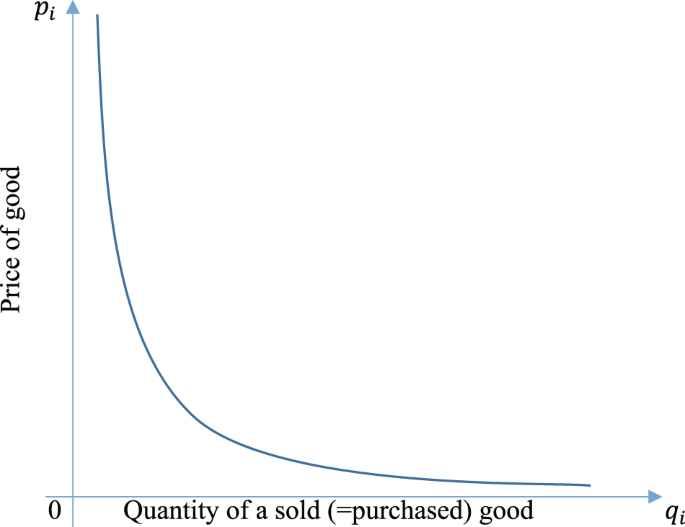

  

  The ‘curve of transactions’ corresponding to the geometric mean index

• c. The index of the purchasing power of money is a weighted (by turnover) geometric average.

  Indeed,

  $$J = \frac{{\bar \omega \left( {p^\prime } \right)}}{{\bar \omega \left( {p^{\prime\prime} } \right)}} = \frac{{p_1^{\prime - \alpha _1}p_2^{\prime - \alpha _2} \ldots p_n^{\prime - \alpha _n}}}{{p_1^{\prime\prime - \alpha _1}p_2^{\prime\prime - \alpha _2} \ldots p_n^{\prime\prime - \alpha _n}}}$$

  (21)

  And because from (19) it follows that

  $$\alpha _i = \mathop {\sum}\limits_i {\alpha _i\frac{{\bar p_i\bar q_i}}{{\bar E}}}$$

  then transforming (21), we get:

  $$J = \left[ {\root \bar{E} \of {\left( {\frac{{p_1^{\prime\prime} }}{{p_1^\prime }}} \right)^{\bar p_1\bar q_1} \times \left( {\frac{{p_2^{\prime\prime} }}{{p_2^\prime }}} \right)^{\bar p_2\bar q_2} \times \cdots \times \left( {\frac{{p_n^{\prime\prime} }}{{p_n^\prime }}} \right)^{\bar p_n\bar q_n}} } \right]^{\mathop {\sum}\nolimits_i {\alpha _i} }$$

  The value of the constant coefficient ∑_iα_i is determined based on the assumption, made when computing any of the indexes of the purchasing power of money: if all the prices increased or decreased by the same number then this means that the purchasing power of money decreases or increases by the same number. Mathematically, this means that the purchasing power of money $\bar \omega \left( {p_1,p_2, \ldots ,p_n} \right)$ is a homogeneous function of degree −1 with respect to p₁, p₂, … , p_n and, consequently, it follows that:³⁸

  $$p_1\frac{{\partial \bar \omega }}{{\partial p_1}} + p_2\frac{{\partial \bar \omega }}{{\partial p_2}} + \cdots + p_n\frac{{\partial \bar \omega }}{{\partial p_n}} = - \bar \omega$$

  or

  $$p_1\frac{{\partial \log \bar \omega }}{{\partial p_1}} + p_2\frac{{\partial \log \bar \omega }}{{\partial p_2}} + \cdots + p_n\frac{{\partial \log \bar \omega }}{{\partial p_n}} = - 1$$

  Using expression (17) for the logarithmic derivatives of $\bar \omega$, we find that

  $$\mathop {\sum}\limits_i {\alpha _i = 1}$$

  (22)

  Therefore, we obtained a formula of the index of the purchasing power of money as a geometric mean of relative changes of prices of goods, weighted proportionally to the turnover of the given goods:³⁹

  $$J = \left[ {\root {{\mathop {\sum}\nolimits_i {\bar p_i\bar q_i} }} \of {{\left( {\frac{{p_1^{\prime\prime} }}{{p_1^\prime }}} \right)^{\bar p_1\bar q_1} \times \left( {\frac{{p_2^{\prime\prime} }}{{p_2^\prime }}} \right)^{\bar p_2\bar q_2} \times \, \cdots \, \times \left( {\frac{{p_n^{\prime\prime} }}{{p_n^\prime }}} \right)^{\bar p_n\bar q_n}}}} \right]$$

  (23)

  Regardless of which period’s turnover would be taken for the weights of the index: base, current or any other intermediate period, because, as was proven above, the share of the turnover of each product in the overall turnover of the country is constant.

  Based on Section 5, it is easy, conversely, to make the following conclusion: an index calculated using a geometric mean, weighted by the turnover share, assumes that the quantities of transacted goods change counter-proportionally to the prices and proportionally to the quantity of money paid for all the goods.

• d. It is not difficult to derive an equation determining the purchasing power of money as a function of the quantities of goods and money, exchanged for each other:

$$\omega = C\left( {\frac{{q_1}}{{\bar p_1\bar q_1}}} \right)^{\frac{{\bar p_1\bar q_1}}{{\bar E}}} \times\, \left( {\frac{{q_2}}{{\bar p_2\bar q_2}}} \right)^{\frac{{\bar p_2\bar q_2}}{{\bar E}}} \times \cdots \times \left( {\frac{{q_n}}{{\bar p_n\bar q_n}}} \right)^{\frac{{\bar p_n\bar q_n}}{{\bar E}}} \times \frac{{\bar E}}{E}$$

(24)

This equation establishes that an index of the ‘volume of trade’ is equal to a weighted geometric mean of the relative changes of quantities of transacted goods, weighted according to the turnover.

Considering the just obtained conclusions, we cannot pinpoint any contradictions to reality in them. We note, first of all, that from Eq. (16), which defines the formula for the function of the purchasing power of money in this section, it follows that if the price of any good turns into zero, then the purchasing power of money goes to infinity; if, conversely, the price of any good goes to infinity, then the purchasing power of money goes to zero. This consequence is consistent with the initial assumption that the `utility of goods and techniques of their production do not change’, since the latter excludes the possibility of the price turning to zero or going to infinity.⁴⁰

The most interesting result is the provision that the weighted by turnover geometric mean form of the index entirely follows on from an almost obvious (especially from the perspective of the index number methodology) assumption: a relative change of the purchasing power of money is determined by the relative changes in prices. The law of the turnover of goods, which is assumed with the geometric mean index: ‘the share of the turnover of each good in the overall turnover of a country is constant’ can find some support in statistical-economic studies, if not with respect to some goods, then, at least with respect to key groups of goods.⁴¹ Therefore, the geometric mean gives correct results for determining the changes of the purchasing power of money only in such cases when there are no strong perturbations in utilities from goods, in the techniques of their production and in the structure of the entire economy. Given the latter, it is worth pointing out that during periods of high inflation, the geometric mean index (as with any other index) will indicate the changes of the purchasing power of money incorrectly.

We also note that we think it is incorrect to follow a commonly practiced method of calculating the geometric mean indexes from month to month with fixed weights. The shares of the turnover of some goods are substantially changing across seasons and therefore it is only possible to calculate the index once per year: by comparing the month of the current year to the corresponding month of the previous year, and by weighting the index for each month according to the turnover shares of the same month in the base period. The ratio of the two indexes calculated this way for two months of the same year will give us an index with the base in the first month, which will be free from seasonal effect. This is justified, of course, only in such a case, if during all the months of the base years, the purchasing power of money remains constant.⁴²

6.3 9. The ‘ideal’ index formula of I. Fisher

Professor Irving Fisher in his work dedicated to price indexes “The Making of Index Numbers”⁴³, based on a series of considerations, proposed the following formula for the purchasing power of money as the best one:

$$J = \sqrt {\frac{{\left( {q_1^{\prime\prime} p_1^{\prime\prime} + q_2^{\prime\prime} p_2^{\prime\prime} + \cdots + q_n^{\prime\prime} p_n^{\prime\prime} } \right)\left( {q_1^\prime p_1^{\prime\prime} + q_2^\prime p_2^{\prime\prime} + \cdots + q_n^\prime p_n^{\prime\prime} } \right)}}{{\left( {q_1^{\prime\prime} p_1^\prime + q_2^{\prime\prime} p_2^\prime + \cdots + q_n^{\prime\prime} p_n^\prime } \right)\left( {q_1^\prime p_1^\prime + q_2^\prime p_2^\prime + \cdots + q_n^\prime p_n^\prime } \right)}}}$$

(25)

where $q_1^\prime ,q_2^\prime , \ldots ,q_n^\prime$ - quantities of goods transacted in the first period, $p_1^\prime ,p_2^\prime , \ldots ,p_n^\prime$ - prices of goods in the first period, $q_1^{\prime\prime} ,q_2^{\prime\prime} , \ldots ,q_n^{\prime\prime}$ - quantities of goods transacted in the second period, $p_1^{\prime\prime} ,p_2^{\prime\prime} , \ldots ,p_n^{\prime\prime}$ - prices of goods in the second period.

This formula, called by Fisher as ‘ideal’ is a geometric mean of two aggregative indexes, where one is weighted by the quantities of goods transacted in the base period and the other by the quantities of goods transacted in the current period.⁴⁴

As we can see, coefficients q in the `ideal’ formula are variable quantities, because they are changing both with the change in the base period and with the change of the current period. Therefore, for the determination of the functional form of the purchasing power of money, we cannot directly use the method that was outlined above in the case of the aggregative index. Let us first make a few transformations of the formula (25), and then work out which functional form of the purchasing power of money corresponds to it and which form of dependency should exist between prices and quantities of transacted goods.

When the purchasing power of money does not change, its index equals 1. Thus this condition implies the following equation:

$$1 = \sqrt {\frac{{{\sum} {p^{\prime\prime} q^{\prime\prime} } }}{{{\sum} {p^\prime q^{\prime\prime} } }} \times \frac{{{\sum} {p^{\prime\prime} q^{\prime} } }}{{{\sum} {p^\prime q^\prime } }}}$$

or

$$\frac{{{\sum} {p^{\prime\prime} q^{\prime\prime} } }}{{{\sum} {p^\prime q^\prime } }} = \frac{{{\sum} {p^\prime q^{\prime\prime} } }}{{{\sum} {p^{\prime\prime} q^\prime } }}$$

(26)

It is assumed as a condition that the purchasing power of money that exists in one period of time is equal to the purchasing power of money that exists in another period of time.

Equation (26) was already considered by us in the context of the theory of indexes for the cost of living. It was a condition of approximate equality of the living standards in two different periods of time.⁴⁵ It can be shown that in this context, if Eq. (26) holds, then the purchasing power of money in the two periods of time is approximately the same. Or, more precisely: if the turnover of one period of time is related to the turnover in another period of time in the same way as the monetary value of the goods of the first period, calculated according to prices of the second period, is related to the monetary value of the goods of the second period, calculated according to prices of the first period, then the possible deviations of the purchasing power of money in one period of time from the purchasing power in the other period are bounded in between some limits.

Assuming that the “ideal formula” of the index of Irving Fisher shows the relative changes in the purchasing power of money not just approximately but exactly, we can consider Eq. (26) as the differential equation of the manifold of equilibrium of the purchasing power of money (hypersurface $\bar \omega \left( {p_1,p_2, \ldots ,p_n} \right) = const$).

This equation, in combination with the obvious assumption that we already made above—if all prices simultaneously increase or decrease by the same proportion then this means that the purchasing power of money decreases or increases by the same proportion—allows us to find the following functional form for the purchasing power of money:

$$\bar \omega \left( {p_1,p_2, \ldots ,p_n} \right) = \frac{1}{{\sqrt {\mathop {\sum}\nolimits_k {\mathop {\sum}\nolimits_i {C_{ik}p_ip_k} } } }}$$

(27)

where C_ik are constant coefficients such that i and k are indicating the particular goods.⁴⁶

In conclusion, the representation for $\bar \omega \left( {p_1,p_2, \ldots ,p_n} \right)$ given by (27), follows from the following arguments.

Based on Eq. (14), and applying the assumptions and notation laid out above [in section 8], the condition (26) can be written in the following form⁴⁷

$$\frac{{\mathop {\sum }\nolimits_i \dfrac{{\partial \bar \omega \left( {p^{\prime\prime} } \right)}}{{\partial p_i^{\prime\prime} }}p_i^{\prime\prime} }}{{\mathop {\sum }\nolimits_i \dfrac{{\partial \bar \omega \left( {p^\prime } \right)}}{{\partial p_i^\prime }}p_i^\prime }} = \frac{{\mathop {\sum }\nolimits_i \dfrac{{\partial \bar \omega \left( {p^{\prime\prime} } \right)}}{{\partial p_i^{\prime\prime} }}p_i^\prime }}{{\mathop {\sum }\nolimits_i \dfrac{{\partial \bar \omega \left( {p^\prime } \right)}}{{\partial p_i^\prime }}p_i^{\prime\prime} }}$$

(26a)

which is a differential equation with partial derivatives and mixed variables.⁴⁸ For the sake of a more concise notation, make the following definitions:

$$\begin{array}{*{20}{c}} \displaystyle{\mathop {\sum}\limits_i {\frac{{\partial \bar \omega \left( {p^{\prime\prime} } \right)}}{{\partial p_i^{\prime\prime} }}p_i^{\prime\prime} = P^{\prime\prime} ;} } & \displaystyle{\mathop {\sum}\limits_i {\frac{{\partial \bar \omega \left( {p^\prime } \right)}}{{\partial p_i^\prime }}p_i^\prime = P^\prime}} \end{array}$$

(a)

Using this notation, Eq. (26a) can be written as follows:

$$\mathop {\sum}\limits_i {P^{\prime\prime} \times p_i^{\prime\prime} \times \frac{{\partial \bar \omega \left( {p^\prime } \right)}}{{\partial p_i^\prime }}} = \mathop {\sum}\limits_i {P^\prime \times p_i^\prime \times \frac{{\partial \bar \omega \left( {p^{\prime\prime} } \right)}}{{\partial p_i^{\prime\prime}}}}$$

(b)

In this last relation, which must hold as an identity, for all values of $p_1^\prime ,p_2^\prime , \ldots ,p_n^\prime$ and $p_1^{\prime\prime} ,p_2^{\prime\prime} , \ldots ,p_n^{\prime\prime}$, we can assign any values to the variables of one of these groups and then every time we will obtain, for the function of the other group of variables, the relations with constant coefficients.

It is known that if in the equation of the type (b) with mixed variables for the function of one of the group of variables one assumes the existence of m of linear relations with constant coefficients, then for the function of the other group of variables, there necessarily will exist 2n − m of linear relations with constant coefficients.⁴⁹ In our case, both series

$$P^\prime p_1^\prime ,P^\prime p_2^\prime , \ldots ,P^\prime p_n^\prime ,\frac{{\partial \bar \omega \left( {p^\prime } \right)}}{{\partial p_1^\prime }}, \ldots ,\frac{{\partial \bar \omega \left( {p^\prime } \right)}}{{\partial p_n^\prime }},$$

(c)

$$P^{\prime\prime} p_1^{\prime\prime} ,P^{\prime\prime} p_2^{\prime\prime} , \ldots ,P^{\prime\prime} p_n^{\prime\prime} ,\frac{{\partial \bar \omega \left( {p^{\prime\prime} } \right)}}{{\partial p_1^{\prime\prime} }}, \ldots ,\frac{{\partial \bar \omega \left( {p^{\prime\prime} } \right)}}{{\partial p_n^{\prime\prime}}},$$

(c')

represent, in essence, the same functions, just different in their notation of variables, and so for the functions of one or the other series, we can allow an equal number of linear relations, i.e., m = 2n – m or m = n. Thus, the functions of the series (c) can be connected by only n linear relations with constant coefficients; these relations can be assumed as solved with respect to the last n functions of the series (c), in the form of:⁵⁰

$$\frac{{\partial \bar \omega \left( {p^\prime } \right)}}{{\partial p_k^\prime }} = \mathop {\sum}\limits_i {A_{ki}P^\prime p_i^\prime}$$

(d)

where A_ki are constant coefficients. Inserting these values $\frac{{\partial \bar \omega \left( {p^\prime } \right)}}{{\partial p_k^\prime }}$ into relation (b) and requiring that (b) holds as an identity with respect to $P^\prime p_1^\prime ,P^\prime p_2^\prime , \ldots ,P^\prime p_n^\prime$, we obtain:

$$\frac{{\partial \bar \omega \left( {p^{\prime\prime} } \right)}}{{\partial p_k^{\prime\prime} }} = \mathop {\sum}\limits_i {A_{ik}P^{\prime\prime} p_i^{\prime\prime}}$$

(d')

Because relations (d) and (d^′), related to the corresponding same functions, must be equivalent, then it is necessary that

$$A_{ik} = A_{ki}$$

(e)

Let us now insert the values of derivatives $\frac{{\partial \bar \omega \left( {p^\prime } \right)}}{{\partial p_k^\prime }}$ into the second of formula displayed in (a). Then dropping the upper indexes in the variables $p_1^\prime ,p_2^\prime , \ldots ,p_n^\prime$, we get:

$$\mathop {\sum}\limits_{ik} {A_{ik}p_kp_i = 1}$$

(28)

The obtained relation is not an identity, and thus it will be a necessary condition of feasibility of (b). The object of interest for us is the manifold $\bar \omega = Const$, consisting of one parameter, and so we must assume that in Eq. (28) the coefficients A are the functions of one parameter and then Eq. (26a) is satisfied by the following solution:

$$\bar \omega = F\left( t \right)$$

(29)

where F(t) is any function and t is determined from Eq. (28), where the coefficients A_ik are arbitrary functions of parameter t and satisfy, conditionally, the symmetry conditions (e).

The obtained solution characterizes the manifold of equilibrium of the purchasing power of money, because when $\bar \omega = const.$ Then t = const and the equation will have constant coefficients; and in such a case it will characterize the manifold of the second degree (a conicoid) with a center at the origin of the coordinate system. However, this solution contains a series of arbitrary functions and thus condition (26) alone is not sufficient for the final determination of the functional form of the purchasing power of money, $\bar \omega$.

We now introduce the above-mentioned assumption, which is typically stated when computing any price index, namely that $\bar \omega \left( {p_1,p_2, \ldots ,p_n} \right)$ is a homogeneous function of degree −1, with respect to all its variables p₁, p₂, … , p_n. This assumption will fully determine the form of the function $\bar \omega$.

Indeed, the homogeneity condition will be:

$$\mathop {\sum}\limits_m {p_m^\prime \times \frac{{\partial \bar \omega \left( p \right)}}{{\partial p_m}} = - \bar \omega }$$

(30)

Let us differentiate Eqs. (29) and (28) with respect to any variable p_i, then:

$$\frac{{\partial \bar \omega \left( p \right)}}{{\partial p_i}} = F^\prime \left( t \right)\frac{{\partial t}}{{\partial p_i}}$$

$$2\mathop {\sum}\limits_k {A_{ik}p_k + \left( {\mathop {\sum }\limits_{i,k} A_{ik}^\prime p_ip_k} \right)\frac{{\partial t}}{{\partial p_i}} = 0}$$

where $A_{ik}^\prime$ denotes the derivative of $A_{ik}^\prime$ with respect to t. From the above equations, we find the derivatives $\frac{{\partial \bar \omega \left( p \right)}}{{\partial p_i}}$:

$$\frac{{\partial \bar \omega \left( p \right)}}{{\partial p_i}} = - 2F^\prime \left( t \right)\frac{{\mathop {\sum}\nolimits_k {A_{ik}p_k} }}{{\mathop {\sum}\nolimits_{i,k} {A_{ik}^\prime p_ip_k} }}$$

And we can insert them into (30), and therefore obtain the following equation:

$$\mathop {\sum}\limits_{ik} {A_{ik}^\prime p_kp_i = \frac{{2F^\prime \left( t \right)}}{{F\left( t \right)}}}$$

This last relation must be equivalent to relation (28) and therefore their corresponding coefficients must be proportional. Therefore, for all values i and k (running from 1 to n):

$$\frac{{A_{ik}^\prime }}{{A_{ik}}} = \frac{{2F^\prime \left( t \right)}}{{F\left( t \right)}}$$

Integrating these equations, gives us

$$A_{ik} = C_{ik}\left[ {F\left( t \right)} \right]^2$$

where C_ik are constant coefficients satisfying the condition of symmetry:

$$C_{ik} = C_{ki}$$

If the derived expressions (31) for coefficients A_ik are inserted to Eq. (28), then we obtain the following function for the purchasing power of money:

$$\bar \omega = F\left( t \right) = \frac{1}{{\sqrt {\mathop {\sum }\nolimits_{k,i} C_{ik}p_ip_k} }}$$

(27a)

The hypersurface of the prices that generate the same level for the purchasing power of money is a hypersurface of the second degree with the center at the origin of the coordinate system. In the case of two variables (p₁ and p₂), the curve of the equilibrium of the purchasing power of money, depicted in Fig. 3, is a hyperbola with its center at the origin of the coordinate system. In this case, the function of the purchasing power of money will be

$$\bar \omega \left( {p_1,p_2} \right) = \frac{1}{{\sqrt {C_{11}p_1^2 + 2C_{12}p_1p_2 + C_{22}p_2^2} }}$$

and, therefore, the equation of the curve of the equilibrium will be

$$C_{11}p_1^2 + 2C_{12}p_1p_2 + C_{22}p_2^2 = const.$$

Fig. 3

Curves of equilibrium purchasing power of money corresponding to the index of Irving Fisher

Based on Eqs. (27) and (14), we will obtain the following expression for the purchasing power of money:

$$\omega = \frac{{\sqrt {\mathop {\sum}\nolimits_m {\mathop {\sum}\nolimits_j {C^{mj}q_mq_j} } } }}{E}$$

(32)

where C^mj are constant coefficients while m and j are indicators of particular goods.

The price of a good k, expressed as a function of quantities of transacted goods and the money paid for them, is the following expression:

$$p_k = \frac{{E \mathop {\sum}\nolimits_m {C^{mk}q_m} }}{{\mathop {\sum}\nolimits_m {\mathop {\sum}\nolimits_j {C^{mj}q_mq_j} } }}$$

(33)

where C^mk are constant coefficients, while k, m, j are indicators of particular goods.⁵¹

If we consider that the quantities of all the goods, except for one, do not change, then the price of this good will be the following function of its quantity (the equation of the curve of transaction):

$$p_k = \frac{{E\left( {B_1a_k + B_2} \right)}}{{B_3a_k^2 + B_4a_k + B_5}}$$

where B₁, B₂, … , B₅ are constant coefficients.

The quantity of goods as a function of prices of goods and the quantity of money paid for all these goods, is determined by the following equation, analogous to (33):

$$q_m = \frac{{E\mathop {\sum}\nolimits_i {C_{mi}p_i} }}{{\mathop {\sum}\nolimits_i {\mathop {\sum}\nolimits_k {C_{ik}p_ip_k} } }}$$

(34)

The “ideal” formula of the index of the purchasing power of money, proposed by Irving Fisher, contains, as was described above, variable coefficients. Now we can, based on the obtained form of the function of the purchasing power of money (27), obtain the formula of the same index with constant coefficients.

$$J = \frac{{\bar \omega \left( {p_1^\prime ,p_2^\prime , \ldots ,p_n^\prime } \right)}}{{\bar \omega \left( {p_1^{\prime\prime} ,p_2^{\prime\prime} , \ldots ,p_n^{\prime\prime} } \right)}} = \sqrt {\frac{{\mathop {\sum}\nolimits_i {\mathop {\sum}\nolimits_k {C_{ik}p_i^{\prime\prime} p_k^{\prime\prime} } } }}{{\mathop {\sum}\nolimits_i {\mathop {\sum}\nolimits_k {C_{ik}p_i^\prime p_k^\prime } } }}}$$

(35)

The coefficients in this formula cannot be obtained through determining the quantities of transacted goods and prices in one period of time, as it was in the case of aggregative and geometric mean indexes. These coefficients can be found with the help of equations connecting the quantities of goods with prices, based on data for (n+1)/2 of periods of time for the case of n goods.⁵²

Therefore, the “ideal” formula leads to a complex form of the index and a complex form of dependency between prices and quantities of goods. Consequently, the statistical testing of these dependencies appears to be difficult. The difficulty of such testing is magnified by the condition of the constancy of the overall structure of the economy, because without this condition the “ideal” formula incorrectly represents the changes of the purchasing power of money. The failure of the constancy assumption can be proven by the unacceptability of the so-called “chaining method” (or, according to Fisher, the failure of the “circularity test”), as confirmed by Irving Fisher himself.⁵³

The advantages of the “ideal” formula relative to others, Fisher sees in the satisfaction of the two main tests of suitability of indexes (time reversal test and factor reversal test) proposed by him. It is not difficult to see that the considerations outlined in this article, are mathematically consistent with the satisfaction of the tests he proposed. However, it is worth noting that the aggregative index and the geometric mean index also pass these tests if it is only assumed that the transaction of goods proceeds according to the same laws that are assumed by these indexes.

We believe that currently there are only two indexes deserving attention and competing between each other to measure the purchasing power of money—the “ideal” index and the geometric mean index.⁵⁴ Deciding on which of them is more suitable appears to be impossible without an accurate statistical study.

A.A. Konüs and S.S. Byushgens.

The translation of the article finishes here and our further discussions continues in the Appendices below.

APPENDICES

Appendix A: Commentary

Some of the arguments and proofs of Konüs and Byushgens are not easy to follow. This is understandable since they were developing many totally new concepts and the implications of optimizing behavior were not well understood at the time when they wrote their paper.⁵⁵ Thus in what follows, we will provide derivations and alternative proofs for many of their results using the now standard tools of microeconomic theory.

We follow the authors’ Section 1 analysis and assume that the purchasing power of money function, ω(q, E), is defined as follows:

$$\omega \left( {q,E} \right) = f\left( q \right)/E$$

(A1)

where q = (q₁, q₂, … , q_n) is a nonnegative consumption vector, f is the purchaser’s utility function and E > 0 is total expenditure on commodities during the period under consideration. The authors also introduce P as “the magnitude that is inverse to the purchasing power of money”, which they later identify as the price level. Since 1/P is equal to ω(q, E) and E is equal to $p \cdot q \equiv \mathop {\sum}\nolimits_{i = 1}^n {p_iq_i}$, the inner product of the vectors p and q, we see that the Konüs and Byushgens price level function P(p, E) can be defined as:⁵⁶

$$P\left( {q,E} \right)\,{\equiv}\, E/f\left( q \right) = p {\cdot}q/f\left( q \right)$$

(A2)

We now turn to our explanations for several of the results of Konüs and Byushgens.

Justification for Eq. (7) in Section 1:

Suppose that $q^\ast$ is a strictly positive consumption vector which solves the following utility maximization problem:

$$\mathop {{{{{\mathrm{max}}}}}}\limits_q \left\{ {f\left( q \right):p \cdot q = E;q \ge 0_n} \right\}$$

(A3)

Assuming that f(q) is differentiable, increasing and concave, then the following n+1 Lagrangian first order conditions will characterize an interior solution to the constrained utility maximization problem (A3):

$$\nabla f\left( {q^ \ast } \right) = \lambda ^ \ast p;$$

(A4)

$$p \cdot q^ \ast = E$$

(A5)

where $\nabla f\left( {q^ \ast } \right) \equiv \left[{\dfrac{{\partial f\left( {q^ \ast } \right)}}{{\partial q_1}}, \ldots \dfrac{{\partial f\left( {q^ \ast } \right)}}{{\partial q_n}}} \right] \equiv \left[ {f_1\left( {q^ \ast } \right), \ldots ,f_n\left( {q^ \ast } \right)} \right]$ is the vector of first order partial derivatives of $f(q^\ast)$.⁵⁷ Take the inner product of both sides of Eq. (A4) with the quantity vector $q^\ast$ and solve the resulting equation for λ^*. Use Eq. (A5) to replace $p\,{\cdot}\,q^{*}$ by E. Substitute this solution for $\lambda^\ast$ back into Eq. (A4) and we obtain the following system of inverse demand equations:

$$\begin{array}{*{20}{c}} {p_i = \dfrac{{Ef_i\left( {q^ \ast } \right)}}{{\mathop {\sum }\nolimits_{j = 1}^n f_j\left( {q^ \ast } \right)q_j^ \ast }},} & {i = 1, \ldots ,n} \end{array}$$

(A6)

Konüs and Byushgens later assume that the utility function f(q) is linearly homogeneous so that f(kq) = kf(q) for all scalars k > 0; see their Eq. (8). Euler’s Theorem on homogeneous functions implies that $f\left( {q^ \ast } \right) = q^ \ast \cdot \nabla f\left( {q^ \ast } \right) = \mathop {\sum}\nolimits_{j = 1}^n {f_j\left( {q^ \ast } \right)q_j^ \ast }$. Thus, when f(q) is linearly homogeneous, Eq. (A6) becomes the following set of equations:⁵⁸

$$\begin{array}{*{20}{c}} \displaystyle {p_i = \frac{{Ef_i\left( {q^ \ast } \right)}}{{f\left( {q^ \ast } \right)}},} & {i = 1, \ldots ,n} \end{array}$$

(A7)

Having established Eq. (A7), using (A1) (i.e., ω(q, E) = f(q)/E)) and performing the differentiation in Eq. (7) in the main text, we find that

$$p_i\left( {q,E} \right) \equiv -\frac{{\dfrac{{\partial \omega \left( {q,E} \right)}}{{\partial q_i}}}}{{\dfrac{{\partial \omega \left( {q,E} \right)}}{{\partial E}}}} = \frac{{\dfrac{{f_i\left( q \right)}}{E}}}{{\dfrac{{f\left( q \right)}}{{E^2}}}} = \frac{{f_i\left( q \right)E}}{{f\left( q \right)}}$$

(A8)

for i = 1, … , n and $q=q^\ast$, which is the same system of inverse demand functions as Eq. (A7). Thus, we have provided sufficient conditions to justify Eq. (7) in the authors’ text.

Interpretation of Eqs. (9) and (10) in Section 4:

Using footnote 14 in the main text, we know that E = c(p)f(q) = c(p)u where u is the purchaser’s utility level. Using Shephard’s Lemma (1953; 11), the purchaser’s system of Hicksian demand functions⁵⁹ is given by q_i = u[∂c(p)/∂p_i] for i = 1, … , n. The indirect utility function is u = E/c(p). Substituting the indirect utility function into the Hicksian demand functions gives us the purchaser’s system of market demand functions:

$$q_i = \left[ {\partial c\left( p \right)/\partial p_i} \right]E/c\left( p \right)\,{{{\mathrm{for}}}}\,i = 1, \ldots ,n$$

(A9)

Thus, we have q_i/E=[∂c(p)/∂p_i]/c(p) for i = 1, … , n which are Eq. (9) in the main text. Thus, the functions f_i (p₁, … , p_n) on the right-hand sides of Eq. (9) are equal to [∂c(p)/∂p_i]/c(p) for i = 1, … , n.

Equation (10) in the main text defines the reciprocal of the purchaser’s unit cost function; i.e., the purchasing power of money function is defined as follows:

$$\omega \left( {q,E} \right) \equiv \frac{{f\left( q \right)}}{E} = \frac{{f\left( q \right)}}{{c\left( p \right)f\left( q \right)}} = \frac{1}{{c\left( p \right)}} \equiv \bar \omega \left( p \right)$$

(A10)

Fisher (1911) and the authors defined the purchaser price level function, P(q, E), as the reciprocal of the purchasing power of money function, ω(q, E). Thus, under the assumption of utility maximizing behavior when the utility function is linearly homogeneous, we have:

$$P\left( {q,E} \right) \equiv \frac{1}{{\omega \left( {q,E} \right)}} = \frac{E}{{f\left( q \right)}} = \frac{{c\left( p \right)f\left( q \right)}}{{f\left( q \right)}} = c\left( p \right)$$

(A11)

Thus, the price level function P(q, E) is equal to the unit cost function c(p) that is dual to the linearly homogeneous utility function f(q). The unit cost function c(p) is a non-decreasing, nonnegative, concave and linearly homogeneous function and thus has the same mathematical properties as f(q).⁶⁰

Discussion of the Section 6 constrained optimization problem involving $\bar \omega \left( p \right) = 1/c\left( p \right)$

Suppose f(q) is a continuous, non-decreasing, concave, linearly homogeneous utility function that is positive if q is strictly positive. As was indicated in an earlier editors’ note, the unit cost function c(p) that is dual to the utility function f(q) is defined for p ≥ 0_n as:

$$c\left( p \right) \equiv {{{\mathrm{min}}}}_q\left\{ {p \cdot q:f\left( q \right) \ge 1;\,q \ge 0_n} \right\}$$

(A12)

Using duality theory (e.g., see Diewert (1974; 119)), it can be shown that the utility function f(q) can be recovered if the unit cost function is known. In particular, we have the following expression for $f(q^\ast)$ in terms of c(p) where $q^\ast$ ≥ 0_n:

$$\begin{array}{l}f\left( {q^ \ast } \right) = {{{\mathrm{max}}}}_{u > 0}\left\{ {u:uc\left( p \right) \le p \cdot q^ \ast ;\,{{{\mathrm{for}}}}\,{{{\mathrm{every}}}}\,p \ge 0_n} \right\}\\ \quad \quad \,\;\; = {{{\mathrm{max}}}}_{u > 0}\left\{ {u:uc\left( p \right) \le 1;\,{{{\mathrm{for}}}}\,{{{\mathrm{every}}}}\,p \ge 0_n\,{{{\mathrm{such}}}}\,{{{\mathrm{that}}}}\,p \cdot q^ \ast = 1} \right\}\end{array}$$

(since uc(p) and p · $q^\ast$ are both linearly homogeneous in p, we can normalize the prices p so that p ∙ $q^\ast$ = 1)

$$\begin{array}{l} = {{{\mathrm{max}}}}_{u > 0}\left\{ {u:c\left( p \right) \le 1/u;\,{{{\mathrm{for}}}}\,{{{\mathrm{every}}}}\,p \ge 0_n\,{{{\mathrm{such}}}}\,{{{\mathrm{that}}}}\,p \cdot q^ \ast = 1} \right\}\\ = {{{\mathrm{min}}}}_p\left\{ {1/c\left( p \right):p \ge 0_n\,{{{\mathrm{and}}}}\,p \cdot q^ \ast = 1} \right\}\\ = 1/{{{\mathrm{max}}}}_p\left\{ {c\left( p \right):p \ge 0_n\,{{{\mathrm{and}}}}\,p \cdot q^ \ast = 1} \right\}\end{array}$$

(A13)

Thus⁶¹c(p) attains a maximum with respect to p under the constraint p ∙ $q^\ast$ = 1. Since $\bar \omega \left( p \right) = 1/c\left( p \right)$ and c(p) > 0, it can be seen that $\bar \omega \left( p \right)$ attains a minimum with respect to p under the constraint p ∙ $q^\ast$ = 1.

Derivation of the Cobb-Douglas price index in section 8using unit cost functions.

Assumption (15) made by the authors can be replaced by the following equivalent assumption (A14) where we have replaced the purchasing power of money function, $\bar \omega \left( p \right)$, by $c\left( p \right) = 1/\bar \omega \left( p \right)$ where c(p) is the purchaser’s unit cost function:

$$\frac{{c\left( {p^{\prime\prime} } \right)}}{{c\left( {p\prime } \right)}} = J\left( {\frac{{p_1^{\prime\prime} }}{{p_1^\prime }},\frac{{p_2^{\prime\prime} }}{{p_2^\prime }}, \ldots ,\frac{{p_n^{\prime\prime} }}{{p_n^\prime }}} \right)$$

(A14)

Let J_i denote the partial derivative of $J\left( {\frac{{p_1^{\prime\prime} }}{{p_1^\prime }}, \ldots ,\frac{{p_n^{\prime\prime} }}{{p_n^\prime }}} \right)$ with respect to its i^th argument, $\frac{{p_i^{\prime\prime} }}{{p_i^\prime }}$ for i = 1, … , n. We assume that the first order partial derivatives of c(p) and $J\left( {\frac{{p_1^{\prime\prime} }}{{p_1^\prime }}, \ldots ,\frac{{p_n^{\prime\prime} }}{{p_n^\prime }}} \right)$ exist. Partially differentiate both sides of (A14) with respect to $p_i^{\prime\prime}$ and we obtain an expression for J_i. Partially differentiate both sides of (A14) with respect to $p_i^\prime$ and we obtain another expression for J_i. Equate these two expressions for J_i and after some simplification, we obtain the following expressions for each i:

$$\begin{array}{*{20}{c}} {\dfrac{{p_i^{\prime\prime} c_i\left( {p^{\prime\prime} } \right)}}{{c\left( {p^{\prime\prime} } \right)}} = \dfrac{{p_i^\prime c_i\left( {p^\prime } \right)}}{{c\left( {p^\prime } \right)}},} & {i = 1, \ldots ,n} \end{array}$$

(A15)

Equation (A15) hold for all positive price vectors p′ and p′′. Thus, for each i, each side of equation i in Eq. (A15) must be equal to a non-negative constant, say α_i for i = 1, … , n. The resulting equations are equivalent to the following equations which must hold for all strictly positive price vectors p:

$$\begin{array}{*{20}{c}} {\dfrac{{\partial \ln c\left( p \right)}}{{\partial p_i}} = \dfrac{{\alpha _i}}{{p_i}},} & {i = 1, \ldots ,n} \end{array}$$

(A16)

Equation (A16) constitute a simple system of partial differential equations which have the following solution:⁶²

$$\ln c\left( p \right) = C + \alpha _1\ln p_1 + \cdots + \alpha _n\ln p_n$$

(A17)

which in turn implies a re-normalized geometric mean, or the Cobb-Douglas function; i.e.,

$$c\left( p \right) = e^Cp_1^{\alpha _1} \times \ldots \times p_n^{\alpha _n}$$

(A17a)

The linear homogeneity and monotonicity properties of the unit cost function imply that the constant C is positive and the α_i must sum to 1; i.e., we have:

$$\mathop {\sum}\limits_{i = 1}^n {\alpha _i = 1}$$

(A18)

Note that (A17) is equivalent to (16) in the main text. It should be also noted that the above proof due to the authors is quite different from other axiomatic justifications for the Cobb-Douglas price index. These alternative axiomatic justifications rely on the circularity test for bilateral index number formula of the form P(p¹, p², q¹, q²) where the superscripts on the vectors of prices, p, and vectors of quantities, q, denote time periods.⁶³ The circularity test states that the bilateral index number formula satisfies the equation⁶⁴

$$P\left( {p^1,p^2,q^1,q^2} \right) \times P\left( {p^2,p^3,q^2,q^3} \right) = P\left( {p^1,p^3,q^1,q^3} \right)\;{\rm{for}\; {\rm{any}}\; {\rm{time}}\; {\rm{periods}}\; 1,\; 2,\; 3}.$$

Discussion of (27) and (32) in section 9

Konüs and Byushgens in section 9 developed a method to show which functional forms for the utility function and for the dual cost function are consistent with the use of the Fisher ideal index. Diewert (1976; pp. 141–143) used their method of proof to establish some more general results. What is not clear in section 9 is how exactly did the authors establish a connection between their Eqs. (27) and (32) and so we try to clarify it below. Using our notation, (27) is equivalent to defining the purchaser’s unit cost function as follows:

$$c\left( p \right) \equiv \left( {\mathop {\sum}\limits_{k = 1}^n {\mathop {\sum}\limits_{i = 1}^n {C_{ki}p_kp_i} } } \right)^{\frac{1}{2}}$$

(A19)

where the constants C_ki satisfy C_ki = C_ik for all 1 ≤ k, i ≤ n. Thus c(p) is the square root of a quadratic form in product prices. The author’s Eq. (32) is equivalent to the following equation:

$$f\left( q \right) = \left( {\mathop {\sum}\limits_{m = 1}^n {\mathop {\sum}\limits_{j = 1}^n {C^{mj}q_mq_j} } } \right)^{\frac{1}{2}}$$

(A20)

where the constants C^mj satisfy C^mj = C^jm for all 1 ≤ m, j ≤ n. Thus f(q) is the square root of a quadratic form in product quantities. The authors assert that Eq. (27) follows from (32), i.e., in our notation (A20) follows from (A19), but they do not indicate exactly how this follows or how the C^mj in (A20) relate to the C_ki in (A19). Below, we provide a likely explanation for the authors’ results.

Suppose the purchaser’s unit cost function is defined by (A19) so that c(p) = [p ∙ Cp]^1/2 where C ≡ [C_ik] is the symmetric n by n matrix of constant coefficients that appear in definition (A19).⁶⁵ Eq. (A13) above give us a formula for calculating the utility function f(q) that corresponds to the unit cost function defined by (A19). Let $q^\ast$ be a given positive quantity vector. In order to calculate $f(q^\ast)$ from a knowledge of c(p), we need to solve the constrained maximization problem:

$$\begin{array}{l}{{{\mathrm{max}}}}_p\left\{ {c\left( p \right):p \ge 0_n,\,p \cdot q^ \ast = 1} \right\}\\ \qquad =\, {{{\mathrm{max}}}}_p\left\{ {\left[ {p \cdot {{{\boldsymbol{C}}}}p} \right]^{\frac{1}{2}}:p \ge 0_n,\,p \cdot q^ \ast = 1} \right\}\end{array}$$

(A21)

Since $c\left( p \right) \equiv \left[ {p \cdot {{{\boldsymbol{C}}}}p} \right]^{\frac{1}{2}}$ is assumed to be non-negative for non-negative price vectors p, maximizing the positive square root of p · Cp will be equivalent to maximizing p · Cp. The first order necessary conditions for a positive $p^\ast$ and Lagrange multiplier $\lambda^\ast$ to solve ${{{\mathrm{max}}}}_p\left\{ {p \cdot {{{\boldsymbol{C}}}}p: p\ge 0_n\,{{{\mathrm{and}}}}\,p \cdot q^ \ast = 1} \right\}$ are as follows:

$${{{\boldsymbol{C}}}}p^ \ast = \lambda ^ \ast q^ \ast$$

(A22)

$$p^ \ast \cdot q^ \ast = 1$$

(A23)

Assume that the symmetric matrix C has an inverse, C⁻¹. Premultiply both sides of (A22) by C⁻¹ and we obtain the equation:

$$p^ \ast = \lambda ^ \ast {{{\boldsymbol{C}}}}^{ - 1}q^ \ast$$

(A24)

Take the inner product of both sides of (A24) with $q^\ast$ and use (A23) to obtain the following solution for $\lambda^\ast$:

$$\lambda ^ \ast = 1/\left( {q^ \ast \cdot {{{\boldsymbol{C}}}}^{ - 1}q^ \ast } \right)$$

(A25)

Substitute (A25) back into (A24) and we find that the solution to ${{{\mathrm{max}}}}_p\left\{ {p \cdot {{{\boldsymbol{C}}}}p:p \ge 0_n\,{{{\mathrm{and}}}}\,p \cdot q^ \ast = 1} \right\}$ and to $\max _p\{ {\left[ {p \cdot {{{\boldsymbol{C}}}}p} \right]^{1/2}:p \ge 0_n\,{{{\mathrm{and}}}}\,p \cdot q \ast = 1} \}$ is:

$$p^ \ast = {{{\boldsymbol{C}}}}^{ - 1}q^ \ast /\left( {q^ \ast \cdot {{{\boldsymbol{C}}}}^{ - 1}q^ \ast } \right)$$

(A26)

Thus, $p^\ast \cdot Cp^\ast$ is equal to $q^ \ast \cdot {{{\boldsymbol{C}}}}^{ - 1}{{{\boldsymbol{CC}}}}^{ - 1}q^ \ast /\left( {q^ \ast \cdot {{{\boldsymbol{C}}}}^{ - 1}q^ \ast } \right)^2 = 1/\left( {q^ \ast \cdot {{{\boldsymbol{C}}}}^{ - 1}q^ \ast } \right)$. Finally, take the positive square root of $p^\ast \cdot Cp^\ast$ and use the last equality in (A13) to show that:

$$f\left( {q^ \ast } \right) = 1/c\left( {p^ \ast } \right) = 1/\left[ {p^ \ast \cdot {{{\boldsymbol{C}}}}p^ \ast } \right]^{1/2} = \left[ {\left( {q^ \ast \cdot {{{\boldsymbol{C}}}}^{ - 1}q^ \ast } \right)} \right]^{1/2}$$

(A27)

Thus, the matrix coefficients C^mj in definition (A20) are the elements of the inverse matrix C⁻¹ under our assumption that the original C matrix has full rank n.

It is possible to start with a normalized quadratic functional form for the utility function f(q) and show that the corresponding unit cost function also has a normalized quadratic functional form. To see this, define f(q) as follows for q ≥ 0_n:

$$f\left( q \right) \equiv \left[ {q \cdot {{{\boldsymbol{B}}}}q} \right]^{1/2}$$

(A28)

where B ≡ [b_ij] is a symmetric n by n matrix that has full rank n.⁶⁶

For a positive commodity price vector $p^\ast$, the unit cost function that corresponds to the utility function f defined by (A28) is defined as the solution to the following constrained cost minimization problem:

$$c\left( {p^ \ast } \right) \equiv {{{\mathrm{min}}}}_q\left\{ {p^ \ast \cdot q:\left[ {q \cdot {{{\boldsymbol{B}}}}q} \right]^{1/2} = 1;\,q \ge 0_n} \right\}$$

(A29)

The constraint in (A29) can be replaced by the constraint q ∙ Bq = 1. The first order necessary conditions for $q^\ast$ to solve the problem ${{{\mathrm{min}}}}_q\left\{ {p^ \ast \cdot q:q \cdot {{{\boldsymbol{B}}}}q = 1;\,q \ge 0_n} \right\}$ are the following conditions:

$$p^ \ast = \lambda ^ \ast {{{\boldsymbol{B}}}}q^ \ast$$

(A30)

$$q^ \ast \cdot {{{\boldsymbol{B}}}}q^ \ast = 1$$

(A31)

Since B⁻¹ exists, (A30) implies that:

$$q^ \ast = {{{\boldsymbol{B}}}}^{ - 1}p^ \ast /\lambda ^ \ast$$

(A32)

Substitute this expression for $q^\ast$ into (A31) and solve the resulting equation for $\lambda^\ast$. We find that $\lambda^\ast$ = [$p^\ast$ ∙ B⁻¹ $p^\ast$]^1/2 and substituting this into (A32) and we find that $q^\ast$ = [$p^\ast$ ∙ B⁻¹ $p^\ast$]B⁻¹ $p^\ast$. Thus, we have

$$c\left( {p^ \ast } \right) = p^ \ast \cdot q^ \ast = \left[ {p^ \ast \cdot {{{\boldsymbol{B}}}}^{ - 1}p^ \ast } \right]^{1/2}$$

(A33)

Discussion of the results in section 9

It seems that Konüs and Byushgens implicitly assumed that the rank of their C matrix was full. But Diewert (1976; 134–135) noted that it is not necessary to assume that the rank of C (or B if we start with utility function) is full; there are interesting cases of B and C that are of rank 1 and correspond to interesting preferences. Thus, if the C matrix is equal to cc^┬, where c is a column vector of positive coefficients and c^┬ is the transpose of c (a row vector), then the unit cost function becomes the linear function p∙q which corresponds to Leontief (no substitution) preferences. Thus, the Fisher price (or quantity) index is exact for this class of preferences.⁶⁷ And if the B matrix is equal to bb^┬, where b is a column vector of positive coefficients and b^┬ is the transpose of b, then the corresponding utility function is the linear function b ∙ q. The Fisher price (or quantity) index is also exact for this class of preferences.

The above two special cases lead to preferences and unit cost functions which are globally well behaved. However, in cases where the rank of the C and B matrices is greater than 1, the situation is more complicated.⁶⁸ Diewert (1976; p. 116) noted that the B matrix which appears in definition (A28) must have a positive eigenvalue with a corresponding positive eigenvector and the remaining eigenvalues of B must be negative or zero. A similar property must hold for the C matrix which appears in definition (A20). Diewert and Hill (2010) established more precisely exactly what the region of regularity is for the functional forms defined by (A20) and (A28).

Finally, Diewert (2020b) and Diewert and Feenstra (2019, 2022) showed how concavity could be imposed upon the functional forms defined by (A20) and (A28) without destroying the flexibility of these functional forms for utility functions and unit cost functions by adapting the methods developed by Diewert and Wales (1987) (1988) for imposing the correct curvature conditions on a different class of functional forms.

Below, we clarify how the concavity conditions can be imposed on $c\left( p \right) \equiv \left[ {p \cdot{{{\boldsymbol{C}}}}p} \right]^{\frac{1}{2}}$ where C ≡ [C_ik] is a symmetric n by n matrix of unknown coefficients. Konüs and Byushgens (1926) show that the system of purchaser demand functions that is generated by this functional form is given by their Eq. (34). Let q^t be the purchaser’s period t quantity demanded vector, let p^t be the market price vector for products purchased in period t and let E^t be total expenditure on products in period t. Then Eq. (34) in our notation become the following system of ordinary consumer equations:

$$\begin{array}{*{20}{c}} {q^t = \dfrac{{E^t{{{\boldsymbol{C}}}}p^t}}{{p^t \,\cdot \,{{{\boldsymbol{C}}}}p^t}},} & {t = 1, \ldots ,T^ \ast } \end{array}$$

(A34)

where $T^\ast$ is the number of periods for which data on prices and quantities are available.

The correct curvature conditions on C are imposed in a series of nonlinear regressions. For the stage 1 regression, set the matrix C equal to c¹ c^1′ where c¹ is a column vector and ${{{\boldsymbol{c}}}}^{1^{\prime} } \equiv \left[ {c_1^1, \ldots ,c_n^1} \right]$ is the transpose of c¹. For the stage 2 regression, set C equal to ${{{\boldsymbol{c}}}}^1{{{\boldsymbol{c}}}}^{1^{\prime} } - {{{\boldsymbol{c}}}}^2{{{\boldsymbol{c}}}}^{2^{\prime} }$ where again c² is a column vector and ${{{\boldsymbol{c}}}}^{2^{\prime} } \equiv \left[ {c_1^2, \ldots ,c_n^2} \right]$ is the transpose of c². We also add the linear restriction 1_n ∙ c² = 0 on the coefficients in the c² vector where 1_n is an n-dimensional vector of ones.⁶⁹ For the stage 3 regression, set C equal to ${{{\boldsymbol{c}}}}^1{{{\boldsymbol{c}}}}^{1^{\prime} } - {{{\boldsymbol{c}}}}^2{{{\boldsymbol{c}}}}^{2^{\prime} } - {{{\boldsymbol{c}}}}^3{{{\boldsymbol{c}}}}^{3^{\prime} }$ where c³ is a column vector and ${{{\boldsymbol{c}}}}^{3\prime } \equiv \left[ {c_1^3, \ldots ,c_n^3} \right]$ is the transpose of c³. The restrictions on c² are the same as in stage 2. There are two linear restrictions on c³: 1_n ∙ c³ = 0 and ${{{\boldsymbol{c}}}}_1^3 = 0$. For the stage 4 regression, set C equal to ${{{\boldsymbol{c}}}}^1{{{\boldsymbol{c}}}}^{1^{\prime} } - {{{\boldsymbol{c}}}}^2{{{\boldsymbol{c}}}}^{2^{\prime} } - {{{\boldsymbol{c}}}}^3{{{\boldsymbol{c}}}}^{3^{\prime} } - {{{\boldsymbol{c}}}}^4{{{\boldsymbol{c}}}}^{4^{\prime} }$ where c⁴ is a column vector and ${{{\boldsymbol{c}}}}^{4\prime } \equiv \left[ {c_1^4, \ldots ,c_n^4} \right]$ is the transpose of c⁴. The restrictions on c² and c³ are the same as in stage 3. There are three linear restrictions on c⁴: 1_n ∙ c⁴ = 0, ${{{\boldsymbol{c}}}}_1^4 = 0$ and ${{{\boldsymbol{c}}}}_2^4 = 0$. In theory, we can keep on adding columns until C is equal to the rank n matrix ${{{\boldsymbol{c}}}}^1{{{\boldsymbol{c}}}}^{1^{\prime} } - {{{\boldsymbol{c}}}}^2{{{\boldsymbol{c}}}}^{2^{\prime} } - {{{\boldsymbol{c}}}}^3{{{\boldsymbol{c}}}}^{3^{\prime} } - \cdots - {{{\boldsymbol{c}}}}^{n - 1}{{{\boldsymbol{c}}}}^{n - 1^{\prime} }$. In practice, the procedure will stop at some point when the last estimated c^k vector turns out to be 0_n and the log-likelihood of the model stops increasing. Of course, if _n is large, and the number of periods is small, it will not be possible to estimate a rank n substitution matrix C. However, the suggested estimation procedure will lead to a semiflexible functional form.⁷⁰

To conclude, the 1924 paper by Konüs is rightfully regarded as a landmark in the history of index number theory. But, from the discussions above it can be seen that the present paper by Konüs and Byushgens is also a landmark in the history of index number theory. It stimulated the development of exact and superlative index numbers which are widely used by statistical agencies today. And, it also suggested two classes of very useful flexible functional forms for direct and inverse systems of consumer demand functions which will probably be widely used in the future.

Appendix B: Proof that (A16) follows from (A17) in the Derivation of the Cobb-Douglas function of Konüs and Byushgens

This appendix focuses on the proof that for the system of partial differential equations given in (A16), i.e.,

$$\begin{array}{*{20}{c}} {\dfrac{{\partial \ln c\left( p \right)}}{{\partial p_i}} = \dfrac{{\alpha _i}}{{p_i}},} & {i = 1, \ldots ,n} \end{array}$$

(B1)

the unique solution (up to a constant) is given by (A17), i.e.,

$$\ln c\left( p \right) = C + \alpha _1\ln p_1 + \cdots + \alpha _n\ln p_n$$

(B2)

We note that there are different ways to prove this result, including an indirect way that relies on general theorems in multivariate calculus. For the sake of completeness, here we provide a direct and explicit proof, which involves minimal knowledge of calculus and differential equations (along with the principle of mathematical induction). To do so, first suppose c(p) is a once differentiable function of the scalar variable p which is defined for p > 0. From the theory of ordinary differential equations, we know that the set of solutions to the differential equation $d\ln c\left( p \right)/dp = \alpha p^{ - 1}$ for p > 0 (where α is a constant) is ln c(p) = α ln p + β where β is a constant. Now look at the first equation in (B1) and hold p₂, p₃ , … , p_n constant. Applying the above solution to this ordinary differential equation gives us the following expression for ln c(p₁, p₂ , … , p_n):

$$\ln c\left( {p_1,p_2, \ldots ,p_n} \right) = \alpha _1\ln p_1 + \beta _1\left( {p_2,p_3, \ldots ,p_n} \right)$$

(B3)

where β₁(p₂, p₃ , … , p_n) is constant as far as variations in p₁ are concerned but this “constant” will depend on (p₂, p₃, … , p_n) in general.

Now, look at the second equation in (B1) and hold (p₁, p₃, … , p_n) constant. Applying the above solution to this ordinary differential equation gives us the following expression for ln c(p₁, p₂, … , p_n):

$$\displaystyle \ln c\left( {p_1,p_2, \ldots ,p_n} \right) = \displaystyle \alpha _2\ln p_2 + \beta _2\left( {p_1,p_3,p_4, \ldots ,p_n} \right)$$

(B4)

where β₂(p₁, p₃, p₄, … , p_n) is a “constant” which will depend on (p₁, p₃, p₄, … , p_n) in general. Now equate the two expressions for ln c(p₁, p₂, … , p_n) and solve the resulting equation for β₁(p₂, p₃, … , p_n). The following solution is obtained:

$$\begin{array}{*{20}{l}}\beta _1\left( {p_2,p_3, \ldots ,p_n} \right) &=& \alpha _2\ln p_2 - \alpha _1\ln p_1 \\&&+\, \beta _2\left( {p_1,p_3,p_4, \ldots ,p_n} \right)\end{array}$$

(B5)

The left-hand side of Eq. (B5) does not depend on p₁. Hence the right hand side of (B5) must also not depend on p₁. This means that the function β₂(p₁, p₃, p₄, … , p_n) must have the following form:

$$\begin{array}{*{20}{l}} \beta _2\left( {p_1,p_3,p_4, \ldots ,p_n} \right) &=& \alpha _1\ln p_1 \\&& +\,\beta _2^ \ast \left( {p_3,p_4, \ldots ,p_n} \right)\end{array}$$

(B6)

Note that the new function $\beta _2^ \ast \left( {p_3,p_4, \ldots ,p_n} \right)$ does not depend on p₁ or p₂. Now substitute (B6) into (B4) and we obtain the following expression for ln c(p₁, p₂, … , p_n):

$$\begin{array}{*{20}{l}} \ln c\left( {p_1,p_2, \ldots ,p_n} \right) &=& \alpha _1\ln p_1 + \alpha _2\ln p_2 \\&&+\, \beta _2^ \ast \left( {p_3,p_4, \ldots ,p_n} \right)\end{array}$$

(B7)

Now, look at the third equation in (B1) and hold all elements of p constant except p₃. Applying the above solution to this ordinary differential equation gives us the following expression for ln c(p₁, p₂, … , p_n), we get:

$$\begin{array}{*{20}{l}} \ln c\left( {p_1,p_2, \ldots ,p_n} \right) &=& \alpha _3\ln p_3 \\&&+\, \beta _3\left( {p_1,p_2,p_4, \ldots ,p_n} \right)\end{array}$$

(B8)

where β₃(p₁, p₂, p₄, … , p_n) is a “constant” which will depend on (p₁, p₂, p₄, … , p_n) in general.

Now equate the two expressions (B7) and (B8) for ln c(p₁, p₂, … , p_n) and solve the resulting equation for $\beta _2^ \ast \left( {p_3,p_4, \ldots ,p_n} \right)$. The following solution is obtained:

$$\begin{array}{l}\beta _2^ \ast \left( {p_3, \ldots ,p_n} \right) = - \alpha _1\ln p_1 - \alpha _2\ln p_2 + \alpha _3\ln p_3\\ \qquad \qquad \qquad\qquad +\, \beta _3\left( {p_1,p_2,p_4, \ldots ,p_n} \right)\end{array}$$

(B9)

The left-hand side of Eq. (B9) does not depend on p₁ or p₂. Hence the right-hand side of (B9) must also not depend on p₁ or p₂. This means that the function β₃(p₁, p₂, p₄, … , p_n) must have the following form:

$$\begin{array}{*{20}{l}}\beta _2\left( {p_1,p_3,p_4, \ldots ,p_n} \right) &=& \alpha _1\ln p_1 + \alpha _2\ln p_2 \\&&+\, \beta _3^ \ast \left( {p_4,p_5, \ldots ,p_n} \right)\end{array}$$

(B10)

Now substitute (B10) into (B8) and we obtain the following expression for ln c(p₁, p₂, … , p_n):

$$\begin{array}{l}\ln c\left( {p_1,p_2, \ldots ,p_n} \right) = \alpha _1\ln p_1 + \alpha _2\ln p_2\\ \quad\qquad\qquad\qquad\qquad + \alpha _3\ln p_3 + \beta _3^ \ast \left( {p_4,p_5, \ldots ,p_n} \right)\end{array}$$

(B11)

The above process can be continued until we obtain the following expression for ln c(p₁, p₂, … , p_n):

$$\begin{array}{*{20}{l}} \ln c\left( {p_1,p_2, \ldots ,p_n} \right) &=& \alpha _1\ln p_1 + \alpha _2\ln p_2 \\&&+ \cdots +\, \alpha _n\ln p_n + \beta _n^ \ast\end{array}$$

(B12)

where $\beta _n^ \ast$ is a genuine constant, which we can denote generically as C. (B12) is equivalent to (B2), which is what we needed to prove.

References

Afriat SN (1972) The Theory of International Comparisons of Real Income and Prices. In: Daly DJ (ed.) International Comparisons of Prices and Outputs. National Bureau of Economic Research, New York, p 13–69
Afriat SN (1987) ‘Fisher and Byushgens’, Chapter III.3 in Logic of Choice and Economic Theory, Oxford, pp. 211–221. https://doi.org/10.1093/0198284616.003.0015
Balk BM (2008) Price and Quantity Index Numbers. Cambridge University Press, New York
Barnett WA, Fisher D, Serletis A (1992) Consumer theory and the demand for money. J Econ Lit 30(4):2086–2119
Buscheguennce (Byushgens) SS (1925) Sur une classe des hypersurfaces. Matematisheskii Sbornik 32(4):625–631
Cobb C, Douglas PH (1928) A theory of production. Am Econom Rev 18:139–165
Diewert WE (1974) Applications of Duality Theory. In: Intriligator MD, Kendrick DA (ed.) Frontiers of Quantitative Economics, Vol. II. North-Holland, Amsterdam, p 106–171
Diewert WE (1976) Exact and superlative index numbers. J Econom 4:114–145
Diewert WE (1993) The Early History of Price Index Research. In: Diewert WE, Nakamura AO (eds.) Essays in Index Number Theory, Volume 1. North-Holland, Amsterdam, p 33–65
Diewert WE (2018) Scanner Data, Elementary Price Indexes and the Chain Drift Problem, Discussion Paper 18-06. Vancouver School of Economics, University of British Columbia, Vancouver, B.C., Canada, V6T 1L4
Diewert WE (2020a) The Axiomatic or Test Approach to Index Number Theory, Discussion Paper 20-03. Vancouver School of Economics, The University of British Columbia, Vancouver, Canada, V6T 1L4
Diewert WE (2020b) Quality Adjustment Methods, Discussion Paper 20-08. Vancouver School of Economics, The University of British Columbia, Vancouver, Canada, V6T 1L4
Diewert WE, Feenstra R (2019) Estimating the Benefits of New Products: Some Approximations, Discussion Paper 19-02. Vancouver School of Economics, University of British Columbia, Vancouver, B.C., Canada, V6T 1L4
Diewert WE, Feenstra R (2022) Estimating the Benefits and Costs of New and Disappearing Products, in Big Data for Twenty-First-Century Economic Statistics, Katharine G. Abraham, Ron S. Jarmin, Brian C. Moyer and Matthew D. Shapiro (eds.), Chicago: University of Chicago Press. pp 437–473
Diewert WE, Hill RJ (2010) Alternative Approaches to Index Number Theory. In: Diewert WE, Balk BertM, Fixler Dennis, Fox KevinJ, Nakamura AliceO (eds.) Price and Productivity Measurement. Trafford Press, Victoria Canada, p 263–278
Diewert WE, Wales TJ (1987) Flexible functional forms and global curvature conditions. Econometrica 55:43–68
Diewert WE, Wales TJ (1988) A normalized quadratic semiflexible functional form. J Econom 37:327–342
Eichhorn W (1976) Fisher’s tests revisited. Econometrica 44(2):247–256
Eichhorn W (1978) Functional Equations in Economics. Addison-Wesley Publishing Company, Reading, MA
Fisher I (1911) The Purchasing Power of Money. Macmillan, London
Fisher I (1922) The Making of Index Numbers. Houghton-Mifflin, Boston
Frisch R (1936) Annual survey of general economic theory: the problem of index numbers. Econometrica 4:1–39
Hicks JR (1940) The valuation of the social income. Economica 7:105–140
Hicks JR (1942) Consumers’ surplus and index numbers. Rev Econ Stud 9:126–137
Hicks JR (1946) Value and Capital, Second Edition. Clarendon Press, Oxford
Hotelling H (1935) Demand functions with limited budgets. Econometrica 3:66–78
Klein JL (1999) The Rise of ‘Non-October’ Econometrics: Kondratiev and Slutsky at the Moscow Conjuncture Institute. Hist Polit Econ Spring 33(1):137–168
Kondratieff ND (1925) The Conjuncture Institute at Moscow. Q. J Econ 39:320–324
Konüs AA (1924) The Problem of the True Index of the Cost of Living, Economic Bulletin of the Conjuncture Institute, No. 9–10, 64–71
Konüs AA (1939) The Problem of the True Index of the Cost of Living, Econometrica 7, 10–29. Originally published (in Russian) in the Economic Bulletin of the Conjuncture Institute (1924), No. 9–10, 64–71
Konüs AA, Byushgens SS (1926) K probleme pokupatelnoi sily deneg. Voprosy Konyunktury 2(1):151–172. (English translation of Russian title: “On the problem of the purchasing power of money)
Laspeyres E (1871) Die Berechnung einer mittleren Waarenpreissteigerung. Jahrb Nationalökonomie Statistik 16:296–314
Olsson C-A (1971) The Cobb-Douglas or the Wicksell Function? Econ Hist 14(1):64–69
Paasche H (1874) Über die Preisentwicklung der letzten Jahre nach den Hamburger Borsennotirungen. Jahrb Nationalökonomie Statistik 12:168–178
Pollak RA (1971) The Theory of the Cost of Living Index, Research Discussion Paper 11, Bureau of Labor Statistics, Washington, DC. Published in Price Level Measurement, ed. W.E. Diewert and C. Montmarquette. Ottawa: Statistics Canada, 1983, 87–161.
Samuelson PA (1947) Foundations of Economic Analysis. Harvard University Press, Cambridge, MA
Samuelson PA (1953) Prices of factors and goods in general equilibrium. Rev Econ Stud 21:1–20
Samuelson PA, Swamy S (1974) Invariant economic index numbers and canonical duality: survey and synthesis. Am Econ Rev 64:566–593
Schultz H (1939) A misunderstanding in index-number theory: the true Konus condition on cost-of-living index numbers and its limitations. Econometrica 7(1939):10–29
Shephard RW (1953) Cost and Production Functions. Princeton University Press, Princeton
Vogt A, Barta J (1997) The Making of Tests for Index Numbers. Physica-Verlag, Heidelberg
Wold H (1944) A synthesis of pure demand. Anal Skandinavisk Aktuarietidskrift 27:69–120
Acknowledgements
We thank Bert Balk, Hideyuki Mizobuchi, Victor Turchin, Evelyn Smart and others who provided their feedback to various versions of this manuscript. Partial financial support from The University of Queensland and ARC grant (FT170100401) is acknowledged.
Funding
Open Access funding enabled and organized by CAUL and its Member Institutions.
Author information
Authors and Affiliations
Corresponding author
Ethics declarations
Conflict of interest
The authors declare no competing interests.
Additional information
Publisher’s note Springer Nature remains neutral with regard to jurisdictional claims in published maps and institutional affiliations.