Joint travel problem in space–time multi-state supernetworks

Abstract

Joint travel problem (JTP) is an extension of the classic shortest path problem and relevant to shared mobility. A pioneering endeavor via supernetwork framework has been put forward to model two-person JTP. However, it was only addressed in the static context and with the assumption of zero waiting disutility, which resulted in no or weak synchronization among the travelers. This paper proposes a space–time multi-state supernetwork framework to address JTP for conducting one joint activity in the time-dependent context. Space–time synchronization and various choice facets related to joint travel are captured systematically. Two-person JTP is first discussed in a uni-modal transport network, and further extended to incorporate multi-modal and multi-person respectively. Stage-wise recursive formulations are proposed to find the optimal joint paths. It is found that JTP is a variant of Steiner tree problem by reduction and the number of meeting/departing points has no impact on the run-time complexity in space–time multi-state supernetworks.

Introduction

Undertaking joint travel is an important part of individuals’ daily lives. The pursuits of joint travel generally result from the psychological needs for interactions with others or from physical constraints such as vehicle-deficiency or being present at the same destinations for shared activities. In part, joint travel is also stimulated by economic and environmental incentives such as HOV/HOT lanes and carpooling/ridesharing initiatives (Nourinejad and Roorda 2016; Sánchez et al. 2016). As evidenced by travel surveys (e.g., Dubernet and Axhausen 2013; Gupta and Vovsha 2013; Ho and Mulley 2015; Liao et al. 2017), a significant portion of a region’s travel is implemented jointly. With the widespread use of social media and location-based services, joint travel is expected to constitute an increasing share of daily travel patterns.

Joint travel problem (JTP), an extension of the classic shortest path problem (Dijkstra 1959), aims to find the optimal joint path for a travel group. A joint path involves multiple individual paths corresponding to multiple origins and destinations. Some parts of the individual paths may be shared by a subset of the travel group. JTP is at the core of ridesharing systems (Furuhata et al. 2013) and has implications for household and social travel (Auld and Zhang 2013; Kang et al. 2013). JTP in nature involves high choice dimensionalities along the trip chains. When a group of individuals opts to travel together, they have to make decisions on where and when to meet. Similarly, at the end of the joint trips, the individuals also need to decide where and when to depart. If more than two persons are involved, choice of meeting/departing sequencing should also be made. Although numerous studies have been conducted to examine joint travel patterns, meeting/departing points have been primarily limited to activity locations. The representation of intermediate meeting/departing points has recently received attention in two-person scheduling models (Liao et al. 2013a; Aissat and Oulamara 2014; Stiglic et al. 2015; Fu and Lam 2016). However, the choice of meeting/departing time/point/sequencing and space–time synchronizations under trip chains and time-dependency have not been addressed in an integrative and efficient manner.

In view of the advantages of network extensions, a supernetwork-based framework has been proposed to address two-person JTP for conducting one joint activity (Liao et al. 2013a). Following the behavioral assumption of minimizing group disutility, three variants of two-person JTP and the corresponding solution algorithms were presented. To capture the decisions on meeting and departing from each other, networks were then differentiated in terms of states, i.e. travel separately or jointly with which transport mode and which activities being conducted. Despite the merits, the framework only addressed JTP in the static context and with the assumption of zero disutility for waiting. As widely recognized, time-dependency is a common phenomenon and joint travel is subject to coupling constraints restricting that individuals must be corporeally present at the same time and location. If one arrives earlier at a meeting point, s/he has to wait and waiting means different levels of disutility to different individuals. To achieve better coordination among the travelers, it is necessary to incorporate the tradeoff between departure time, waiting and activity-travel time-dependency along the joint travel patterns. The ignorance of these components in JTP tends to result in no or weak space–time synchronization.

The purpose of this paper is therefore to propose an improved multi-state supernetwork framework to address JTP in the time-dependent context. Particularly, it relaxes the assumption of “zero waiting disutility” in Liao et al. (2013a). To accommodate space–time synchronization, the time dimension is discretized and multi-state supernetworks are extended in space–time. The derived property remains that any joint path through the space–time supernetworks expresses a joint travel pattern. JTP is first addressed in a uni-modal transport network for conducting one activity and further extended to incorporate multi-modal and multi-person respectively. Stage-wise recursive formulations are proposed to find the optimal joint paths with pseudo-polynomial run-time complexity, which are also the best–worst-case. Analyses on computation complexity of different JTP variants are also presented. It is found that JTP is a variant of Steiner tree problem and the number of meeting/departing points has no impact on the run-time complexity. The proposed framework has applications in joint travel navigation, ridesharing and activity-based modeling systems. As JTP for conducting multiple activities involves complex context-dependencies, we will address it separately in a forthcoming study.

To that end, the remainder of this paper is organized as follows. In “Preliminaries” section, preliminaries of network-based approaches to travel scheduling are provided on a trip and a joint activity level respectively. Section three discusses the representations and solutions of space–time supernetworks to a set of JTPs. Section four illustrates the proposed approach with numerical examples. Finally, the paper is completed with conclusions and discussions of future work.

Preliminaries

Individual travel scheduling for a trip

Finding the optimal path from an origin to a destination has been intensively studied in computer science and operations research. It has vast applications to transportation-related problems. Given road network $G\left( {N,E} \right)$ with $N$ and $E$ being the sets of nodes and links respectively, a transport mode $c$ and an individual $i$, let $o^{i}$ and $d^{i}$ denote the origin and destination respectively, $\varvec{\beta}_{ic}$ a preference vector on the link attributes such as travel time, monetary cost and comfort etc., and $\varvec{X}_{cl}$ an attribute vector of link $l$ with $c$ ($l \in N$). The disutility on $l$ is defined as $\varvec{\beta}_{ic} \cdot \varvec{X}_{cl}$ (non-negative) in the static context. Thus, based on the principle of minimizing individual disutility, individual travel scheduling is reduced to finding the least disutility path. This problem can be efficiently solved by label setting algorithm with run-time complexity $O\left( {\left| N \right| \cdot { \log }\left| N \right|} \right)$ implemented by binary heap in sparse transport networks ($O\left( {\left| N \right|} \right) = O\left( {\left| E \right|} \right))$, where $\left| N \right|$ and $\left| E \right|$ are the numbers of nodes and links of $G$ respectively.

In case that $G$ is a time-dependent network, the disutility on $l$ is redefined as $\varvec{\beta}_{ic} \cdot \varvec{X}_{cl} \left( t \right)$, where $\varvec{X}_{cl} \left( t \right)$ is the attribute vector given arrival time $t$ at the entry node of $l$. If all link disutilities satisfy FIFO (first-in-first-out) condition, the solution algorithm and run-time complexity stay the same as those in the static context. However, they do not satisfy FIFO in most dynamic transport systems since link disutility is a function of multiple factors (Dean 2004). It means departing later or waiting may lead to less overall disutility. Thus, it is necessary to explore the time dimension to find the optimal path. By discretizing the time frame [$T$] as $t \in \left[ T \right] = \left\{ {0,1,2, \ldots ,T - 1} \right\}$, $G$ is reconstructed as a space–time network with acyclic paths. As a result, a pseudo-polynomial time algorithm exists to find the optimal path based on dynamic programming. Let $n \to w$ be a link of $G$ ($n,w \in N$), $r_{nw} \left( t \right)$ the arrival time at $w$ and $c_{nw}^{i} \left( t \right)$ the disutility of traversing $n \to w$ when departing from $n$ at $t$. If there are parallel links between $n$ and $w$, $r_{nw} \left( t \right)$ and $c_{nw}^{i} \left( t \right)$ represent two vectors after traversing all the parallel links. Let $C_{n}^{i} \left( t \right)$ denote the minimum disutility of arriving at node $n$ and time $t$ by departing from $o^{i}$ at any time. With $C_{n}^{i} \left( t \right)$ initialized as 0 for $n = o^{i}$ and as +$\infty$ for $\forall n \in N/o^{i} ,\forall t \in \left[ T \right]$, a recursive formulation (Eq. 1) adapted from Chabini (1999) finds the optimal schedule. The pseudo-code is given below. In particular, $F_{w}^{i} \left( {r_{nw} \left( t \right)} \right)$ (line 6) is a two-tuple vector recording the preceding link and time instance, which are used for backtracking the optimal path.

$$C_{w}^{i} \left( {r_{nw} \left( t \right)} \right) = \left\{ {\begin{array}{*{20}l} { + \infty ,} \hfill & {{\text{if}}\quad r_{nw} \left( t \right)} \ge T \hfill \\ {\hbox{min} \left( {C_{w}^{i} \left( {r_{nw} \left( t \right)} \right), C_{n}^{i} \left( t \right) + c_{nw}^{i} \left( t \right)} \right),} \hfill & {{\text{if}}\quad r_{nw} \left( t \right)} < T \hfill \\ \end{array} } \right.$$

(1)

With Eq. (1), $C_{n}^{i} \left( t \right), \forall n, \forall t$ is settled down as the least disutility. The optimal departure times and paths are obtained by backtracking from $n$ to $o^{i}$. As indicated by Dean (2004) and Cormen et al. (2009), Eq. (1) leads to the best–worst-case run-time complexity, i.e. $O\left( {T \cdot \left| E \right|} \right)$. It should be noted that the recursive formulation in the space–time network does not depend on travel time FIFO condition as the algorithm brutally processes each link in a time-increasing order.

Joint travel scheduling for one joint activity

Liao et al. (2013a) adopted the concept of multi-state supernetworks (Arentze and Timmermans 2004; Liao et al. 2010) to address two-person JTP for conducting one joint activity. Specifically, an individual multi-state supernetwork is constructed by interconnecting networks assigned to different combinations of activity-vehicle states, where activity state defines which activities have been conducted and vehicle state defines where the private vehicles (if any). Furthermore, to capture joint travel, joint state is introduced to define which traveler(s) is (are) involved. For example, given individual $i$ and $j$, there are two joint states (each consists of one individual) when they travel separately; when they travel together, there is one joint state involving $i$ and $j$; and there are two joint states again after they depart from each other. Two types of links are used to interconnect the joint states.

• (1) Meeting link connecting the same nodes from networks of different joint states with more individuals involved in the end point.

• (2) Departing link connecting the same nodes from networks of different joint states with fewer individuals involved in the end points.

Using a multi-state supernetwork, two-person JTP in a uni-modal transport network is illustrated in Fig. 1 (hexagons and octagons denote individual and shared networks respectively; vertices denote locations). Individual $i$ and $j$ depart from origins $o^{i}$ and $o^{j}$ respectively, and they have two alternative meeting points ($m_{1}$ and $m_{2}$), two alternative activity locations ($a_{1}$ and $a_{2}$), two alternative departing points ($d_{1}$ and $d_{2}$), and destinations $d^{i}$ and $d^{j}$ respectively. Any piece of network is attached with the state information “activity | vehicle | joint”. Let “0” and “1” denote the activity being “not conducted” and “conducted” respectively. As no private vehicle is involved, let “0” denote the vehicle state. Note in the diagram that while meeting links of different meeting points are directed to one shared network, departing links of different departing points are directed to different groups of individual networks. Thus, the networks at the last row also include the information of departing point. The purpose was to backtrack consistent joint paths from the destinations to the origins when the forward search procedure is used. The derived property is that any joint path from $o^{i}$ and $o^{j}$ to $d^{i}$ and $d^{j}$ respectively corresponds to a joint travel pattern. With the assumptions of fixed link disutilities and zero waiting disutility, it takes run-time complexity $O\left( {\left| N \right| \cdot { \log }\left| N \right|} \right)$ to find the optimal joint path by label setting algorithm.

Fig. 1

Supernetwork representation of two-person JTP with uni-modal

JTP in space–time multi-state supernetworks

This section discusses a space–time multi-state supernetwork framework for addressing JTP in time-dependent transport networks based on the choice mechanism of minimizing group disutility. This framework takes into account time-dependency and non-zero waiting disutility. Throughout this paper, the disutility of an individual or a joint path is defined as the sum of the associated link disutilities. If a link is traversed by more than one person, we assume the existence of joint preferences that determine the link disutility. Although there are some other joint decision-making mechanisms, minimizing group disutility is commonly used for group activity-travel scheduling (e.g., Jonsson 2008; Dubernet and Axhausen 2013; Kang et al. 2013). The mechanism implicitly assumes the comparability and transferability of individuals’ utilities. Specifically, JTP aims to find the optimal joint path including choices of departure time, route, meeting/departing time/point/sequencing (if any), and activity location and duration for a travel group who want to conduct one joint activity. We first address two-person JTP with uni-modal, and then incorporate multi-modal and multi-person respectively.

Some basic settings are described as follows. Given $G\left( {N,E} \right)$, link travel times on $E$ have a discrete domain and satisfy FIFO condition. That is to say, given $t$ at node $n$ of a link $n \to w$, the arrival time $r_{nw} \left( t \right)$ at $w$ is the same to any travel subgroup using the same transport mode. Although travel time FIFO condition may be violated in reality, this study retains the assumption, following the majority scheduling literature. Whereas, link travel disutility is personalized and may not meet FIFO condition. Let $I$ and $I '$ be a travel group and a subgroup respectively ($I '\subseteq I)$, $c_{nw}^{I '} \left( t \right)|_{s}$ the disutility of $I '$ traversing $n \to w$ at activity state $s$ by departing from node $n$ and time $t$, and $C_{n}^{I '} \left( t \right)|_{s}$ the minimum disutility of $I '$ arriving at $n$ and $t$ by departing from the respective origins at any time. Meanwhile, disutility of waiting is assumed to be linear with waiting time and $\beta_{n}^{{I'{\text{WT}}}}$ denotes the disutility coefficient of $I'$ for waiting at $n$.

Two-person JTP in a uni-modal transport network

In a uni-modal transport network, there is no transfer between different transport modes. Hence, parking-related choices are not considered when a private vehicle (PV) is used. In a broader sense, public transport (PT) network is also categorized as a uni-modal transport network. In this subsection, the solution to two-person JTP is presented in an accumulative fashion. We first discuss the solution for finding the optimal joint travel pattern for reaching an arbitrary activity location, then proceed to discuss the choice of activity duration, and lastly incorporate the returning travel patterns.

First, we consider a JTP in which individual $i$ and $j$ depart from origins $o^{i}$ and $o^{j}$ respectively for location $a$ to conduct a joint activity. The activity must be conducted during the time window [$u_{a}$,$v_{a}$] of $a$, in which $u_{a}$ and $v_{a}$ are the opening time and closing time respectively. Note that $i$ and $j$ may first meet at a meeting point $m_{p}$ and then travel jointly to $a$, or they travel separately and meet at $a$. If $i$ and $j$ arrive at $a$ earlier than $u_{a}$, they have to wait until $u_{a}$. Supposing there are | $A$ | and $|M$ | elements in the activity location set $A$ and meeting point set $M$ respectively ($a \in A, m_{p} \in M$), this JTP is to find the departure times for both $i$ and $j$, meeting point if any, activity location and the routes that together form the optimal joint path. As only two individuals are involved ($I = ij$), there is no choice of meeting sequencing. This problem resembles the three-point Steiner tree problem in a weighted network, which aims to find a node connecting three existing nodes and making the least total length (Hwang et al. 1992). We refer to this problem as three-point JTP. For better understanding the similarity, the basic Steiner tree problem is formulated is provided as follows. Given a set of required points R and a set of optional points Q, along a link distance function $dist: dist\left( {x,y} \right) \to {\mathbb{R}}^{ + }$ between any two nodes $x, y \in R \cup Q$, the objective is to find a tree $ST = \left( {V_{s} , E_{s} } \right)$ that spans all the required points and possibly uses some of the optional points, i.e. $R \subseteq V_{s} \subseteq R \cup Q$, and such that the total length of the tree $\mathop \sum \nolimits_{{\left( {x,y} \right) \in E_{s} }} dist\left( {x,y} \right)$ is minimized. In static networks, the problem can be solved within polynomial time. In time-dependent networks, three-point JTP with continuous departure-time choice is a NP-hard problem.

Lemma 1

Finding the joint path to the above three-point JTP in the static context is a P problem, while it is NP-hard in the time-dependent context.

Proof

In the static context, link travel disutilities are fixed, invariant of departure times at the links. Three-point JTP can be addressed by interconnecting the elementary least disutility paths from two origins ($o^{i}$ and $o^{j}$) respectively to | $M$ | meeting points plus | $A$ | activity locations, and from | $M$ | meeting points to | $A$ | activity locations. Those least disutility paths are found by running two times one-to-all standard shortest path searches from $o^{i}$ and $o^{j}$ in the respective personalized networks. After aggregating the individuals’ disutilities at the meeting points and activity locations, another standard shortest path search in the shared network is needed to update the minimum disutility at all alternative activity locations. Time synchronization at the locations can be perfectly achieved. By backtracking, the optimal departure times and routes can be found. The overall run-time complexity is $O\left( {\left| N \right| \cdot \log \left| N \right|} \right)$. Thus, the JTP is a P-problem, solvable in polynomial time.

In the time-dependent context, link travel disutilities vary with departure times. First consider non-FIFO networks. By assuming $\beta_{n}^{{i{\text{WT}}}} = \beta_{n}^{{j{\text{WT}}}} = 0$ to $\forall n$ (ignoring waiting) and $c_{nw}^{ij} \left( t \right)|_{s} = + \infty$ to $\forall n \to w$, $\forall t$ (disliking joint travel), the solution to the JTP is simply to find two independent one-to-all minimum disutility paths, each of which is a NP-hard problem (Dean 2004). If the network satisfies FIFO property, by assuming $\left| M \right| = 0$ (no meeting point), $\left| A \right| = 1$ (only one activity location), and $\beta_{n}^{{j{\text{WT}}}} = + \infty$ ($j$ does not like waiting, which restrict that $i$ should always be no later than $j$ arriving at the activity location), the JTP is reduced to a resource constrained shortest path problem, which is also a NP-hard problem (Garey and Johnson 1979; Lozano and Medaglia 2013).

Therefore, the proof is completed. □

To address this JTP in the time-dependent context, we adopt solutions in the discrete time domain. The supernetwork representation of JTP is extended in space–time to accommodate waiting, time-dependency and personalized travel disutilities.

Let $G^{i}$ denote the network of personalized link disutilities of $i$ with the same topology as $G$, and $\bar{G}^{i}$ the space–time network. $\bar{G}^{i}$ is constructed by extending every link of $G^{i}$ at every time instance. Formally, any node of $N$ is firstly expanded into $T$ nodes at every discrete time instance of [$T$]; for $\forall t \in \left[ T \right]$ and $\forall n \to w \in E$, $n$ at $t$ and w at $r_{nw} \left( t \right)$ are connected by a directed link if $r_{nw} \left( t \right) \le T - 1$. Since $i$ is allowed to wait at meeting points, waiting links are added at any $m_{p}$ by linking the time instance from $t$ to $t + 1$, $t \in \left\{ {0,1, \ldots ,T - 2} \right\}$, owing to the linear structure of waiting disutility defined above. Waiting links are also added at any $a$ of $A$ with $t \in \left\{ {0,1, \ldots ,u_{a} - 1} \right\}$ because $i$ has to wait at activity locations before the opening times. In a similar way, $\bar{G}^{j}$ can be constructed for $j$, and $\bar{G}^{ij}$ for $i$ and $j$. In $\bar{G}^{ij}$, $i$ and $j$ always stay together. As $i$ and $j$ may meet at $m_{p}$ or $a$, we use meeting links to interconnect $\bar{G}^{i}$ and $\bar{G}^{j}$ with $\bar{G}^{ij}$ at these nodes. Thus, meeting links originate from $\bar{G}^{i}$ and $\bar{G}^{j}$ to $\bar{G}^{ij}$ at the same time instances and locations. Figure 2 illustrates the space–time multi-state supernetwork, in which only two pairs of meeting links are shown for the sake of clear demonstration. The two bold meeting links denote meeting at location $m_{p}$ and time $t^{\prime}$, while the other two meeting at location $a$ and time $u_{a}$.

Fig. 2

Space–time multi-state supernetwork with uni-modal

As the activity has not been conducted yet in Fig. 2, we set the networks at activity state $s = 0$. With the activity state information, this JTP can be solved by stage-wise forward recursive formulations. Initially, $C_{n}^{i} \left( t \right)|_{0}$ is set as 0 to $n = o^{i}$ and as +$\infty$ to $\forall n \ne o^{i} ,\forall t \in \left[ T \right]$. By extending Eq. (1), $C_{n}^{i} \left( t \right)|_{0}$ is obtained with Eq. (2) in a time-increasing order from $t = 0$ to $t = T - 1$. For convenience of expression, we substitute $r_{nw} \left( {t'} \right)$ with $t$, i.e., $t = r_{nw} \left( {t'} \right)$. Compared with Eqs. (1, 2) accommodates waiting at the meeting points and activity locations. Besides attaching activity state, the pseudo-codes of Eq. (2) require an extension on the “if” condition of those for Eq. (1).

$$C_{w}^{i} \left( t \right)|_{0} = \left\{ {\begin{array}{*{20}l} { + \infty ,} \hfill & {if\,\, t \ge T} \hfill \\ {\hbox{min} \left( {C_{w}^{i} \left( t \right)|_{0} , c_{nw}^{i} \left( {t'} \right)|_{0} + C_{n}^{i} \left( {t^{\prime}} \right)|_{0} } \right),} \hfill & {if\,\, t < T, w \notin M \cup A} \hfill \\ {\hbox{min} \left( {C_{w}^{i} \left( t \right)|_{0} , C_{w}^{i} \left( {t - 1} \right)|_{0} + \beta_{w}^{{i{\text{WT}}}} , c_{nw}^{i} \left( {t^{\prime}} \right)|_{0} + C_{n}^{i} \left( {t^{\prime}} \right)|_{0} } \right),} \hfill & {if \,\, t < T,w \in M \cup A} \hfill \\ \end{array} } \right.$$

(2)

In Eq. (2), waiting disutility is calculated in terms of waiting time and location, irrespective of timing. Other waiting policies, either additive or non-additive, can also be represented by extending Fig. 2 and Eq. (2). As seen from the second condition of Eq. 2, waiting incurs disutility at meeting points or activity locations. In addition, waiting is also allowed at the origins. The initialization of disutilities at the time-expanded origins implicitly indicates the disutility of waiting. The above initialization simply assumes that waiting does not incurs disutility at the origins.

Similar to Eq. (2), we can obtain $C_{n}^{j} \left( t \right)|_{0}$, $\forall t \in T, \forall n \in N$, and therefore the minimum disutility for $i$ and $j$ meeting each other, $C_{n}^{ij} \left( t \right)|_{0}$.

$$C_{n}^{ij} \left( t \right)|_{0} = \left\{ {\begin{array}{ll} {C_{n}^{i} \left( t \right)|_{0} + C_{n}^{j} \left( t \right)|_{0} , n \in A \cup M,} \hfill & {\forall t \in \left[ T \right]} \hfill \\ { + \infty ,} \hfill & {\text{else}} \hfill \\ \end{array} } \right.$$

(3)

After assigning $C_{n}^{ij} \left( t \right)|_{0}$ to $\bar{G}^{ij}$ at $n \in A \cup M$, we continuously use a recursive formulation in a time-increasing order for correcting $C_{n}^{ij} \left( t \right)|_{0}$, $\forall n$, by Eq. (4) with $t = r_{nw} \left( {t'} \right)$. The pseudo-codes for Eq. (4) are no significantly different from those for Eq. (2).

$$C_{w}^{ij} \left( t \right)|_{0} = \left\{ {\begin{array}{*{20}l} { + \infty ,} \hfill & {if\,\, t \ge T} \hfill \\ {\hbox{min} \left( {C_{w}^{ij} \left( t \right)|_{0} ,c_{nw}^{ij} \left( {t'} \right)|_{0} + C_{n}^{ij} \left( {t^{\prime}} \right)|_{0} } \right),} \hfill & { if\,\, t < T, w \notin A} \hfill \\ {\hbox{min} \left( {C_{w}^{ij} \left( t \right)|_{0} , C_{w}^{ij} \left( {t - 1} \right)|_{0} + \beta_{w}^{{ij{\text{WT}}}} , c_{nw}^{ij} \left( {t^{\prime}} \right)|_{0} + C_{n}^{ij} \left( {t^{\prime}} \right)|_{0} } \right),} \hfill & {if\,\, t < T,w \in A} \hfill \\ \end{array} } \right.$$

(4)

$C_{n}^{ij} \left( t \right)|_{0}$, $\forall n, \forall t$, is finally settled as the least disutility. Thus far, the optimal time to start the activity at $a$ is equal to ${\text{argmin}}\left\{ {C_{a}^{ij} \left( t \right)|_{0} } \right\}, t \in \left[ {u_{a} ,v_{a} } \right]$. By backtracking from $a$ to $o^{i}$ and $o^{j}$ respectively, we obtain the optimal joint path. In case that $i$ and $j$ do not like travelling jointly, they would just meet at $a$; to another extremity, if they like traveling jointly very much, they would meet at an early stage; and if $i$ does not like waiting to an extreme level, i.e., $\beta_{n}^{{i{\text{WT}}}}$ being a large value, $j$ needs to wait at one of the meeting points. As the topologies of $\bar{G}^{i}$, $\bar{G}^{j}$ and $\bar{G}^{ij}$ are the same, the total worst-case run-time complexity to this JTP remains $O\left( {\left| E \right| \cdot T} \right)$. As shown, Eqs. (2, 4) are capable of dealing with non-FIFO networks. Even in time-disutility FIFO networks, Eqs. (2, 4) generate better run-time complexity than the label setting algorithm. For example, if $\beta_{n}^{{i{\text{WT}}}}$ and $\beta_{n}^{{j{\text{WT}}}}$ are large, which means the arrival times of $i$ and $j$ at some nodes of $M \cup A$ must be the same, it needs to assess all possible arrival times. For a time instance, the time complexity is $O\left( {\left| N \right| \cdot { \log }\left| N \right|} \right)$; thus, the overall time complexity is $O\left( {T \cdot \left| N \right| \cdot { \log }\left| N \right|} \right)$.

The space–time supernetwork framework allows further extensions. Figure 2 can be extended to include the choice of activity duration and departing time/point. The remainder of the space–time multi-state supernetwork is represented as Fig. 3. Therefore, the complete space–time multi-state supernetwork for two-person JTP in a uni-modal network is the union of Figs. 2 and 3 by overlapping the bottom space–time network of Fig. 2 and the top one of Fig. 3. Let $d_{p}$ be an element of a departing point set $D$ ($d_{p} \in D$) and $\left| D \right|$ the number of elements. In Fig. 3, the bold transaction link denotes $i$ and $j$ conducting the activity at $a$ with duration $t^{\prime} - u_{a}$; the bold travel link from $a$ to $d_{p}$ has time elapse of $v_{a} - t^{\prime}$; and the two bold departing links denote $i$ and $j$ departing from each other at time $v_{a}$ and location $d_{p}$. After conducting the activity via a transaction link, the activity state $s$ is changed from 0 to 1. The change of activity state probably brings changes of link disutilities. This characteristic is well-captured in the representation by attaching activity state information “$|_{s}$”. Unlike Fig. 1, we will disclose that one group of individual networks for all departing points is sufficient to find the optimal joint path.

Fig. 3

Space–time multi-state supernetwork with returning trips

The JTP with returning trips resembles the four-point Steiner tree problem. Two points (one for meeting and another for departing) are used to interconnect four points (two origins and two destinations) that aims to minimize the total length, which we refer to as four-point JTP. A four-point JTP can be seen as two three-point JTPs interconnected by activity transaction links. In the static context, the solution of one four-point JTP can be found by combining the solutions to two independent three-point JTPs. In the time-dependent context, a four-point JTP can be reduced to two three-point JTPs, which means a four-point JTP is at least as hard as a three-point JTP. Therefore, the following corollary is derived.

Corollary 1

Finding the joint path to the above four-point JTP in the static context is a P problem, while it is NP-hard in the time-dependent context.

Before conducting the activity, $C_{n}^{ij} \left( t \right)|_{1}$ is initialized as $+ \infty$, $\forall n, \forall t$. $C_{a}^{ij} \left( t \right)|_{1}$, $t \in \left[ {u_{a} ,v_{a} } \right]$, $\forall a \in A$, are updated by traversing transaction links. Let $t$ be the activity start time at $a$, $t \in \left[ {u_{a} ,v_{a} } \right]$; thus, $i$ and $j$ have at most $v_{a} - t$ discrete choices of activity duration. Let $Z_{a}^{ij} \left( {t, \tau } \right)$ be the disutility of a transaction link at $a$ with start time (time of day) $t$ and duration $\tau$. Hence, we have:

$$C_{a}^{ij} \left( {t + \tau } \right)|_{1} = C_{a}^{ij} \left( t \right)|_{0} + Z_{a}^{ij} \left( {t, \tau } \right), t \in \left[ {u_{a} ,v_{a} } \right],\, t + \tau \in \left[ {u_{a} ,v_{a} } \right],\,a \in A$$

(5)

It should be noted that $Z_{a}^{ij} \left( {t, \tau } \right)$ may take any form and ideally it is a continuous function of activity timing and duration. This feature is little affected if the time resolution is set small in the discrete time domain (e.g., 1 min). Based on Eq. (5) and using a forward recursive formulation in $\bar{G}^{ij}$ at activity state $s = 1$, we readily update $C_{{d_{q} }}^{ij} \left( t \right)|_{1}$, $\forall d_{q} \in D, \forall t$. An direct way to get the least disutility of arriving at $d^{i}$ and $d^{j}$ is to continue applying forward recursive formulations with $C_{{d_{q} }}^{ij} \left( t \right)|_{1}$. However, this process involves assessing $\left| D \right|$ groups of individual networks as shown in Fig. 1 to track the specific departing points. An efficient method is to apply backward formulations from $d^{i}$ at $\bar{G}^{i}$ and $d^{j}$ at $\bar{G}^{j}$ to $\forall d_{q} \in D$ respectively. Let ${\overset{\lower0.5em\hbox{$\smash{\scriptscriptstyle\leftarrow}$}}{C}}{}_{n}^{i} \left( t \right)|_{1}$ be the least disutility for $i$ arriving at $d^{i}$ by departing $n$ at $t$ in $\bar{G}^{i}$ at $s = 1$. ${\overset{\lower0.5em\hbox{$\smash{\scriptscriptstyle\leftarrow}$}}{C}}{}_{n}^{i} \left( t \right)|_{1}$ is formulated as Eq. (6) from a time-decreasing order, $\forall t$, $\forall n \to w \in E$. The pseudo-codes for Eq. (6) require the reversed time loop of those for Eq. (1).

$${\overset{\lower0.5em\hbox{$\smash{\scriptscriptstyle\leftarrow}$}}{C}}{}_{n}^{i} \left( t \right)|_{1} = \left\{ {\begin{array}{*{20}l} { + \infty ,} \hfill & {if \,\,\,t \ge T} \hfill \\ {0,} \hfill & {if\,\,\, t < T, n = d^{i} } \hfill \\ {\hbox{min} \left( {\overset{\lower0.5em\hbox{$\smash{\scriptscriptstyle\leftarrow}$}}{C}{}_{n}^{i} \left( t \right)|_{1} , c_{nw}^{i} \left( t \right)|_{1} + \overset{\lower0.5em\hbox{$\smash{\scriptscriptstyle\leftarrow}$}}{C}{}_{w}^{i} \left( {r_{nw} \left( t \right)} \right)|_{1} } \right),} \hfill & {if\,\,\, t < T,n \ne d^{i} } \hfill \\ \end{array} } \right.$$

(6)

Likewise, we obtain ${\overset{\lower0.5em\hbox{$\smash{\scriptscriptstyle\leftarrow}$}}{C}}{}_{n}^{j} \left( t \right)|_{1}$ to $\forall {\text{t}}, \forall n$. Thus, the least disutility ${\overset{\lower0.5em\hbox{$\smash{\scriptscriptstyle\leftarrow}$}}{C}}{}_{{d_{q} }}^{ij} \left( t \right)|_{1}$ that $i$ and $j$ arrive at $d^{i}$ and $d^{j}$ respectively by leaving $d_{q}$ at time $t$ in $\bar{G}^{ij}$ at $s = 1$ is expressed as,

$${\overset{\lower0.5em\hbox{$\smash{\scriptscriptstyle\leftarrow}$}}{C}}{}_{{d_{q} }}^{ij} \left( t \right)|_{1} = {\overset{\lower0.5em\hbox{$\smash{\scriptscriptstyle\leftarrow}$}}{C}}{}_{{d_{q} }}^{i} \left( t \right)|_{1} + {\overset{\lower0.5em\hbox{$\smash{\scriptscriptstyle\leftarrow}$}}{C}}{}_{{d_{q} }}^{i} \left( t \right)|_{1} ,\,\forall t,\,d_{q} \in D$$

(7)

Consequently, the total least disutility of this JTP with returning trips equals to

$${\text{min }}\left\{ {C_{{d_{q} }}^{ij} \left( t \right)|_{1} + \overset{\lower0.5em\hbox{$\smash{\scriptscriptstyle\leftarrow}$}}{C}_{{d_{q} }}^{ij} \left( t \right)|_{1} } \right\},\,{\text{to}}\,\forall d_{q} , \forall t$$

(8)

The choices of $a$,$\tau$, $d_{q}$ and $t$ that together make the minimum value of Eq. (8) are the optimal activity location, activity duration, departing point and time respectively. All other choice facets are found out by backtracking the joint path to the origins and destinations. In the worst case, it takes $O\left( {\left| A \right| \cdot T^{2} } \right)$ steps to assess all duration choices. By applying bi-directed recursive formulations, it takes run-time complexity $O\left( {\left| E \right| \cdot T} \right)$ to capture where and when $i$ and $j$ meet and depart from each other.

In sum, all relevant choice facets are evaluated in the space–time multi-state supernetwork. The space–time synchronization between $i$ and $j$ are sufficiently captured. The formulations take run-time complexity $O\left( {\left| A \right| \cdot T^{2} + \left| E \right| \cdot T} \right)$ to solve the general two-person JTP, which is pseudo-polynomial. In that sense, two person JTP in time-dependent networks is NP-hard in the weak sense. The correctness of the above formulations is proofed by applying the principle of contradictions (Lemma 2). Without the joint activity, four-point JTP is reduced to the classic two-person carpooling problem (Fig. 4). Similar recursive formulations find the optimal joint path with $O\left( {\left| E \right| \cdot T} \right)$ steps, which is more efficient than label correcting algorithms (Bit-Monnot et al. 2013; Fu and Lam 2016).

Fig. 4

Classic two-person carpooling problem

Lemma 2

The proposed formulations (Eqs. 2–8) find the optimal joint path.

Proof

Inside $\bar{G}^{i}$, $\bar{G}^{j}$ and $\bar{G}^{ij}$, given the initial disutilities at certain time instances and locations, the recursive formulations, Eqs. (2, 4, 6), end up with finding the optimal disutilities at any time instances and locations. It is trivial to prove the correctness of Eqs. (5, 8). Thus, Lemma 2 holds if the disutilities added at the meeting and departing points, Eqs. (3, 7), are correct. Assume that there exists a disutility at node $n$ time $t$ in $\bar{G}^{ij}$ less than $C_{n}^{ij} \left( t \right)|_{0}$ in Eq. (3). Then, either $C_{n}^{i} \left( t \right)|_{0}$ or $C_{n}^{j} \left( t \right)|_{0}$ must be set less, which contradicts Eq. (2). The same logic applies to Eq. (7). Thus, the proposed formulations find the optimal joint path.□

Two-person JTP in a multi-modal transport network

This subsection discusses two-person JTP in a multi-modal transport network, which involves mode changes between PV and PT. Multi-state supernetworks were originated to model multi-modal trip chaining by explicitly representing parking-related choices. Let PVN denote a PV network that can only be accessed by the concerned PV, and PTN the PT network including walking and PT modes. Thus, the transfer link at a parking location from PVN to PTN represents parking, and the opposite represents picking-up. Each parking location creates a vehicle state. Once a PV is parked, all activity-travel episode(s) will take place under this vehicle state, until the vehicle state is changed. As each individual ($i$ or $j$) may be in one of two networks, i.e., PVN or PTN, there are four network combinations where $i$ and $j$ could meet or depart. In this study, we consider two common situations: (1) $i$ drives a PV to pick-up and drop-off $j$ at different locations; and (2) $i$ uses a PV to pick-up $j$ and travel to conduct a joint activity. In both situations, they meet in a shared PVN using $i$’s PV. A shared PVN has the same topology as an individual’s PVN, but their link disutilities may be different. Two other situations can be represented similarly.

The process of the first situation is described as follows. First, $i$ travels in PTN to a parking location for picking-up PV and then travels in PVN to one of the meeting points; at the same time, $j$ travels in PTN to the same meeting point; second, once they meet in the shared PVN, $i$ drives the PV to one of the departing points for dropping-off $j$ (not parking but stopping); third, after departing the shared PVN, they enter into their own networks. According to Sects. 2.2 and 3.1, the process is illustrated in a supernetwork as Fig. 5 with two meeting and two departing points respectively (a pentagon, hexagon and heptagon denote a PVN, PTN and shared PVN respectively; $i$ is underlined in the shared network to denote using i’s PV).

Fig. 5

JTP of picking-up and dropping off

Figure 5 is an extension of Fig. 4 from uni-modal network to multi-modal. Similar to “Two-person JTP in a uni-modal transport network” section, the representation can be turned into a space–time multi-state supernetwork. Thus, stage-wise recursive formulations are capable of finding the optimal joint path. It should be noted that the time dimension in PTN and PVN may be discretized with different resolutions. The movement through different space–time networks should take this fact into account. Let $C_{n}^{i} \left( {t_{\delta } } \right)|_{{s{\text{PT}}}}$ and $C_{n}^{i} \left( {t_{\gamma } } \right)|_{{s{\text{PV}}}}$ be the minimum disutility of activity state $s$ node $n$ at time $t_{\delta }$ and $t_{\gamma }$ in PTN and PVN respectively. Suppose $n$ is a parking location and it takes time $\varGamma_{n}^{{i{\text{PP}}}} \left( t \right)|_{s}$ and disutility ${\rm Z}_{n}^{{i{\text{PP}}}} \left( t \right)|_{s}$ for picking up the PV. Unlike activity duration that may be chosen, the time for picking-up or parking is generally determined by the arrival time. By picking-up (from PTN to PVN), $C_{n}^{i} \left( {t_{\gamma } } \right)|_{{s{\text{PV}}}}$ is updated by Eqs. (9–10):

$$C_{n}^{i} \left( {t_{\gamma } } \right)|_{{s{\text{PV}}}} = \hbox{min} \{ C_{n}^{i} \left( {t_{\gamma } } \right)|_{{s{\text{PV}}}} , C_{n}^{i} \left( {t_{\delta } } \right)|_{{s{\text{PT}}}} + {\rm Z}_{n}^{{i{\text{PP}}}} \left( t \right)|_{s} + \Delta^{{i{\text{PP}}}} \left( {t_{\gamma } ,t_{\delta } } \right)\}$$

(9)

$$\Delta^{{i{\text{PP}}}} \left( {t_{\gamma } } \right) = \beta_{n}^{{i{\text{WT}}}} \cdot \left( {t_{\gamma } - t_{\delta } - \varGamma_{n}^{{i{\text{PP}}}} \left( {t_{\delta } } \right)|_{s} } \right)$$

(10)

where $t_{\gamma }$ is first time instance in PVN that is no less than $t_{\delta } + \varGamma_{n}^{{i{\text{PP}}}} \left( t \right)|_{s}$, and $\Delta^{{i{\text{PP}}}} \left( {t_{\gamma } ,t_{\delta } } \right)$ represents waiting disutility for the time gap via picking-up links. Likewise, considering $n$ as a meeting point, the disutility at $n$ of the shared PVN is updated by Eqs. (11–12):

$$C_{n}^{ij} \left( {t_{\gamma } } \right)|_{{s{\text{PV}}}} = \hbox{min} \{ C_{n}^{ij} \left( {t_{\gamma } } \right)|_{{s{\text{PV}}}} , C_{n}^{i} \left( {t_{\gamma } } \right)|_{{s{\text{PV}}}} + C_{n}^{j} \left( {t_{\delta } } \right)|_{{s{\text{PT}}}} + \Delta^{{i{\text{MT}}}} \left( {t_{\gamma } ,t_{\delta } } \right)\}$$

(11)

$$\Delta^{{i{\text{MT}}}} \left( {t_{\gamma } ,t_{\delta } } \right) = \beta_{n}^{{i{\text{WT}}}} \cdot \left( {t_{\gamma } - t_{\delta } } \right)$$

(12)

where $t_{\gamma }$ is the first time instance in PVN that is no less than $t_{\delta }$, and $\Delta^{{i{\text{MT}}}} \left( {t_{\gamma } ,t_{\delta } } \right)$ represents waiting disutility for the time gap via meeting links. Similarly, we can define the waiting disutility for the time gap via parking and departing links. By applying bi-directed formulations, the worst-case run-time complexity is $O\left( {T \cdot { \hbox{max} }\left\{ {\left| {E_{\text{PTN}} } \right|,\left| {E_{\text{PVN}} } \right|} \right\}} \right)$, where $\left| {E_{\text{PTN}} } \right|$ and $\left| {E_{\text{PVN}} } \right|$ denote the number of physical links in PTN and PVN respectively.

The second situation is a little different from the first in that $i$ has to park the PV before conducting the joint activity. After parking, $i$ and $j$ enter a shared PTN marked by where the car is parked. $i$ and $j$ are bundled together until they depart from each other. This process is illustrated by Fig. 6, which includes two parking locations (p₁ and p₂) and two activity locations (a₁ and a₂). Note that a shared PTN (denoted by an octagon) has the same topology as an individual PTN. For ensuring the consistency of parking and picking-up the PV at the same parking locations, there are as many copies of the shared PTNs at one activity state as the number of parking locations. This manipulation is necessary to trace where the private vehicle is parked. Conversely, using only shared PTN at one activity state will cause inconsistent travel patterns. Again, the network representation can be turned into a space–time multi-state supernetwork (Liao et al. 2010, 2012). The treatments on the movement between the shared PVN and PTN of different time resolutions resemble Eqs. (9–12). The optimal joint path is found with run-time complexity of $O\left( {\left| P \right| \cdot \left| A \right| \cdot T^{2} + T \cdot \hbox{max} \left( {\left| P \right| \cdot \left| {E_{\text{PTN}} } \right|, \left| {E_{\text{PVN}} } \right|} \right)} \right)$, where $\left| P \right|$ is the number of parking locations.

Fig. 6

JTP of picking-up and joint activity participation

A general two-person JTP with multi-modal is completed by adding returning trips. Although $i$ and $j$ may depart from each other in any one of the shared PVN or PTNs, the total run-time complexity remains the same order.

JTP of multi-person

Joint travel by a large group is also of great interest given the popularity of social travel stimulated by social activities. This subsection examines how multi-person JTP ($\left| I \right| > 2$, where $\left| I \right|$ is the number of individuals in $I$) can be addressed in the space–time multi-state supernetwork framework. For simplicity, multi-person JTP is only discussed in a uni-modal transport network. With $\left| I \right| > 2$, another choice facet is the meeting/departing sequencing. For example, considering three individuals $i$, $j$ and $k$, $i$ and $j$ may meet first at one location, then travel jointly to meet $k$ at another location, and lastly travel jointly to an activity location. If the meeting sequencing is free to choose, there are seven (or $2^{\left| I \right|} - 1$) personalized networks interconnected by meeting links before conducting the activity; there are five (or $2 \times \left| I \right| - 1$) if they meet with a fixed sequence successively; and this number decreases to four (or $\left| I \right| + 1$) if they meet only at one location. Figure 7 shows an example of supernetwork representation with mixed meeting sequencing, in which $i$ and $k$ never meet first and thus six personalized networks are interconnected excluding the shared network of $ik$. Hence, the meeting sequencing has strong effects on the number of joint states.

Fig. 7

Illustration of three-person JTP (parallelogram denotes a network)

The representation of multi-person JTP can also be turned to space–time multi-state supernetwork. Stage-wise recursive formulations enable us to find the optimal joint travel patterns detailing the space–time synchronization among all the individuals. A step further is to include returning trips after conducting the joint activity. While Eqs. (2, 4) are adapted for updating disutilities inside the personalized networks, Eqs. (3, 7) are extended for updating the disutilities at meeting/departing points,

$$C_{n}^{{I_{1} I_{2} \ldots I_{R} }} \left( t \right)|_{s} = C_{n}^{{I_{1} }} \left( t \right)|_{s} + C_{n}^{{I_{2} }} \left( t \right)|_{s} + \ldots + C_{n}^{{I_{R} }} \left( t \right)|_{s} ,\quad n \in A \cup M, t \in \left[ T \right],s = 0$$

(13)

$$\overleftarrow {{C_{n}^{{I_{1}^{'} I_{2}^{'} \ldots I_{R'}^{'} }} \left( t \right)|_{s} }} = \overleftarrow {{C_{n}^{{I_{1}^{'} }} \left( t \right)|_{s} }} + \overleftarrow {{C_{n}^{{I_{2}^{'} }} \left( t \right)_{s} }} + \ldots + \overleftarrow {{C_{n}^{{I_{R'}^{'} }} \left( t \right)|_{s} }} ,\quad n \in A \cup D, t \in \left[ T \right],s = 1$$

(14)

where $I_{1} ,I_{2} , \ldots ,I_{R}$ and $I_{1}^{'} ,I_{2}^{'} , \ldots ,I_{R'}^{'}$ are $R$ and $R'$ travel subgroups at the joint states where travelers meet and depart respectively.

The run-time complexity for multi-person JTP is primarily decided by the meeting/departing sequencing. Personal preferences, space–time constraints, and spatial distributions of the origins/destinations have effects on the sequencing. Note that vehicle capacity constraint can also be taken into account for constructing the supernetwork representation. The best–worst-case run-time complexity is $O\left( {\left| I \right| \cdot \left| E \right| \cdot T} \right)$ to traverse $\left| I \right| + 1$ or $2 \cdot \left| I \right| - 1$ personalized networks. The worst worst-case is $O\left( {2^{\left| I \right|} \cdot \left| E \right| \cdot T} \right)$ with complete meeting/departing sequencing possibilities. In this case, JTP resembles the general Steiner tree problem and belongs to NP-hard class in the strong sense, which means no algorithm exist thus far that can find the optimal joint path within polynomial time.

Remarks

The above subsections provide the solutions to JTP in different situations in the time-dependent context based on the choice mechanism of minimizing the group disutility. It turns out that JTP is a variant of Steiner tree problem by reduction. Table 1 shows a summary of JTP variants and the corresponding worst-case run-time complexity using recursive formulations in space–time multi-state supernetworks. Given the topologies of the PVN and PTN, several factors have influences on the computational efficiency. The following algorithmic analyses imply that the proposed space–time supernetwork framework is conceptually feasible for addressing various JTP.

Table 1 Summary of JTP and worst-case run-time complexity

Above all, the resolution of time discretization plays a critical role in the space–time supernetworks. The higher the resolution, the closer the joint path found is to the real optimality. Across different resolutions, the differences may mainly lie in the temporal dimension, as the spatial pattern may be the same when the resolutions are within a particular indifferent range (Liao 2016). Time resolution is a non-issue for traversing links in PTN. Current PT systems in practice use 1 min as the time unit in the timetables. Meanwhile, the speed and distance of walking to access or egress PT stops are generally low and short enough to use 1 min as the resolution. On the contrary, it might be an issue for traversing links in PVNs by car, while it is less obvious for PVNs by slow modes. With the high speed of auto vehicles, the time needed to travel a local road segment is likely to be too small so that $T$ of a time frame should be set large for obtaining high accuracy in the temporal and spatial dimension. Thus, it is challenging to obtain the exact optimal joint paths when applying the approach to large-scale detailed networks. In that regard, JTP gives motivations to develop sound speedup techniques, such as goal-directed search and network contraction, for space–time networks in future studies. Nonetheless, the typical time length of a trip is often limited within 1–2 h even at the regional scale. For incorporating joint travel in travel demand forecasting, accessibility and other mobility-related analyses, a less degree of acceptable accuracy is often allowed. Therefore, $\left| {E_{\text{PVN}} } \right|$ and $T$ could be heavily reduced in hierarchical road networks since local short road segments can be ignored.

Second, the number of alternative parking and activity locations, and activity durations may also contribute to a higher order of run-time complexity than $O\left( {\left| E \right| \cdot T} \right)$. However, the effects fade away in reality by the notion that only a small proportion of alternatives are of interest to the individuals from the demand side. Relevant activity and parking locations can be picked out by location selection models (Liao et al. 2013b). Moreover, activity duration also exudes much coarser resolution than the time discretization in the space–time supernetworks.

Third, the number of individuals theoretically results in an exponential increase in the computation time in the extreme case. However, such a situation also dissolves itself in practice. As indicated in empirical studies, only around 6% of the joint trips are carried out by more than three individuals at the intra-household level (Ho and Mulley 2015). A similar percentage has also been identified at the level of social travel (Dubernet and Axhausen 2013). Even if $\left| I \right|$ is large, space–time constraints and lower–upper bound comparisons often interactively cancel out certain meeting/departing sequencing.

Fourth, the number of meeting/departing points has no effect on the run-time complexity, although it has marginal effects on the computational time due to the summations at those points.

Lastly, although a space–time multi-state supernetwork is conceptually large in scale, it is not necessary to store all the nodes and links before scheduling. As many links are related to one spatial link, they can be processed on-the-fly. The storage is mainly required to save the least disutility and routing information at every time-expanded node. Each copy of space–time network corresponds to space complexity $O\left( {\left| N \right| \cdot T} \right)$. Thus, storage will become an issue only when there are many individuals in the travel group with free meeting sequencing.

Numerical examples

As aforementioned, the stage-wise formulations for JTP have predictable computation performances. The numerical examples mainly serve to exemplify the space–time synchronizations among the individuals at the meeting/departing points. Extensive tests of the solutions in different networks are unnecessary and will not achieve any new conclusions other than those summarized in “Remarks” section. This section presents two numerical examples of JTP, executed with C++ on a PC using one core of Intel^® CPU 2.67 GHz, 8 G RAM. Eindhoven region (The Netherlands) is selected as the study area (Fig. 8).

Fig. 8

Eindhoven region (scale: 1:200,000)

• (1) Roads are classified into three types, i.e. < local priority, regional, highway > (local short road segments are removed). Walking and cycling speeds on these road types are set static as < 5, 6, 0 > and < 15, 18, 0 > in km/h respectively. Car speeds refer to time-dependent profiles (Fig. 9). There are 1740 nodes and 2926 directed links with every link length over 0.15 km. This network scale is reasonable for a class of mobility-related analyses. Node contraction technique (Schultes 2008) can be applied to transform large road networks to the same scale. Suppose travel time is the only factor defining PV link disutilities.

  Fig. 9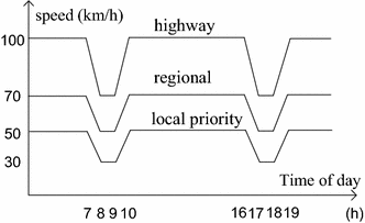

  

  Car speed profiles

• (2) PT timetable is represented in the form of time-dependent network, with 584 stops and 976 links. Bus is the main mode and bus lines follow the hub-and-spoke topology, with three hubs marked in red dots. Bus frequencies vary from 15 min to 1 h. The average bus speed is 36 km/h. There is a bi-directed train connection from Best via Eindhoven (EIN) to Helmond. Waiting and travel time are the two factors for taking PT (ticket cost is compounded with travel time).

• (3) Four persons P1-4 correspond to four home locations H1-4 (in orange). Three workplaces (W1-3), one leisure center (L1), and one restaurant (R1) are in green. Meeting/departing points are selected from PT stops where any two bus lines split as these stops offer transfer opportunities. In total, 30 points (in blue) are selected besides the three hubs.

Two-person JTP

This example emphasizes the choice of where and when to meet. For easiness of interpretation, each individual only uses one transport mode. Suppose a recreational event will take place at L1 with time window [2:00pm, 4:00pm]. Two traveler groups (P1&P2 and P3&P4) plan to participate in the event with transport modes bike and PT respectively. Assume the engagement in the leisure activity produces utility as $u\left( \tau \right) = 20 \cdot \ln \left( {1 + \tau } \right) - 0.25 \cdot \tau$ for the two groups homogeneously, where $\tau$ denotes the duration in minute. This utility function combines the log-shape increase effects of activity duration and the opportunity costs. The disutility coefficients of time for travel and waiting are specified by rule-of-thumb in Table 2 without considering the effects of activity states ($*$ stands for travel group; * = 1 if P1 is involved, and * = 12 if P1&P2 are involved). Note that these parameters should be estimated simultaneously from revealed or stated data, which is beyond the scope of this study.

Table 2 Disutility coefficient of time in 1 min

Figure 10 shows the scheduling results of joint paths from H1 and H2 to L1 by P1&P2 under different settings of $\beta^{{12{\text{B}}}}$. Since P1&P2 use bikes and travel in the static network, space–time synchronization can be perfectly achieved (Lemma 1). The departure times are derived by backtracking the sub-paths in a way that no waiting is involved. As expected, P1&P2 tend to have longer distance jointly traveled when joint travel becomes more and more preferable (decreasing $\beta^{{12{\text{B}}}}$ from 1.6 to 0.6). In Fig. 10a, $\beta^{{12{\text{B}}}}$ is set as the sum of $\beta^{{1{\text{B}}}}$ and $\beta^{{2{\text{B}}}}$, which means joint travel does not reduce disutility; hence, the optimal joint path consists of two separate least-disutility paths, with a total travel distance of 19.2 km. P1&P2 only meet at the last travel stage as they are not geographically distributed in the same direction to L1. As $\beta^{{12{\text{B}}}}$ decreases, P1&P2 meet at earlier stages for attaining more joint travel. When $\beta^{{12{\text{B}}}}$ is equal to 1.1 in Fig. 10b, they meet at EIN somewhere close to the geometric center surrounded by H1, H2, and L1. When $\beta^{{12{\text{B}}}}$ is extremely low, P1&P2 are expected to utilize as much joint travel as possible to reduce the total disutility despite increasing the trip distance. For example, when $\beta^{{12{\text{B}}}} = 0.6$ in Fig. 10c, P1&P2 meet at a point close to H1 with a total travel distance of 22.9 km.

Fig. 10

Joint paths of P1&P2 by bike (M stands for the chosen meeting point). (a) $\beta^{{12{\text{B}}}}$ = 1.6. (b) $\beta^{{12{\text{B}}}}$ = 1.1. (c) $\beta^{{12{\text{B}}}}$ = 0.6

The joint travel paths of the returning trips from L1 to H1 and H2 are exactly the same as the forward trips under the same settings of $\beta^{{12{\text{B}}}}$. The chosen duration for the leisure activity is the one maximizing $u\left( \tau \right)$, which is 79 min.

Figure 11 shows the scheduling results of joint travel patterns for conducting the activity by P3&P4 under different settings of $\beta_{n}^{{*{\text{WTs}}}}$. Due to the topology of the PT system, EIN is both the meeting and departing point. Given the discrete-time nature of PT services, waiting may still occur in the best synchronized situations. In both cases, $\beta_{n}^{{34{\text{WTs}}}} =$ 1.5 and $\beta_{n}^{{34{\text{WTs}}}} =$ 2.5, P3 first waits P4 at EIN and then P3&P4 wait jointly for the bus outbound for L1. The returning trips are similar as they need to wait for bus or train at EIN. When $\beta_{n}^{{34{\text{WTs}}}}$ is lower (1.5), P3&P4 do not mind waiting jointly too much, and they have more freedom for choosing departure time, route and activity duration to attain the least disutility. Although the chosen duration (83 min) is longer than the one deriving the most utility (79 min), it is the outcome of tradeoff for avoiding waiting long for bus to return EIN. However, when $\beta_{n}^{{34{\text{WTs}}}}$ is higher (2.5), P3&P4 avoid waiting long by departing half hour later and taking another bus line. Thereafter, the chosen activity duration is reduced to 60 min. The returning patterns of both cases are exactly the same.

Fig. 11

Joint travel patterns of P3&P4 by PT (EIN is the meeting/departing point)

The above two-person JTP examples show that departure time, meeting/departing time/point and activity duration are interdependent. In the example of using bike, the computation time is trivial. In the example of using PT, the time resolution is 1 min and thus T is reasonably bounded on a trip level. In both examples, the computation times are less than 0.001 s.

Multi-person JTP

This example concerns a four-person JTP with meeting/departing sequencing. Suppose P1-4 have work activity at W1, W1, W2 and W3 respectively and a joint dinner activity at restaurant R1; meanwhile, P1 drives car, and P2-4 take PT to the workplaces in the morning. To highlight the choice of meeting/departing time/point/sequencing for the joint activity, the travel scheduling only focuses on the time period from 5:00 pm when everyone may leave office to the time when everyone arrives at home after dinner. For simplicity, suppose that the dinner lasts at least 2 h with a fixed utility, parking is free at R1, and the car has five seats. Personalized travel preferences are set (Table 3) in a way that all individuals are homogenous and prefer to travel with others. $I^{\prime}$ and | $I^{\prime}$ | denote a travel group ($I^{\prime} \subseteq I$) and the number of persons in $I^{\prime}$ respectively. Although P2-4 do not own cars, they still have preferences of being car passengers. The coefficient setup shows discounting of disutility if more individuals travel jointly.

Table 3 Coefficient of time in terms of disutility by 1 min ($\beta_{1} > \beta_{2} > 0$)

As discussed in “JTP of multi-person” section, there are at most 15 (or $2^{4}$ − 1) personalized networks interconnected by meeting links before starting dinner in the space–time supernetwork. Despite no particular meeting sequencing specified by the individuals, the spatial distribution of the locations automatically remove some meeting sequencing. The following exclusion of joint travel patterns is implemented by prior manual calculations. Consider a joint travel pattern that P1&P2 leave W1 separately (Fig. 12a). Since P1&P2 have to be together again for dinner, suppose they meet again at M2. In-between, P1 and P2 may separately have any interactions with P3 or P4. Then, consider another joint travel pattern that P1&P2 leave W1 jointly (Fig. 12b) with the same interactions with P3 or P4 as the previous one. Based on the setting above, the disutility of the latter pattern is always less than the former. It is because traveling by car is more preferable than by PT and furthermore waiting may occur if P1 and P2 do not arrive at M2 at the same time. In that sense, we infer that P1&P2 should always stay together before reaching R1; and therefore eight personalized networks, i.e., P1, P2, P1&P3, P1&P4, P2&P3, P2&P4, P1&P3&P4 and P2&P3&P4, are not relevant for the optimal joint path.

Fig. 12

Comparison of two joint travel patterns. a P1 and P2 travel separately. b P1 and P2 travel jointly

Similarly, there are at most 15 personalized networks interconnected by departing links for returning trips. We use lower–upper bound comparisons to exclude some personalized networks. Consider a travel pattern that P2&P4 leave R1 together through their shared PTN and depart from each other at a departing point D1 (Fig. 13a). The trip from R1 to D1 involves a combination of walking, waiting and taking PT, which have the upper bound speed of 36 km/h. Then, consider another travel pattern that P1 drops P2&P4 at D1 and drives back to R1 (Fig. 13b), keeping the interaction with P3 as the same as the previous pattern. As the timing after dinner is later than 7:00 pm (off-peak), the lower-bound speed is 50 km/h. With the settings of coefficients, the latter pattern is expected to always produce less disutility than the former. Thus, it implies that P2, P3 and P4 never travel jointly without P1. Thus, P2&P3, P2&P4, P3&P4 and P2&P3&P4 should be excluded.

Fig. 13

Comparison of two joint travel patterns. a Only P2&P4 travel jointly. b P1&P2&P4 travel jointly

With the above reductions, a compact space–time multi-state supernetwork for this JTP is constructed. Stage-wise recursive formulations adapted from Eqs. (2–14) are capable of finding the optimal joint path. Other settings are as follows: $\beta_{1} = 0.6, \beta_{2} = 0.1$, 1 min for boarding/alighting PT, and time resolutions being 10 s and 1 min in PVN and PTN respectively. The scheduling result of the joint travel pattern is shown in Fig. 14, in which EIN is both the meeting and departing point owing to its centric position among the scattered origins/destinations. As shown, space–time synchronizations and all relevant choice facets are well captured. The travel dynamics in PVN and PTN during peak and non-peak times are also incorporated. On the forward trips to R1, as P1&P2 have more freedom of departure time choice with car, they arrive at EIN at the same time as P4 so that only P3 waits 1 min. Whereas, on the returning trips to homes, the dinner is finished at a time allowing P1 to drop-off P2-4 at EIN for PT and cause no waiting time for P2 and short waiting times for P3 and P4.

Fig. 14

Optimal joint travel pattern

The computation time for the four-person JTP is 0.016 s without any speed-up techniques, demonstrating the potential of the suggested approach. The spatial distribution of the locations and the number of meeting/departing locations only have marginal effects on computation time. Although the scales of the PTN and PVN are relatively small compared to those in single point-to-point routing problems, networks of similar coarse resolutions have been adopted for mobility-related analysis at the population level (e.g., Kang et al. 2013; Auld et al. 2016). Thus, the proposed approach is still applicable to activity-based microsimulation systems that allow multiple agents share one episode of joint activity-travel. Regarding its application to joint travel navigation systems, this example also offers insights for reducing the supernetwork scale for multi-person JTP.

Computation time seems a challenge for large-scale applications. Time resolution in PVN does matter. As indicated, the recursive formulations process each link at every discrete time instance at most once, making the optimal computation time complexity in the worst case. To guarantee the accuracy of the scheduling results, the time dimension should be discretized in a high resolution, especially in transport networks with short road segments, which is the major cause of long computation time. In theory, decreasing the time complexity for scheduling in space–time networks remains a challenging topic. However, in practice, there are engineering approaches to speed up the routing procedures. For example, in large transport networks, network partition technique can be applied to select the relevant sub-networks for short distance scheduling queries, and highway hierarchy to overlook irrelevant local roads for long distance queries (Bast et al. 2014).

Conclusions and discussion

A significant share of individuals’ daily travel is implemented jointly and the share is expected to increase with the widespread use of location-based services. JTP tends to have more applications in transportation-related problems. It has also been an important sub-problem of activity-based travel demand analysis (Timmermans and Zhang 2009). This paper proposed a space–time multi-state supernetwork framework to address joint travel scheduling that relaxes an assumption made in a previous study. Two-person JTP with uni-modal was first investigated and extended to multi-modal and multi-person JTP. Recursive formulations were proposed to find the optimal joint travel patterns. Algorithmic analyses and numerical examples were carried out to demonstrate the feasibility of this framework.

Several issues are worth further investigation. First, to achieve accurate synchronizations among the individuals, it is necessary to elicit the personalized preferences and choice making mechanisms on joint activity-travel. Second, the run-time complexities are related to the number of location alternatives for activities and parking. Thus, it is beneficial to develop location selection models that take into account space–time constraints, coupling constraints and vehicle capacity constraints. Third, multiple episodes of joint activities and flexible activity sequence should also be included. In other words, in a larger scope, multi-modal, multi-person and multi-activity should be modeled in a unified framework. This modeling extension relates to a more specific application domain, i.e. activity-based travel demand analysis. However, the supernetwork scale may explode even for two-person JTP given the numerous state combinations. In that sense, various choice rules and heuristics should be developed to construct the space–time supernetworks at reasonable sizes. Fourth, stage-wise recursive formulations are adopted to solve JTPs due to the simplicity and predictable computation performance. As JTP in the time-dependent context is NP-hard, we do not expect a polynomial-time solution algorithm. Label setting algorithm may also be viable in the space–time supernetworks, but it does not obtain a lower order of computation time complexity. There is a research community working on the speedup techniques. While most techniques have been developed in FIFO networks, efficient counterparts should also be developed specifically for non-FIFO (super) networks. Fifth, Travel scheduling under uncertainty has attracted increasing attention in the past years. However, the relevant studies have focused on single travelers. JTP under uncertainty needs the incorporation of space–time coordination at the meeting points. Time of waiting for other people becomes the subtraction of random arrival times. The proposed space–time supernetworks are still a viable framework to incorporate different realizations of uncertain travel times if the temporal dimension is discretized in an even higher resolution. However, this manipulation may involve considerable computation time. These issues will be addressed in future research.

References

Aissat, K., Oulamara, A.: A priori approach of real-time ridesharing problem with intermediate meeting locations. J. Artif. Intell. Soft Comput. Res. 4(4), 287–299 (2014)
Arentze, T.A., Timmermans, H.J.P.: A multi-state supernetwork approach to modelling multi-activity multimodal trip chains. Int. J. Geogr. Inf. Sci. 18, 631–651 (2004)
Auld, J., Zhang, L.: Inter-personal interactions and constraints in travel behavior within households and social networks. Transportation 40(4), 751–754 (2013)
Auld, J., Hope, M., Ley, H., Sokolov, V., Xu, B., Zhang, K.: POLARIS: agent-based modeling framework development and implementation for integrated travel demand and network and operations simulations. Transp. Res. Part C 64, 101–116 (2016)
Bast, H., Delling. D., Goldberg. A., Müller-Hannemann. M., Pajor. T., Sanders. P., Wagner. D., Werneck, R.: Route planning in transportation networks. Technical Report MSR-TR-2014-4, Microsoft Research (2014)
Bit-Monnot, A., Artigues, C., Huguet, M., Killijian, M. Carpooling: the 2-synchronization points shortest paths problem. In: 13th Workshop on Algorithmic Approaches for Transportation Modelling, Optimization, and Systems (ATMOS), Sophia Antipolis, France (2013)
Chabini, I.: Discrete dynamic shortest path problems in transportation applications: complexity and algorithms with optimal runtime. Transp. Res. Rec. 1645, 170–175 (1999)
Cormen, T.H., Leiserson, C.E., Rivest, R.L., Stein, C.: Introduction to Algorithms, 3rd edn. The MIT Press, Cambridge (2009)
Dean, B.: Algorithms for minimum-cost paths in time-dependent networks with waiting policies. Networks 44, 41–46 (2004)
Dijkstra, E.W.: A note on two problems in connexion with graphs. Numerishe Matematik 1, 269–271 (1959)
Dubernet, T., Axhausen, K.W.: Including joint decision mechanisms in a multi-agent transport simulation. Transp. Lett. Int. J. Transp. Res. 5, 175–183 (2013)
Fu, X., Lam, W.H.K.: Modelling joint activity-travel pattern scheduling problem in multi-modal transit networks. Transportation (2016). https://doi.org/10.1007/s11116-016-9720-8
Furuhata, M., Dessouky, M., Ordóñez, F., Brunet, M., Wang, X., Koenig, S.: Ridesharing: the state-of-the-art and future directions. Transp. Res. Part B 57, 28–46 (2013)
Garey, M.R., Johnson, D.S.: Computers and Intractability: A Guide to the Theory of NP-Completeness. W.H. Freeman, New York (1979)
Gupta, S., Vovsha, P.: A model for work activity schedules with synchronization for multiple-worker households. Transportation 40(4), 827–845 (2013)
Ho, C., Mulley, C.: Intra-household interactions in tour-based mode choice: the role of social, temporal, spatial and resource constraints. Transp. Policy 38, 52–63 (2015)
Hwang, F.K., Richards, D.S., Winter, P.: The Steiner Tree Problem, Annals of Discrete Mathematics, vol. 53. Elsevier, North-Holland (1992)
Jonsson, D.: Analysing sustainable urban transport and land-use. Ph.D. Dissertation, Royal Institute of Technology (2008)
Kang, J., Chow, J.Y.J., Recker, W.W.: On activity-based network design problems. Transp. Res. Part B 57, 398–418 (2013)
Liao, F., Arentze, T.A., Timmermans, H.J.P.: Supernetwork approach for multi-modal and multi-activity travel planning. Transp. Res. Rec. 2175, 38–46 (2010)
Liao, F., Arentze, T.A., Timmermans, H.J.P.: A supernetwork approach for modeling traveler response to park-and-ride. Transp. Res. Rec. 2323, 10–17 (2012)
Liao, F., Arentze, T.A., Timmermans, H.J.P.: Multi-state supernetwork framework for two-person joint travel problem. Transportation 40(4), 813–826 (2013a)
Liao, F., Arentze, T.A., Timmermans, H.J.P.: Incorporating space–time constraints and activity-travel time profiles in a multi-state supernetwork approach to individual activity-travel scheduling. Transp. Res. Part B 55, 41–58 (2013b)
Liao, F.: Modeling duration choice in space–time multi-state supernetworks for individual activity-travel scheduling. Transp. Res. Part C 69, 16–35 (2016)
Liao, F., Arentze, T.A., Molin, E.J.E., Bothe, W., Timmermans, H.J.P.: Effects of integrated land-use transport scenarios on travel patterns: a multi-state supernetwork application. Transportation 44, 1–25 (2017)
Lozano, L., Medaglia, A.L.: On an exact method for the constrained shortest path problem. Comput. Oper. Res. 40(1), 378–384 (2013)
Nourinejad, M., Roorda, M.J.: Agent based model for dynamic ridesharing. Transp. Res. Part C 64, 117–132 (2016)
Sánchez, D., Martínez, S., Domingo-Ferrer, J.: Co-utile P2P ridesharing via decentralization and reputation management. Transp. Res. Part C 73, 147–166 (2016)
Schultes, D.: Route planning in road networks. Dissertation, Karlsruhe Institute of Technology (2008)
Stiglic, M., Agatz, N., Savelsbergh, M., Gradisar, M.: The benefits of meeting points in ride-sharing systems. Transp. Res. Part B 82, 36–53 (2015)
Timmermans, H.J.P., Zhang, J.: Modeling household activity-travel behavior. Transp. Res. B 43, 187–190 (2009)
Acknowledgements
This study is supported by the Dutch Science Foundation (NWO).
Author information
Authors and Affiliations
Contributions
FL Literature search and review, designing and conducting research, manuscript writing and editing.
Corresponding author
Rights and permissions
Open Access This article is distributed under the terms of the Creative Commons Attribution 4.0 International License (http://creativecommons.org/licenses/by/4.0/), which permits unrestricted use, distribution, and reproduction in any medium, provided you give appropriate credit to the original author(s) and the source, provide a link to the Creative Commons license, and indicate if changes were made.
About this article
Cite this article
Liao, F. Joint travel problem in space–time multi-state supernetworks. Transportation 46, 1319–1343 (2019). https://doi.org/10.1007/s11116-017-9835-6
Published:
Issue Date:
DOI: https://doi.org/10.1007/s11116-017-9835-6