
Abstract
Nowadays, transmitting and receiving data with high speed and a high level of security are the main demands. So, a new model of spectral amplitude coding optical code division multiple access (SAC-OCDMA) is suggested in this paper, based on a free space optical (FSO) communication system using coherent sources. Three different codes: enhanced double weight (EDW), modified double weight (MDW) and multi-diagonal (MD) codes are assigned to our proposed model with the direct detection (DD) technique. Furthermore, the model is simulated under different weather conditions including clear air (CA), light mist (LM), very light fog, and light fog (LF). The system performance is evaluated through its bit error rate (BER), Q-factor, received power, and signal to noise ratio (SNR). Moreover, classification of the information received by the three different SAC-OCDMA using three different codes (EDW, MDW, and MD) is still challenging. So, two different machine learning (ML) algorithms are used, in this study, to classify the data received using the different codes. Detecting which code is received at the receiver end is important in order to reduce code error detection. Two algorithms: K-Nearest Neighbor (KNN) and Support Vector Machine (SVM) are adopted to classify different codes used for data transmission under four different weather conditions. The ML input dataset consists of the obtained simulation results, including Q-factor, BER, and SNR. Each feature is to be normalized before using ML. The obtained results show that the performance of the proposed FSO model achieved the longest propagation range under CA weather conditions, 7 km, while the shortest is under LF, which is 0.98 km. This is due to the attenuation of fog that causes signal degradation. The FSO system that uses EDW gives the best result under different weather conditions, while the system that uses MD code gives the worst performance. Also, the highest power is achieved when the EDW code is used at 5.5 km. The EDW has a received power of − 21.58 dBm, while the received power is − 22.04 dBm and − 23.8 dBm for MDW and MD codes, respectively. As for classification between the received information coming from three different codes under different weather conditions, both algorithms, KNN and SVM, achieve promising results in most cases. They showed more than 97% of classification accuracy under CA, LM, and LF weather conditions.
1 Introduction
The optical code division multiple access (OCDMA) technique has caught much attention as a great solution for optical networks whether wired or wireless. Many OCDMA schemes have been proposed and enhanced to support service needs and to overcome the complications found in the electronic networks and the other optical communication techniques (Sahbudin et al. 2009; Aljunid et al. 2004; Dimitrov and Haas 2013; Aldhaibani et al. 2013). Several encoding techniques have been implemented for OCDMA. Spectral amplitude coding (SAC) would be the technique chosen regarding other OCDMA techniques because it offers security to the clients during their access time on the same transmission medium (Palais 2005). SAC-OCDMA acquires a respectable reputation due to its irreplaceable advantages of high speed, large bandwidth, huge capacity, fully asynchronous access as well as its simple network structure.
On the other hand, some shortcomings in OCDMA systems make it challenging for a flawless performance like phase induced intensity noise (PIIN) and multiple access interference (MAI) that leads to performance degradation. Using a unique code with the SAC-OCDMA system for encoding the data with appropriate detection approaches (single photodiode (SPD), AND-subtraction, and modified-AND subtraction) at the receiver helps with eliminating the effect of MAI (Abd El-Mottaleb et al. 2018, 2019; Al-Khafaji et al. 2012) (Abd El-Mottaleb et al. 2018, 2019; Al-Khafaji et al. 2012). Many codes that have either zero cross correlation as multi diagonal (MD) (Abd et al. 2011), zero cross correlation (ZCC) (Abd et al. 2012) and random diagonal (RD) (Fadhil et al. 2009) or unity cross correlation as enhanced double weight (EDW) [12], and modified double weight (MDW) (Abd El-Mottaleb et al. 2020) are proposed by researchers for SAC-OCDMA with appropriate detection techniques to reduce MAI. Unfortunately, the use of the above mentioned detection techniques still contains PIIN in the system. The use of direct detection (DD) technique reduces MAI as well as PIIN (Sarangal et al. 2017; Sarangal et al. 2021a, b).
Free space optics (FSO) is a telecommunication technology that is overrunning fiber optics technology because of its remarkable advantages such as: installation time and maintenance costs (Chaudhary et al. 2014; Karpagarajesh et al. 2022). It also offers many advantages like low implementation costs, license-free and immunity to electromagnetic interference (Khalighi and Uysal 2014).
Recently, SAC-OCDMA is used in FSO communication systems to allow secure transmission for areas where implementing optical fiber cables is difficult. In (Mostafa et al. 2017), the performance of SAC-OCDMA using ZCC code and MD code in FSO communication systems is studied under various weather conditions. In (Abd El-Mottaleb et al. 2021), enhanced double weight (EDW) code is used in SAC-OCDMA with modified-AND and SPD detection techniques in FSO systems. The majority of SAC-OCDMA systems transmitting over optical fiber employ LED sources. However, they are not suitable for FSO transmission due to the low peak power and wide beam divergence. Hence, utilization of the multi-wavelength laser source offers better system performance for outdoor wireless optical networks, where there is high attenuation due to weather fluctuations (Wei et al. 2001, Moghaddsi et al. 2016). The FSO link performance is affected by atmospheric conditions (Robinson and Jasmine 2016).
Nowadays, a vast amount of data is readily available. As a result, analyzing this data in order to extract some relevant information and developing an algorithm based on this analysis is critical. Data mining and machine learning (ML) can be used to do this.
ML is a subset of artificial intelligence (AI) that is used to create algorithms based on data trends and past data correlations. ML is utilized in a variety of industries, including bioinformatics, wireless communication networking and picture deconvolution (Angra and Ahuja 2017). The ML algorithms extract information from data. These data are accustomed to learning (Abdualgalil and Abraham 2020).
In wireless communications, the key promises of 6G are to expand ML benefits in wireless networks and to consumers. Using ML approaches, 6G will also deliver gains in technical metrics like high throughput, support for new high-demand applications and enhanced radio frequency band use (Kaur et al. 2021).
In this paper, we use a laser source, instead of LED, in three different SAC-OCDMA systems that use three different codes EDW, MDW, and MD, with direct detection (DD) in FSO communication systems. This is used at 10 Gbps with a continuous wave (CW) laser that can support higher bit rates and has stable output power over any averaged of time periods which is suitable to be used in free space optical communication system than LED source has low peak power. A performance comparison of the SAC-OCDMA based FSO system using different codes is performed under different weather conditions, in terms of propagation range, received power, SNR, BER and Q-factor.
Additionally, the simulation data that obtained for SNR, BER and Q-factor by simulating these different systems with software Optisystem version 18 are applied as input and training to the ML classifiers.
ML algorithms are employed in order to classify the receiving code whether it is EDW, MDW or MD at different weather conditions, including clear air (CA), light mist (LM), very light fog (VLF), and light fog (LF).
The remainder of the paper is organized as follows. Section 2 describes the SAC-OCDMA codes constructions. Section 3 explains the proposed model and analysis. The obtained results are displayed and discussed in Sect. 4, followed by Sect. 5 that is devoted to the main conclusions.
2 SAC-OCDMA code construction
The configurable SAC-OCDMA transceiver is based on the type of assigned codes. Three different codes (EDW, MDW and MD) are used and assigned to three different users in the proposed ML model. These codes are characterized by N, W and \({R}_{c}\), referring to code length, code weight and cross correlation, respectively (Moghaddasi et al. 2017). The cross correlation between any two code sequences is (Mirza et al. 2021)
where \({A}_{i}\) and \({B}_{i}\) are non-identical sequences, and A = \({a}_{1}, {a}_{2},\dots {a}_{N}\) and B = \({b}_{1}, {b}_{2},\dots {b}_{N}\). So, \(i\) in \({A}_{i}\) and \({B}_{i}\) refers to the bit value of the respective code word. Knowing the value of cross correlation between any two-code sequences is important to find the suitable structure of encoder and decoder.
Mathematically, the EDW code can be represented using a K × N matrix, where K represents the number of users. A basic 3 × 6 matrix with W = 3 and Rc = 1 can be expressed as (Abd El-Mottaleb et al. 2020)
While the relation between the code length and the number of users is (Abd El-Mottaleb et al. 2021)
For the MDW code, the given 3 × 9 matrix with W = 4 and unity cross correlation is (Abd El-Mottaleb et al. 2020)
The relation between N and K is (Abd El-Mottaleb et al. 2021)
The MD code has an easy construction depending on identity matrix, zero cross correlation, flexibility on choosing number of users as well as the code weight (Abd et al. 2012). In this code, the relation of code length depends on the number of users and code weight and is illustrated as (Abd et al. 2012)
So, for three users and W = 3, one can write the 3 × 9 MD matrix as
Table 1 shows the existing wavelengths assigned for the EDW code that has a code weight, code length and cross correlation of 3, 6 and 1, respectively, for three users. Wavelengths are assigned only when bit ‘1’ exists.
Table 2 gives the wavelengths corresponding to three users for MDW codes having N = 9,W = 4 and \({R}_{c}\)= 1 as well as for MD codes having 9 code length, 3 code weight and zero cross correlation.
3 System model and analysis
Figure 1 is the schematic diagram of the proposed model. The transmitter section contains three parts. The first part contains a pseudo random bit generator (PRBG) and non-return to zero (NRZ) responsible for information data generation in the electrical domain while the second part has the laser source to obtain wavelengths corresponding to the presence of ‘1’ bit in the code for the SAC-OCDMA encoder. The third part has a Mach–Zehnder modulator (MZM) to modulate the electrical data signals into optical signals. An FSO channel is investigated under CA, LM, VLF and LF weather conditions. At the receiver section, fiber Bragg gratings (FBGs) are used having the same spectral wavelengths of the encoder to decode the desired user using a DD technique. A photodiode (PD) is used for optical/electrical conversion and then a low pass Bessel filter (LPF) is used for rejecting noise and interference components.

Proposed OCDMA model using DD based FSO communication
Now, performance analysis is discussed and evaluated through BER, SNR and received power.
Using the DD technique and a Gaussian approximation for simplicity, the code property for SAC-OCDMA codes with regards to correlation at the photodetector is expressed as (Moghaddasi et al. 2015)
where \({Z}_{a}\left(n\right)\) and \({Z}_{b}\left(n\right)\) represent the nth element of the element of A and B code sequence for the SAC-OCDMA codes, respectively, and \({W}_{h}\) represents the number of chips that reach the PD and is equal to W − 2, (W/2) and W, respectively, for EDW (Sarangal et al. 2017), MDW (Moghaddasi et al. 2017) and MD (Mostafa et al. 2017), respectively.
The signal to noise ratio (SNR) is expressed as (Mostafa et al. 2017)
where \(P_{User}^{2}\) is the average power of the desired user that is received at the PD and is equal to \(\mathcal{R}\) b \({w}_{h}{S}_{r}\) (Moghaddasi et al. 2015), where \(\mathcal{R}\) is the PD responsivity, b is the bit value that is either ‘1’ or ‘0’ for the transmission of desired user and \({S}_{r}\) is the received power, expressed as (Kolev et al. 2012)
where \({S}_{t}\) is the transmitted power, \({d}_{t}\) and \({d}_{r}\) are the transmitter and receiver aperture diameters, respectively, \(\theta \) is the beam angle, L is the propagation length in free space. The values of parameters \({S}_{t}\), \({d}_{r}\), \({d}_{t}\), \(\theta \), and \(\alpha \) are given in Table 3 while L that is propagation range. In simulation we took different values for it under different weather conditions. \(\alpha \) is the attenuation according to the certain weather condition, given by (Fadhil et al. 2013)
where V is the visibility, \(\lambda \) is the operating wavelength and x is the size distribution of the scattering particle. According to Kim model, x is expressed as (Singh and Malhotra et al. 2019)
The shot noise variance is defined as (Moghaddasi et al. 2017)
where e is the electron charge, \({P}_{o}\) is the optical power of crosstalk pulses, and X refers to the event of all interfering pulses from the possible interfering users out of (K-1) and its value is expressed as (Moghaddasi et al. 2017)
The values of e and \({P}_{o}\), are given in Table 3. As we use the DD technique, so, the value of X is equal to zero.
As we use the DD technique, so, the value of X is equal to zero.
The thermal noise variance can be obtained by (Anuar et al. 2013)
where \({k}_{B}\) is Boltzmann constant, \(T\) is the receiver noise absolute temperature and \({R}_{L}\) is the receiver load resistance. The values of \({k}_{B}\), \(T\), and \({R}_{L}\) are given in Table 3.
The bit error rate (BER) of the optical signal transmitted in terms of SNR using the Gaussian approximation is defined by (Wei et al. 2001)
Figure 2 illustrates the flow chart that describes the model, showing the codes that could be used in the model of ML to distinguish between them according to the Q-factor, BER and SNR.

Flow chart of the model
3.1 ML algorithms
The ML is discussed through its classification scheme and results. First, the extracted ML input parameters (Q-factor, BER and SNR) require some data preprocessing before employing the ML algorithms. The labelled outcome (target column), which is to be predicted by ML, contains three labels: EDW, MDW and MD for each weather condition. Finally, the ML algorithms are applied and then evaluated using confusion matrices in order to retrieve the accuracy information for each code prediction under the four different weather conditions.
-
1.
Data preprocessing
Data preprocessing flow is essential since the data should be normalized before applying any ML algorithm. The data normalization solves the problem of high variance and outliers (Aggarwal et al. 2019). Here, these 3 parameters (Q-factor, BER and SNR) are extracted and normalized using the Z-score method. Normalization solves these issues by generating new values that preserve the source data general distribution and ratios while maintaining values within a scale that is applied to all numeric columns in the model. Each data point \({Z}_{i}^{j}\) should be normalized using the Z-score and can be expressed as
$$ Z_{i}^{j} = \frac{{Z_{i}^{j} - \overline{{Z^{j} }} }}{{\sigma_{{Z^{j} }} }} $$(17)where \(\overline{{\mathrm{Z}}^{j}}\) and \({\sigma }_{{Z}^{j}}\) are the mean and standard deviation of each feature j.
Since the number of input variables is three, data dimension reduction is not required and the ML algorithms can be applied instantly in order to reduce preprocessing complexity.
-
2.
Data classification
Data classification using ML is less complex than deep learning. Moreover, in ML, there are two main techniques: supervised learning and unsupervised learning. The supervised learning is a labeled technique which requires a label as target or output column unlike the unsupervised learning which only takes input variables and creates clusters based on statistics. Both learning techniques are important and are required in different applications. But, in this paper, since the three codes are known in the dataset, so, supervised learning approaches are employed. Both KNN algorithm and SVM proved their high accuracy achievement in wireless communication scenario classification (Zhang et al. 2020). Both classifiers are chosen among other ML classifiers because of their simplicity and efficiency. Moreover, the software implementation of KNN and SVM is easy, reachable, and can be performed using many tools and libraries. One of the most popular libraries is Scikit-Learn Library in Python, which facilitates the use of ML techniques (Hwang et al. 2018).
Figure 3 illustrates the two algorithms under the classification process. When there is a little or no prior knowledge about the data distribution, the KNN is one of the most fundamental and easy classification algorithms. It should be one of the initial options for a classification problem. It is a non-parametric classification and regression approach. The core principle behind KNN is to categorize an item based on a majority vote from its immediate surroundings, with the object being allocated to the most prevalent class as shown in Fig. 3 (a). The SVM has been shown to be a reliable regression and classification model, even when dealing with nonlinear connections, noisy and complicated data, and training data sets with outliers. SVM, like any other ML algorithm, cannot avoid overfitting; nonetheless, it is resistant to overfitting to training data. Moreover, to segregate data, the SVM constructs a hyperplane or group of hyperplanes in a high- or infinite-dimensional space with the greatest distance to the nearest training-data point of any class as shown in Fig. 3b. The challenge of finding the best hyperplanes may be expressed as an optimization problem that can be addressed using a quadratic program.
Fig. 3 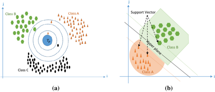
Machine learning classifiers (a) KNN, (b) SVM
The shape of the data is 900 row and 4 columns. The rows represent the number of samples while the 4 columns represent the 4 features. The 900 samples contain 300 data points for each class of EDW, MD and MDW codes. The 300 data points for each class are split into training and test data. The training set is 200 samples for each class while the test set is 100 data points for each class. The 4 columns consist of the predictors and the output label. The predictors are Q-factor, BER and SNR while the fourth column is the label (output). The label is categorized as EDW, MD, and MDW. The training set is used for both KNN and SVM classifiers for model training. Then, the test set is used for model evaluation.

4 Results and discussion
In this section, we present the obtained simulation results and ML classification results.
4.1 Simulation results
Here, we present the obtained simulation results that are conducted through Optisystem ver. 18, using the parameters given in Table 3 (Sarangal et al. 2021a, b; Abd El-Mottaleb et al. 2021).
The obtained number of chips that reach the PHD, Wh, for each case, is as follows.
Wh = 3 for MD code as there is no interference between users so at the receiver, decoder has the same spectral of the encoder and that is equal to W = 3.
Wh = 1 for EDW code as the decoder has only the non-interference bits that are equal to W − 2 = 3 − 2 = 1.
Wh = 2 for MDW code as the decoder has only the non-interference bits that are equal to (W/2) = (4/2) = 2.
Figure 4 illustrates the impact of different CA, LM, VLF, and LF conditions, respectively, on the proposed FSO system performance in terms of BER. Clearly, a longer propagation range can be achieved when EDW code is used with log(BER) less than − 3 under various weather scenarios. Ranges of 7, 3.5, 1.8, and 0.98 km, respectively, with log (BER) values − 5, − 7.2, − 7.9 and − 6.7, respectively, are achieved under CA, LM, VLF and LF, respectively. While, when MD code is used, minimum propagation distances can be achieved; 6.3, 3.2, 1.7, and 0.92 km with log(BER) less than − 3. As expected, when the range between transmitter and receiver increases, the BER decreases and the VLF condition gives the worst performance for all the codes while LM gives moderate performance and the best performance is CA.

Log(BER) versus propagation range under: (a) CA, (b) LM, (c) VLF, (d) LF
Figure 5 shows the relation between the Q-factor and propagation distance for different codes under different weather scenarios. As expected, as the distance between transmitter and receiver increases, the Q-factor decreases and the FSO communication system that uses EDW code gives the best value of Q-factor for higher propagation range which is 9.1, 7.1, 5.5 and 5, respectively for ranges 5.5, 3.2, 1.8 and 0.98 km, under CA, LM, VLF and LF, respectively. The system that uses MD code gives the worst performance at a longer propagation range. Also, the three systems can propagate longer distances under CA while a shorter range is obtained under VLF due to the attenuation that occurs under this weather condition and causes signal degradation.

Q-factor versus propagation range under: (a) CA, (b) LM, (c) VLF, (d) LF
Figure 6 displays the received power for different FSO systems that use EDW code with a code weight of 3, MDW code with a code weight of 4 and MD code with a code weight of 3 for three users versus the propagation range. For a shorter range between transmitter and receiver, higher received power is obtained and it degrades with increasing the range. Both EDW and MDW codes achieve a received power higher than MD code. The obtained received power at 5.5 km under CA for EDW, MDW and MD codes is, respectively, − 21.58, − 22.04 and − 23.8 dBm. While under the LM condition, the received power is − 22.7, − 23.18 and − 24.9 dBm for EDW, MDW and MD codes, respectively, at a propagation distance of 3.2 km. The received powers for EDW code as well as MDW code under VLF are − 23.8 and − 24.3 dBm, respectively, at 1.9 km and a BER less than \({10}^{-9}\) while for MD code, its received power at the same distance is − 26.08 with BER greater than 10–9. So, this system cannot be used for longer propagation distances. Under the LF condition, to make the three systems that use three different codes propagate with achievable received power that corresponds to log (BER) less than -2.5, it is preferred to take the propagation link 0.92 km.

Received power versus propagation range under: (a) CA, (b) LM, (c) VLF, (d) LF
Table 4 summarizes the received power for the different codes under CA, LM, VLF, and LF, at 5.5, 3.2, 1.9, and 0.92 km propagation range, respectively.
Figure 7 reports the SNR with the propagation range under various weather scenarios and different codes. As the propagation distance between transmitter and receiver increases, the SNR increases and the three systems give the best value for SNR under CA weather, while the worst value occurs under VLF, as expected. The system that uses EDW code gives the best value of SNR as declared from Fig. 7, which is 7.62, 5.3, 3, and 2.2 dB, at 5.5, 3.2, 1.9, and 0.98 km, respectively, under CA, LM, VLF and LF, respectively.

SNR versus propagation range under: (a) CA, (b) LM, (c) VLF, (d) LF
4.2 ML results
In this part, we will display and discuss the obtained ML results. The KNN and SVM results are displayed in Figs. 8 and 9, respectively, for each weather condition. When the color of the diagonal cells is biased toward yellow, this indicates high classification accuracy.

Confusion matrices of KNN classifier in code prediction under: (a) CA, (b) LM, (c) VLF, (d) LF

Confusion matrices of SVM classifier in code prediction under: (a) CA, (b) LM, (c) VLF, (d) LF
Since the software used in the classification task takes a random state of the data groups: EDW, MDW and MD, so, the number of test or training data may vary within 1%, for example, instead of using 100 data points for test. It takes 99 or 101 data points such as the case of EDW and MDW in confusion matrices in Figs. 8 and 9, respectively. Figure 8 displays the classification results of the KNN classifier, where the classification results of CA, LM and LF are reliable. The VLF case has the worst classification accuracy among the other cases. This is because of the distribution of the complex data in the VLF case. On the other hand, Fig. 9 is the visualization of SVM confusion matrices for each weather condition. The figure shows promising SVM classification results in CA, LM and LF but slightly less accurate than KNN. So, the KNN has better results than SVM. This is because, in this case, the distribution of the input dataset which is more adequate for KNN. Also, the worst classification accuracy case for the SVM is the same like the KNN classifier which is the VLF case. Table 5 shows the average and standard deviation of each parameter for the three codes under different weather conditions and the highest ML classification performance is achieved under the LM weather condition.
The two supervised learning algorithms are simple and efficient in terms of the computational time. As the number of neighbors, K, in the KNN algorithm increases, the complexity of computing decreases, but, in a trade-off with noise consideration. So, the K neighbors in the KNN is taken equal to 10 in order to reduce the computational complexity, showing good results. The Euclidian distance is the metric used in calculations. Moreover, the SVM with radial basis function (RBF) Kernel adopted shows also satisfying results. In CA, LM and LF, both classifiers show more than 97% of classification accuracy and in most cases. The KNN provides better results such as 99% accuracy since SVM requires less complexity than KNN. Also, in case of LF, both classifiers achieve 100% accuracy, i.e. highest precision and recall. However, many misclassifications may occur in some cases such as the VLF case since the accuracies are 82% and 81% for KNN and SVM, respectively. These misclassifications are due to the structure of the dataset in VLF and at certain cases, the SNR of MD code is 0. This is because of the distance range at which the measurements are taken according to the corresponding weather condition.
Since the accuracy is not enough to evaluate the model performance, so, other important performance evaluation parameters such as precision, recall and F1-score are adopted (Bansal and Singhrova 2021). These parameters are extracted from the statistical properties of the confusion matrix. The precision indicates the quality of a positive prediction provided by the algorithm. The recall is the number of true positives divided by the number of true positives plus the number of false negatives. The F1-score is a combination of recall and precision. Table 6 shows more of the ML evaluation parameters. In case of CA, both SVM and KNN show promising results in classifying the EDW, MD and MDW codes. The F1-score of SVM is 0.98, 0.98 and 1 for EDW, MD and MDW, respectively. The KNN shows exactly similar values like SVM. This indicates that the classification accuracy and performance for both algorithms in CA are reliable. The KNN outperforms the SVM in the case of LM, where the KNN shows a F1-score of 0.99, 0.99 and 1, while the SVM has a F1-score of 0.97, 0.95 and 0.98. In case of VLF, both algorithms show the worst classification performance since the F1-score 0.73 and 0.75 in MD for KNN and SVM, respectively. The LF case is ideal as both KNN and SVM achieve 100% precision, recall and F1-score. This indicates that the LF case has the best reliability of using KNN or SVM.
5 Conclusion
This paper proposes different SAC-OCDMA systems assigned three different codes; EDW, MDW, and MD codes based FSO communication. A coherent continuous wave laser source is used at the transmitter. A direct detection (DD) technique is used at the receiver for detecting the required user. The performance of the proposed systems is evaluated under different weather conditions: CA, LM, VLF, and LF in terms of Q-factor, bit error rate (BER), received power, and signal to noise ratio (SNR). Moreover, two machine learning (ML) algorithms, K-Nearest Neighbor (KNN) and Support Vector Machine (SVM), are used to classify the receiving code, whether it is EDW code, MDW code, or MD code. The conducted results reveal that the FSO communication system with the EDW code achieves the longest propagation distance with higher received power compared with the other codes; MDW and MD. It can transmit up to 7 km under CA, 3.5 km under LM, 1.8 km under VLF, and 0.8 km under LF with BER less than \({10}^{-6}\). The received power when the EDW code is used at a 5 km FSO link is − 21.58 dBm under CA, which is decreased to − 22.04 dBm and − 23 dBm when MDW and MD codes are used, respectively. Furthermore, the transmitting code (EDW, MDW, or MD) is translated into a classification issue from the perspective of ML by normalizing and employing the evaluation parameters (Q-factor, BER, and SNR) that are used as ML input features. Both ML algorithms, KNN and SVM, showed good classification between the three codes in most weather conditions in terms of accuracy, precision, and recall. They achieved 100% accuracy under LF while under VLF, the accuracy is 82% when the KNN algorithm is used and 81% when the SVM algorithm is used.
The enhancement of the classification of the VLF case should be considered as a future work. The VLF case must be studied from the perspective of the ML classifier. So, some preprocessing methods can be carried out, including cross-validation techniques. This step will most likely lead to better classification results during ML processes.
Data availability
The data used and/or analyzed during the current study are available from the corresponding author on reasonable request.
References
Abd, T.H., Aljunid, S.A., Fadhil, H.A., Ahmad, R.A., Saad, N.M.: Development of a new code family based on SAC-OCDMA system with large cardinality for OCDMA network. Opt. Fiber Technol. 17(4), 273–280 (2011)
Abd, T.H., Aljunid, S.A., Fadhil, H.A., Ahmad, R.B.A.: New algorithm for development of dynamic cyclic shift code for spectral amplitude coding optical code division multiple access systems. Fiber Integr. Opt. 31(6), 397–416 (2012)
Abd El-Mottaleb, S.A., Fayed, H.A., Abd El-Aziz, A., Metawee, M.A., Aly, M.H.: Enhanced spectral amplitude coding OCDMA system utilizing a single photodiode detection. J. Appl. Sci. 8(10), 1861–1874 (2018)
Abd El-Mottaleb, S.A., Fayed, H.A., Aly, M.H., Rizk, M.R.M., Ismail, N.: An efficient SAC-OCDMA system using three different codes with two different detection techniques for maximum allowable users. Opt. Quantum Electron. 51(11), 354–371 (2019)
Abd El-Mottaleb, S.A., Fayed, H.A., Aly, M.H., Rizk, M.R.M., Ismail, N.: MDW and EDW/DDW codes with AND subtraction/single photodiode detection for high performance hybrid SAC-OCDMA/OFDM system. Opt. Quantum Electr. 52(5), 239–259 (2020)
Abd El-Mottaleb, S.A., Métwalli, A., Hassib, M., Alfikky, A.A., Fayed, H.A., Aly, M.H.: SAC-OCDMA-FSO communication system under different weather conditions: Performance enhancement. Opt. Quantum Electron. 53(11), 616–633 (2021)
Abdualgalil, B., Abraham, S.: Applications of machine learning algorithms and performance comparison: a review. In: 2020 International Conference on Emerging Trends in Information Technology and Engineering (ic-ETITE), Vellora, India, pp. 1–6, 24–25 (2020)
Aggarwal, V., Gupta, V., Singh, P., Sharma, K., Sharma, N.: Detection of spatial outlier by using improved z-score test. In: 2019 3rd International Conference on Trends in Electronics and Informatics (ICOEI), Tirunelveli, India, pp. 788–790 (2019)
Aldhaibani, A.O., Aljunid, S.A., Fadhil, H.A., Anuar, M.S.: Performance analysis of hybrid OFDM/SAC-OCDMA systems based on MD code. J. Jokull 63(9), 34–44 (2013)
Aljunid, S.A., Ismail, M., Ramli, A.R., Ali, B.M., Abdullah, M.K.: A new family of optical code sequences for spectral-amplitude coding optical CDMA systems. IEEE Photonics Technol. Lett. 16(10), 2383–2385 (2004)
Al-Khafaji, H.M.R., Aljunid, S.A., Fadhil, H.A.: Improved BER based on intensity noise alleviation using developed detection techniques for incoherent SAC-OCDMA systems. J. Mod. Opt. 59(10), 878–886 (2012)
Angra, S., Ahuja, S.: Machine learning and its applications: a review. In: 2017 International Conference on Big Data Analytics and Computational Intelligence (ICBDAC), Cirala, Audhra, India, pp. 57–60 (2017)
Anuar, M.S., AlJunid, S.A., Arief, A.R., Junita, M.N., Saad, N.M.: PIN versus avalanche photodiode gain optimization in zero cross correlation optical code division multiple access system. Optik 124(4), 371–375 (2013)
Bansal, A., Singhrova, A.: Performance analysis of supervised machine learning algorithms for diabetes and breast cancer dataset. In: Proceeding of the 2021 International Conference on Artificial Intelligence and Smart Systems (ICAIS), Coimbatore, India, pp. 137–143 (2021)
Chaudhary, S., Amphawan, A., Nisar, K.S.: Realization of free space optics with OFDM under atmospheric turbulence. Optik 125(18), 5196–5198 (2014)
Dimitrov, S., Haas, H.: Information rate of OFDM-based optical wireless communication systems with nonlinear distortion. J. Light. Technol. 31(6), 918–929 (2013)
Fadhil, H.A., Aljunid, S.A., Ahmad, R.B.: Performance of random diagonal code for OCDMA systems using new spectral direct detection technique. Opt. Fiber Technol. 15(3), 283–289 (2009)
Fadhil, H.A., Amphawan, A., Shamsuddin, H.A.B., Abd, T.H., Al-Khafaji, H.M.R., Aljunid, S.A., Ahmed, N.: Optimization of free space optics parameters: an optimum solution for bad weather conditions. Optik 124(19), 3969–3973 (2013)
Hwang, C. -P., Chen, M. -S., C. Shih, C. -M., Chen, H. -Y., Liu, W. K.: Apply scikit-learn in python to analyze driver behavior based on OBD data. In: 2018 32nd International Conference on Advanced Information Networking and Applications Workshops (WAINA), Krakow, Poland, pp. 636–639 (2018)
Karpagarajesh, G., SanthanaKrishnan, R.S., Obinson, Y.H., Vimal, S., Kadry, S., Nam, Y.: Investigation of digital video broadcasting application employing the modulation formats like QAM and PSK using OWC, FSO, and LOS-FSO channels. Alex. Eng. J. 61(1), 647–657 (2022)
Kaur, J., Khan, M.A., Iftikhar, M., Imran, M., Ul Haq, Q.E.: Machine learning techniques for 5G and beyond. IEEE Access. 9, 23472–23488 (2021)
Khalighi, M.A., Uysal, M.: Survey on free space optical communication: a communication theory perspective. IEEE Commun. Surv. Tutor. 16(4), 2231–2258 (2014)
Kolev, D.R., Wakamori, K., Matsumoto, M.: Transmission analysis of OFDM-based services over line-of-sight indoor infrared laser wireless links. J. Light. Technol. 30(23), 3727–3735 (2012)
Mirza, J., Imtiaz, W., Ghafoor, S.A.: Integrating ultra-wideband and free space optical communication for realizing a secure and high throughput body area network architecture based on optical code division multiple access. Opt. Rev. 28(5), 525–537 (2021)
Moghaddasi, M., Mamdoohi, G., Noor, A.S.M., Mahdi, M.A., Anas, S.B.A.: Development of SAC-OCDMA in FSO with multi-wavelength laser source. Opt. Commun. 356, 282–289 (2015)
Moghaddasi, M., Mamdoohi, G., Noor, A.S.M., Mahdi, M.A., Anas, S.B.A.: Evaluation of optical code division multiple access (OCDMA) encoding techniques for free space optics (FSO). Lasers Eng. 33(4), 247–260 (2016)
Moghaddasi, M., Seyedzadeh, S., Glesk, I., Lakshminarayana, G., Anas, S.B.A.: DW- ZCC code based on SAC-OCDMA deploying multi-wavelength laser source for wireless optical networks. Opt. Quantum Electron. 49(12), 393–406 (2017)
Mostafa, S., Mohamed, A.E.-N.A., El-Samie, F.E.A., Rashed, A.N.Z.: Performance evaluation of SAC-OCDMA system in free space optics and optical fiber system based on different types of codes. Wirel. Pers. Commun. 96(2), 2843–2861 (2017)
Palais, J.C.: Fiber Optic Communications, 5th edn. Upper Saddle River, Pearson Prentice Hall, NJ (2005)
Robinson, S., Jasmine, S.: Performance analysis of hybrid WDM-FSO system under various weather conditions. Frequenz 70, 9433–9441 (2016)
Sahbudin, R.K.Z., Abdullah, M.K., Mokhta, M.: Performance improvement of hybrid subcarrier multiplexing optical spectrum code division multiplexing system using spectral direct decoding detection technique. J. Opt. Fiber Technol. 15(3), 266–273 (2009)
Sarangal, H., Singh, A., Malhotra, J., Chaudhary, S.: A cost effective 100 Gbps hybrid MDM–OCDMA–FSO transmission system under atmospheric turbulences. Opt. Quantum Electron. 49(5), 184–193 (2017)
Sarangal, H., Nisar, K.S., Thapar, S.S., Singh, A., Malhotra, J.: Performance evaluation of 120 GB/s hybrid FSO-SACOCDMA-MDM system using newly designed ITM-Zero cross-correlation code. Opt. Quantum Electron. 53(1), 64–75 (2021a)
Sarangal, H., Singh, A., Malhotra, J., Thapar, S.S.: Performance Investigation of PM-ZCC Code in Hybrid SAC-OCDMA System through Inter-Satellite OWC Channel. Wirel. Pers. Commun. 120(4), 3329–3341 (2021b)
Singh, M., Malhotra, J.: Long-reach high-capacity hybrid MDM-OFDM-FSO transmission link under the effect of atmospheric turbulence. Wirel. Pers. Commun. 107(4), 1549–1571 (2019)
Wei, Z., Shalaby, H.M.H., Ghafouri-Shiraz, H.: Modified quadratic congruence codes for fiber Bragg-grating-based spectral-amplitude-coding optical CDMA systems. J. Light. Technol. 19(9), 1274–1281 (2001)
Zhang, J., Liu, L., Fan, Y., Zhuang, L., Zhou, T., Piao, Z.: Wireless channel propagation scenarios identification: A perspective of machine learning. IEEE Access. 8, 47797–47806 (2020)
Funding
Open access funding provided by The Science, Technology & Innovation Funding Authority (STDF) in cooperation with The Egyptian Knowledge Bank (EKB). The authors did not receive any funds to support this research.
Author information
Authors and Affiliations
Contributions
S.A.A., A.M., M.S., M.H., M.H.A. have directly participated in the planning, execution, and analysis of this study. AHB drafted the manuscript. All authors have read and approved the final version of the manuscript.
Corresponding author
Ethics declarations
Conflict of interest
The authors declare that they have no competing interests.
Ethical approval
Not Applicable.
Additional information
Publisher's Note
Springer Nature remains neutral with regard to jurisdictional claims in published maps and institutional affiliations.
OSA member: Moustafa H. Aly.
Rights and permissions
Open Access This article is licensed under a Creative Commons Attribution 4.0 International License, which permits use, sharing, adaptation, distribution and reproduction in any medium or format, as long as you give appropriate credit to the original author(s) and the source, provide a link to the Creative Commons licence, and indicate if changes were made. The images or other third party material in this article are included in the article's Creative Commons licence, unless indicated otherwise in a credit line to the material. If material is not included in the article's Creative Commons licence and your intended use is not permitted by statutory regulation or exceeds the permitted use, you will need to obtain permission directly from the copyright holder. To view a copy of this licence, visit http://creativecommons.org/licenses/by/4.0/.
About this article

Cite this article
Abd El-Mottaleb, S.A., Mètwalli, A., Singh, M. et al. Machine learning FSO-SAC-OCDMA code recognition under different weather conditions. Opt Quant Electron 54, 851 (2022). https://doi.org/10.1007/s11082-022-04223-4
Received:
Accepted:
Published:
DOI: https://doi.org/10.1007/s11082-022-04223-4