
Abstract
In this paper, we consider cooperative manipulation of a planar rigid body using multiple actuator agents—unilateral thrusters, each attached to the body and each able to apply an unilateral force to the body. Generally, the dynamics of the body manipulated with uncoordinated forces of thrusters is nonlinear. The problem we consider is how to design the unilateral force each agent applies to ensure the decoupling and linearity of the linear and angular (i.e., translational and rotational) accelerations of the body and thus allow a controller to be designed in a simpler manner, instead of developing sophisticated nonlinear control techniques. Here consider two types of unilateral thrusters with (i) all fixed directions, and (ii) all non-fixed directions, respectively. To address the problem, we design two decomposition frameworks, each with its advantages, on the structure of the forces and control policy such that (i) the linear and angular accelerations of the body are decoupled and controlled independently, and (ii) the control that ensures the forces to be unilateral (only for thrusters with non-fixed directions) is independent from the linear and angular accelerations. As a result, the closed-loop dynamics of the body is linear with respect to both the linear and angular accelerations; thus the control of the body becomes trivial, which may provide a convenient and alternative methodology for design of a physical system with a quick estimation and reference of the manipulated forces required.
1 Introduction
Cooperative manipulation or transportation of multiple agents is often seen in natural world [1, 2] and artificial world [3–6]. In this paper, we consider the problem of controlling a planar rigid body through the interaction forces applied by multiple attached actuators or thrusters. The manipulation of a rigid body using multiple thrusters or mobile robotic agents is a challenging problem with a number of applications. For example, tethered towing [7–9], grasping [10–12], pushing and caging [13, 14], satellite control with thrusters [15], object transportation [14], and other problems all can be made to fit within the paradigm of cooperative manipulation.
Manipulation and/or transportation of a rigid body has been investigated by many researchers. Lynch and Mason investigated the non-prehensile manipulation in [16]. Lynch investigated controllability of a rigid body with the minimal number of unilateral thrusters [15]. Spong [17] and Partridge and Spong [18] investigated control of a rigid body with impacts, i.e., impulsive manipulation. Forni, etc., considered tracking and state-estimation of a bouncing ball with impacts [19]. In [13, 15–19], the rigid body is controlled by applying unilateral forces. The object transportation by the “object closure” of multiple ground robots was investigated in [14], and transportation of a payload by multiple aerial robots was considered in [7, 8]. Esposito [20] considered control of a rigid body with lateral forces of attached robots for velocity tracking and followed by an “approach” (i.e., agents approach to the perimeter of the body) investigated in [21].
Generally, the type of the forces of agents applied to the manipulated rigid body can be (i) all bilateral, or (ii) all unilateral or (iii) the mixed (i.e., some forces applied are bilateral while others are unilateral). To be specific, a bilateral force on the body can be pull or push, but at different time in the manipulation process, while a unilateral force, applied through unilateral contact, can be either pull or push, at all the time, without switch between pull or push. The zero force is trivial and can be regarded as either a bilateral force or an unilateral pull or push force. Additionally, the unilateral forces of multiple thrusters can be divided into three categories: (1) The forces are all pull at all the time, for example, when tethered towing or using the unilateral thrusters directed to the outer of the body; (2) the forces are all push at all the time, for example, when grasping or pushing or using the unilateral thrusters directed to the inner of the body; (3) the mixed, i.e., some forces are pull and others are push. Following the scenarios of multi-actuator or multi-thruster manipulation, we consider the cooperative manipulation of a planar rigid body with multiple unilateral thrusters that are attached to the body. The directions of the thrusters (i.e., the directions of the applied forces) can be all fixed or swing, and the forces generated by the thrusters are unilateral, either all pull or all push, on the body.
Generally, a rigid body has nonlinear translation and rotation dynamics when manipulated with uncoordinated forces and thus is not easily made small-time locally controllable (STLC) [15], and the design of the forces for certain tasks (e.g., trajectory tracking of the rigid body) may be complex.
In contrast to previous work on the manipulation and transportation methodologies mentioned above, the main contributions of this paper are summarized as follows: (1) We consider two types of the attached unilateral thrusters to the body for the manipulation, i.e., the thrusters with (i) all fixed directions and (ii) all non-fixed (i.e., swing) directions, respectively. (2) In this context of the unilateral-thruster-control, we aim to control the body that is easily STLC, and as a result, the rigid body can easily achieve the desired trajectory of the configuration (i.e., position and orientation states) of the rigid body, not merely to transport it to a target location, as compared with the object transportation mentioned above. (3) Moreover, we aim to develop two decomposition frameworks, each of which allows the controllers for translational control and rotational control that can be designed separately and trivially, with a unified control policy of the forces for either all pull or all push, which may provide a convenient and alternative methodology for design of a physical system with a quick estimation of the manipulated forces required.
To achieve these results, we emphasize (i) how to design the forces applied to the body to be all unilateral in the manipulation? and (ii) how to ensure the linear and angular (i.e., translational and rotational) accelerations of the body to be decoupled and linear? Item (i) is for the physical constraint of unilateral thrusters. For Item (ii), if it can be achieved, then the rigid body is STLC and thus can be easily controlled which provides much convenience for designing control laws.
This paper considers two decomposition frameworks that are denoted as Frameworks I and II, each with its advantages, on the structure of the forces and control policy.
In Framework I: for attached thrusters with all fixed directions, we arrange the thrusters into two categories with heterogeneous roles: One category is for pure translational control and has no influence on the rotational dynamics of the body; another is for pure rotational control and has no influence on the translational dynamics of the body. As an example, we design the control policy of the thrusters for rotational control in an alternative working manner to ensure the desired trajectory tracking of the body. In this case, the framework is efficient in the sense that, for a large number of thrusters, there is less portion of force canceling effect, but the workload for individual thrusters may be not balanced depending on what type of trajectory tracking.
In Framework II: for the attached thrusters with all non-fixed directions, based on the proper attached locations of the thrusters, we design the applied force of every thruster with threefold decomposition terms, each with a different role, to control (i) rotation and (ii) translation and (iii) the overall applied force to be unilateral, respectively, and without coupling. To be specific, for the threefold decomposition terms of all forces: (1) the components of the forces that control rotation of the body are balanced, i.e., the composition of these forces’ components is zero, and consequently, they have no influence on translation of the body; (2) the components of the forces that control translation of the body have balanced moments, i.e., the composition of the moments of the forces is zero so that they have no influence on rotation of the body; (3) the components of the third structure are used to make the forces to be all unilateral (pull or push), which are balanced with balanced moments, and thus have no influence on the rotation and translation of the body. Moreover, under this framework, the control policy for pull or push is unified, i.e., it has the same mathematical form for pull or push and can be easily switched, and the closed-loop dynamics of the body is linear with respect to both rotation and translation. Examples are given to illustrate the notions. In this framework, the workload for individual thrusters is generally roughly balanced, but it is less efficient in the sense that there may be a larger portion of force canceling effect than the case in Framework I.
Although in Framework II, the perfect placement of the thrusters is required, this framework nevertheless provides many useful insights for controlling a rigid body in a simple and linear formulation such that the rigid body is easily STLC and easily implemented, as opposed to developing possibly sophisticated nonlinear control techniques which are not easy to satisfy both the unilateral restriction and the STLC requirement together with easy implementation. The possible non-perfect placement of thrusters in physical applications is not unsolvable, either by a careful calibration of the placement or compensation (possibly by an additional thruster that will be investigated). Some future considerations (e.g., the compensation of non-perfect placement, as well as inaccurate measurements, fuel consumption of thrusters, etc.) are listed in Conclusion.
The remainder of the paper is organized as follows. Section 2 is the problem description. Section 3 is the assumptions and definitions. Section 4 is the control design of unilateral thrusters with fixed directions, with examples given in Sect. 5. Section 6 designs the framework on the structure of the forces and the control policy for the thrusters with non-fixed directions. As a result, the control of the rigid body in each of the frameworks becomes trivial, as examples illustrated in Sect. 7. Section 8 is the conclusion and suggestions for possible future work. Table 1 lists some notations used in this paper for convenience of reference.
2 Problem description
2.1 Manipulation of rigid body
Consider the \(n\) unilateral thrusters attached to a planar rigid body in the two-dimensional Euclidean space [15, 20], as shown in Fig. 1, the directions of the thrusters can be all fixed or all swing, with the constraints that all the thrusters direct to the outer or inner of the body (i.e., the thrusters can only apply pull or push forces to the body). Assume that a body-fixed reference frame is attached to the mass center of the body and we denote by \(x(t) \in \mathbb {R}^2\) and \(R(\psi (t))\in SO(2)\) the position, respectively, orientation of the body in an inertial frame, \(\psi (t)\in \mathbb {R}\). Without loss of generality, assume the body-fixed frame has its initial orientation as the inertial frame, i.e., \(\psi (0)=0\). The linear and angular velocities of the body are denoted as \(\dot{x}(t)\) and \(\dot{\psi }(t)\), respectively. Then, the dynamics of the body can be described by the equations in the inertial frame:
where \(m\) is the mass of the bodyFootnote 1 and \(I\) is the moment of inertia about the mass center of the body; \(f_k(t)\in \mathbb {R}^2\) and \(M_k(t)\in \mathbb {R}\) are the force and moment of thruster \(k\) applied to the body, respectively, and since the body is on the plane, here for simplicity, we denote the moment \(M_k(t)\) as a scalar and denote \(M_k(t)>0\) when it generates angular acceleration on the body counterclockwise, with its magnitude defined as
where \(\times \) means the cross product, \(\tilde{r}_k\in \mathbb {R}^2\) is the location vector that from the mass center to the attached location of agent \(k\) in the body-fixed frame and thus is a constant, \(|\cdot |\) and \(||\cdot ||\) represent the absolute value of a scalar and the norm of a vector, respectively. The rotation matrix \(R(\cdot )\) is defined as follows:
where \(\theta \in \mathbb {R}\) is the parameter of the rotation matrix.

Illustration of the manipulation of a planar rigid body, the circles represent the thrusters attached to the rigid body, the dotted arrows denote the forces on the body generated by the thrusters
The dynamics Eqs. (1) and (2) of the rigid body is generally nonlinear with uncoordinated control forces, with its linear and angular (i.e., translational and rotational) accelerations coupled, which make the rigid body not STLC and the control not easy.
2.2 Notations in the body-fixed and inertial frames
There are two reference frames, i.e., the body-fixed frame and the inertial frame. In this paper, express a variable with a tilde when in the body-fixed frame, and express the corresponding variable without a tilde in the inertial frame. For example, \(\tilde{f}_k(t)\) is the applied force \(f_k(t)\) of thruster \(k\) when expressed in the body-fixed frame; the constant location vector \(\tilde{r}_k\), when viewed in the initial frame, is a variable, denoted as \(r_k(\psi (t))\), where \(r_k(\psi (t))= R(\psi )\tilde{r}_k\).
2.3 Definitions of unilateral forces
Definition 1
Thruster \(k\) attached to the perimeter of the body applies a pull force to the body if
(notation \(\cdot \) means the dot product) and a push force if
where \(\tilde{n}_k \in \mathbb {R}^2\) is the normal vector of the perimeter of the body at location of agents \(k\) in the body-fixed frame, as illustrated in Fig. 2.

Illustration of the unilateral force on the body. \(\tilde{n}_k\) is the norm vector of the perimeter of the body at the location of agent \(k\)
2.4 Main Considerations
In this paper, we consider the problem: how to design a framework and the forces of the thrusters to achieve that
-
(1)
the forces are unilateral and the rigid body is STLC with \(n\ge 2\) (note that it is not STLC with only one thruster),Footnote 2 moreover
-
(2)
the linear and angular accelerations of the body are decoupled and controlled independently,
-
(3)
the control that ensures the forces to be unilateral is independent from the linear and angular accelerations, and
-
(4)
the closed-loop dynamics of the body is linear with respect to both the linear and angular accelerations (which implies that the body is STLC).
As a result, the rigid body can be easily controlled and the design of control laws for manipulation becomes trivial.
3 Assumptions and definitions
3.1 Assumptions
For the shape of the body at the attached locations, since we need to parametrize the attachment location by an angle, we assume the shape of the body is diffeomorphic to a circle (although for simplicity, in the following figures, the shape of the body is illustrated as a circle). Denote \(\vartheta _k\) as the angle between the norm vector \(\tilde{n}_k\) and the location vector \(\tilde{r}_k\), then
as illustrated in Fig. 2.
Remark 1
For a special case, when the body’s shape is a regular circle with the mass center at the center of the body, then \(\vartheta _k=0\) for all agents \(k\).
3.2 Definitions
Denote \(0\le \tilde{\theta }_k<2\pi \) as the attached angle of thruster \(k\) in the body-fixed frame.
Definition 2
(Placement of the thrusters that positively span the plane): For the placement of the \(n\) thrusters that positively span the plane, we mean that the angles \(\tilde{\theta }_k, k=1,2,\ldots ,n\), are distributed more or less uniformly, with
where the notion \(\text {i}=\sqrt{-1}\) means the imaginary unit.
Definition 3
The perfect placement of the thrusters is that: the angles \(\tilde{\theta }_k, k=1,2,\ldots ,n\), are distributed more or less uniformly, with
Remark 2
Note that when \(n>3\), the perfect placement of the thrusters does not necessarily mean their angles \(\tilde{\theta }_k\), \(k=1,2,\ldots ,n\), are uniformly distributed on the circle. For example, when \(n=4, \tilde{\theta }_1=0\), \(\tilde{\theta }_2=2\pi /3, \tilde{\theta }_3=\pi \), \(\tilde{\theta }_4=5\pi /3\).
Remark 3
Figure 3 illustrates the positively-spanning-placement (Definition 2) and the perfect placement (Definition 3).

Illustration of the placement of the thrusters attached to a rigid body, the circles represent the thrusters attached on the rigid body, for simplicity, assume the shape of the rigid body is a circle, the mass center is at the center of the circle. (i) The thrusters positively span the plane. (ii) The thrusters do not positively span the plane. (iii) The uniformly perfect placement of the thrusters
Remark 4
To derive one instance of each of the \(n\) values for two placements defined above, one may use, for example, the protocol of Proposition 6 in [22] which convergence is asymptotic. Then one instance of the \(n\) values of the angles in Definition 3 (or Definition 2) is then derived, if the protocol in Proposition 6 in [22] is allowed to converge sufficiently (or the evolution of the protocol is just interrupted before sufficient convergence).
Remark 5
The positively-spanning-placement allows the thrusters located in a more general configuration and is thus a mild assumption. The constraint of the perfect placement (e.g., condition (8) can be achieved by simply assigning \(\tilde{\theta }_k=\phi _0+\frac{(k-1)2\pi }{n_k}, k=1,2,\ldots ,n\), \(\phi _0\in \mathbb {R}\)) is rigorous and will provide much convenience in the design of the controller; however, this is likely not possible to do perfectly in physical systems, but through careful calibration, the error can be made neglected in application.
4 Decomposition framework and control design of unilateral thrusters with fixed directions
Considering the \(n\ge 5\) unilateral thrusters attached to the rigid body with all fixed directions, this section designs the attached directions and the magnitudes of the applied forces of the thrusters. Without loss of generality, here assume the thrusters apply only pull forces on the body. (Note that, for the \(n\le 3\) unilateral thrusters with all fixed directions, the body cannot be STLC, which is implied in [15]. For \(n=4\), it is less likely feasible in this framework.)
In this section, divide the thrusters into two categories with:
where
-
the \(n_t\) thrusters are used for translational control, with the placement of the thrusters on the perimeter of the body that positively span the plane, \(n_t\ge 3\), the directions of the thrusters point out of the body and pass through the mass center, thus with no influence on the rotation of the body, and
-
the \(n_r\) thrusters are used for rotational control and form \(\frac{n_r}{2}\) couples with zero net force which have no influence on the translation of the body, where \(n_r\ge 2\) is an even number.
Without loss of generality, we number the \(n_t\) thrusters as \(1,2,\ldots ,n_t\) counterclockwise.
4.1 Thrusters for translational control
Assume \(f_r(t)\in \mathbb {R}^2\) is an arbitrary reference force in the inertial frame:
where \(c(t)\ge 0\) and \(\theta (t)\in \mathbb {R}\) are the magnitude and orientation (in the inertial frame) of the force \(f_r(t)\), respectively. Thus the force \(f_r(t)\) in the body-fixed frame, denoted as \(\tilde{f}_r(t)\), has the orientation \(\theta (t)-\psi (t)\).
For the \(n_t\) thrusters and current orientation \(\psi (t)\) of the rigid body, the direction of the thruster \(k\) is \(\psi (t)+\tilde{\theta }_k\) in the inertial frame, \(k=1,2,\ldots ,n_t\). Denote the magnitude of the force (i.e., one of the control inputs, since the directions are fixed) of the thruster \(k\) as \(c_k(t)\ge 0, k=1,2,\ldots ,n_t\). In the following, we design \(c_k(t)\) such that
in the inertial frame, or equivalently,
in the body-fixed frame.
Note that \(\theta (t)-\psi (t)\) is the direction of force \(R(-\psi (t)) f_r(t)\) in the body-fixed reference frame. To achieve constraint (11), just select two adjacent thrusters \(k\) and \(k+1\) at current state in the body-fixed reference frame, such that
where \(\hbox {mod}(\cdot ,\cdot )\) is the modulus function. The selection is illustrated in Fig. 4. The interval \([\tilde{\theta }_k, \tilde{\theta }_{k+1})\) with \(k=n_t\) means the interval \([\tilde{\theta }_{n_t}-2\pi , \tilde{\theta }_{1})\). For simplicity, denote the left term of (12) as
Proposition 1
Select \(k,k+1\) using the rule (12), and let
where
Then, the composition of the forces of thrusters \(k\) and \(k+1\) is \(f_r(t)\), and all other thrusters apply no forces, thus (11) holds.
Remark 6
Note that if \(\vartheta (t)=\tilde{\theta }_k\) at current time \(t\), then from Proposition 1, one can easily get:
as \(\vartheta (t)\rightarrow \tilde{\theta }_{k+1}\), then
Proof of Proposition 1
\(c_k(t)\) and \(c_{k+1}(t)\) are computed from the following two equations (refer to Fig. 4):
Then, we have
the above results hold.\(\square \)

Illustration of the magnitudes and angles in the body-fixed frame
Remark 7
The \(n_t\) thrusters are designed to work in an alternative manner, refer to Fig. 7.
Remark 8
The larger number \(n_t\) of the thrusters used for translation means that the difference of \(\tilde{\theta }_{k+1}-\tilde{\theta }_k\) generally decreases, and thus the more efficiency of the forces of the working thrusters (since the canceling effect of the working thrusters decreases).
4.2 Thrusters for rotational control
For the \(n_r\) thrusters, \(n_r\) is an even number, \(n_r\ge 2\), we place them as \(\frac{n_r}{2}\) couples, as illustrated in Fig. 5, the thrusters in each couple have parallel but opposite direction, and the distance is denoted as \(d_1,d_2,\ldots ,d_{\frac{n_r}{2}}>0\), respectively, in each couple of the thrusters. For simplicity, assume all \(n_r\) thrusters exert the forces with the same magnitude \(\alpha (t)\ge 0\). Then, the overall moment of the \(n_r\) thrusters on the body is \((d_1+d_2+\cdots +d_{\frac{n_r}{2}})\alpha (t)\), which controls the body in counterclockwise (for additional clockwise acceleration control, simply reverse the directions of one or more couples of unilateral thrusters or use bilateral thrusters which is trivial and omitted here).

Illustration of the \(\frac{n_r}{2}\) couples of the thrusters. The two thrusters in each couple have parallel but opposite direction, the distance is denoted as \(d_1,d_2,\ldots ,d_{\frac{n_r}{2}}>0\), respectively, in each couple of the thrusters
4.3 Dynamics of rigid body
It follows immediately from the above analysis that the dynamics (1)–(2) of the body reduce to
5 Examples for thrusters with fixed directions
Assume the desired trajectories of the body are given by \(x_d(t)\) and \(\psi _d(t)\) (in this section, for clarity, \(x_d(t), x(t)\), \(\psi _d(t)\) and \(\psi (t)\) are abbreviated as \(x_d, x, \psi _d\) and \(\psi \), respectively).
5.1 Pure translational control
For the pure translation of the rigid body, assume \(m{=}1\),
The initial condition: \(x(0)=[0.4,-0.2]^T, \dot{x}(0)=\mathbf {0}\). Let:
then \(x(t)\rightarrow x_d(t), \dot{x}(t)\rightarrow \dot{x}_d(t)\).
Assume there are \(n_t=4\) thrusters with the attached angles \(\tilde{\theta }_1=0, \tilde{\theta }_2=\frac{2}{3}\pi \), \(\tilde{\theta }_3=\pi , \tilde{\theta }_4=\frac{5}{3}\pi \) in the body-fixed frame. When \(k_p=k_d=1\), the dynamics of the body and \(f_r(t)\) are illustrated in Fig. 6. The applied forces \(c_k(t), k=1,2,3,4\), of the thrusters are illustrated in Fig. 7, with initial orientation \(\psi (0)=0\) and \(\psi (0)=-\frac{\pi }{4}\), respectively. The thrusters work in an alternative manner.

Illustration of dynamics of the rigid body and \(f_r(t)\) in the inertial frame, respectively, in the \(x-y\) plane

Illustration of magnitudes of the forces (the control inputs) \(c_k(t), k=1,2,3,4\), of the thrusters, with \(\psi (0)=0\) and \(\psi (0)=-\frac{\pi }{4}\), respectively
5.2 Both translational and rotational control
Assume \(m=1, I=1\),
The initial condition: \(x(0)=[0.4,-0.2]^T, \dot{x}(0)=\mathbf {0}\), \(\psi (0)=-\frac{\pi }{4}, \dot{\psi }(0)=0\). \(f_r(t)\) is given in (18) with \(k_p=k_d=1\).
Assume there are \(n_t=4\) thrusters with the attached angles \(\tilde{\theta }_1=0, \tilde{\theta }_2=\frac{2}{3}\pi \), \(\tilde{\theta }_3=\pi , \tilde{\theta }_4=\frac{5}{3}\pi \) in the body-fixed frame four translational control (as in Sect. 5.1), and another two thrusters for rotational control with \(d_1=1\), and
where \(\kappa _p,\kappa _d>0\). Then, \(x(t)\rightarrow x_d(t)\), \(\dot{x}(t)\rightarrow \dot{x}_d(t)\), and \(\psi (t)\rightarrow \psi _d(t), \dot{\psi }(t)\rightarrow \dot{\psi }_d(t)\). Figure 8 illustrates the dynamics of the configuration of the rigid body (\(\kappa _p=\kappa _d=1\)).

Dynamics of the rigid body in the \(x-y\) plane. The endpoint of each arrow denotes the mass center \(x(t)\) of the rigid body, with the direction of the arrow denotes \(\psi (t)\) or \(\dot{x}(t)\)
The magnitudes of the applied forces (the control inputs) are illustrated in Fig. 9, where \(\alpha (t)\) converges to zero, and \(c_3(t),c_4(t)\) converge to nonzero values, \(c_1(t)\) converges to zero, and \(c_2(t)\) is always zero.
6 Decomposition framework and control design of unilateral thrusters with non-fixed directions
In this section, we consider a decomposition framework and the unified control policy of unilateral thrusters with non-fixed directions. All the \(n\) thrusters are used to control both rotation and translation of the body, and in the meanwhile, to ensure the unilateral forces (all pull or all push) of all the thrusters.
In this section, \(n\ge 2\). Denote the attached location \(\tilde{r}_k=\ell _k [\cos \tilde{\theta }_k,\sin \tilde{\theta }_k]^T\) of thruster \(k=1,2,\ldots ,n\), in the body-fixed frame, here \(\ell _k:=||\tilde{r}_k||>0, \tilde{r}_k\) and \(\ell _k\) are determined by the shape of the body and attached angle of thruster \(k\). Generally, the attached location of each thruster is different from the location of the body’s mass center, thus \(\ell _k>0\), \(k=1,2,\ldots ,n\). Define the constant vector \(\varepsilon \in \mathbb {R}^2\) as follows:

Illustration of the magnitudes of the applied forces (the control inputs) of the thrusters \(\alpha (t)\), and \(c_k(t), k=1,2,3,4\)
6.1 Decomposition structure of applied forces
Design \(f_k(t)\) with the threefold decomposition terms:
where the superscripts “r, t, u” are the initial letters of “rotation, translation, unilateral,” respectively, as illustrated in Fig. 10.

Illustration of the decomposition of \(f_k(t)\) in the inertial frame
Denote the moments generated by the components of \(f^r_k(t)\), \(f^t_k(t), f^u_k(t)\) as \(M^r_k(t), M^t_k(t), M^u_k(t)\), respectively.
6.2 Control policy of applied forces
This section designs the structures of \(f_k^r(t)\) and \(f^u_k(t)\) in the body-fixed frame, that denoted as \(\tilde{f}_k^r(t)\) and \(\tilde{f}^u_k(t)\), respectively, while designs \(f_k^t(t)\) directly in the inertial frame.
-
(1)
Based on the locations of agents, simply specify \(\tilde{f}_k^r(t)\):
$$\begin{aligned} \tilde{f}_k^r(t)=a(t) R(\theta _0) \left( \begin{array}{c} \cos \tilde{\theta }_k \\ \sin \tilde{\theta }_k \\ \end{array} \right) , \end{aligned}$$where \(a(t)\in \mathbb {R}, 0<\theta _0<\pi \). \(\tilde{f}_k^r(t)\) generates positive moment (\(M_k(t)>0\)) on the body when \(a(t)>0\). For \(\theta _0=\frac{\pi }{2}, \tilde{f}_k^r(t)\) is most efficient for generating the moment since \(M^r_k(t) = a(t)\ell _k\sin (\theta _0)=a(t)\ell _k\), so in the following, we take \(\theta _0=\frac{\pi }{2}\), i.e.,
$$\begin{aligned} \tilde{f}_k^r(t)&= a(t)\left( \begin{array}{cc} 0 &{} -1 \\ 1 &{} 0 \\ \end{array} \right) \left( \begin{array}{c} \cos \tilde{\theta }_k \\ \sin \tilde{\theta }_k \\ \end{array} \right) ,\nonumber \\&k=1,2,\ldots ,n. \end{aligned}$$(21)In this case,
$$\begin{aligned} \sum _{k=1}^n \tilde{f}_k^r(t)&= a(t) \left( \begin{array}{cc} 0 &{} -1 \\ 1 &{} 0 \\ \end{array} \right) \varepsilon ,\\ \sum _{k=1}^n M^r_k(t)&= a(t) \sum _{k=1}^n \ell _k. \end{aligned}$$ -
(2)
Next choose the structure of the second force \(f_k^t(t)\)
$$\begin{aligned} f_k^t(t)=b_k g(t), ~ k=1,2,\ldots ,n \end{aligned}$$(22)in the inertial frame, where \(b_k\in \mathbb {R}\), and \(g(t)\in \mathbb {R}^2\) is an arbitrary reference force. The forces \(f_k^t(t), k=1,2,\ldots ,n\), are parallel. For the coefficient \(b_k\), considering the attached locations of the thrusters, simply select \(b_k\) to satisfy
$$\begin{aligned} b_k = 1 / \ell _k, \ k=1,2,\ldots ,n \end{aligned}$$(23)in which case,
$$\begin{aligned} \sum _{k=1}^n f_k^t(t)&= g(t) \sum _{k=1}^n \frac{1}{\ell _k},\\ \sum _{k=1}^n M^t_k(t)&= \sum _{k=1}^n f_k^t(t)\times R(\psi (t))\tilde{r}_k \\&= \sum _{k=1}^n g(t)\times R(\psi (t))\frac{\tilde{r}_k}{\ell _k} \\&= g(t)\times R(\psi (t)) \varepsilon . \end{aligned}$$ -
(3)
Design the structure of the force \(\tilde{f}^u_k(t)\) as follows:
$$\begin{aligned} \tilde{f}^u_k(t)= u(t) \left( \begin{array}{c} \cos \tilde{\theta }_k \\ \sin \tilde{\theta }_k \\ \end{array} \right) , \ k=1,2,\ldots ,n \end{aligned}$$(24)where \(u(t)\in \mathbb {R}\) is the unilateral control input, then \(\tilde{f}^u_k(t), k=1,2,\ldots ,n\), are almost balanced and have zero moments:
$$\begin{aligned} \sum _{k=1}^n \tilde{f}^u_k(t)&= u(t) \varepsilon ,\\ \sum _{k=1}^n M^u_k(t)&= \sum _{k=1}^n \tilde{f}^u_k(t) \times \tilde{r}_k = \mathbf {0}. \end{aligned}$$
In application, one can make a careful calibration of the perfect placement of the thrusters such that \(\varepsilon \approx \mathbf {0}\) can be neglected. Then, under this condition, these forces subject to the following three constraints:
-
(1)
the forces \(f_k^r(t), k=1,2,\ldots ,n\), are balanced, i.e.,
$$\begin{aligned} \sum _{k=1}^n f_k^r(t) = \mathbf {0} \end{aligned}$$(25)(these forces are used to control the rotation of the body),
-
(2)
\(f_k^t(t), k=1,2,\ldots ,n\), have balanced moments, i.e.,
$$\begin{aligned} \sum _{k=1}^n f_k^t(t) \times R(\psi (t))\tilde{r}_k =\mathbf {0} \end{aligned}$$(26)(these forces are used to control translation of the body),
-
(3)
\(f^u_k(t), k=1,2,\ldots ,n\), are balanced with balanced moments (thus for any control \(u(t)\), the dynamics of the body is unaffected), i.e.,
$$\begin{aligned} \sum _{k=1}^n f_k^u(t) = \mathbf {0}, \ \sum _{k=1}^n f_k^u(t) \times R(\psi (t))\tilde{r}_k =\mathbf {0} \end{aligned}$$(27)(\(f^u_k(t)\) is to make overall force \(f_k(t)\) to be unilateral),
then, (i) the linear and angular accelerations of the rigid body are completely decoupled, and (ii) the unilateral control is independent from the linear and angular accelerations of the body.
6.3 Control policy for unilateral forces
In (24), \(\tilde{f}^u_k(t)\) is pull when \(u(t)>0\) and push when \(u(t)<0\). Then, using the control input \(u(t)\), the overall forces \(\tilde{f}_k(t), k=1,2,\ldots ,n\), can be easily made to be pull or push, for the simplest, make \(u(t)\) large (positive) or small (negative) enough. Proposition 2 is just one example.
Proposition 2
The applied forces \(f_k(t), k=1,2,\ldots ,n\), are all pull forces (4) to the rigid body when
where \(\varepsilon _0>0\), and
Similarly, \(f_k(t), k=1,2,\ldots ,n\), are all push forces (5) when
Remark 9
If the shape of the rigid body is a circle with its mass center at the center of the circle, then \(\vartheta _k\) reduces to be \(\vartheta _k=0\), and if \(\theta _0=\frac{\pi }{2}\), then \(\tilde{f}^r_k(t)\cdot \tilde{n}_k=0, k=1,2,\ldots ,n\). Then, in this case, \(u_1(t)\) and \(u_2(t)\) reduce to be: \(u_1(t) = \min _{k\in \{1,2,\ldots ,n\}} \tilde{f}^t_k(t) \cdot \tilde{n}_k\), and \(u_2(t) = \max _{k\in \{1,2,\ldots ,n\}} \tilde{f}^t_k(t) \cdot \tilde{n}_k\).
6.4 Dynamics of rigid body
Proposition 3
It follows immediately from the above analysis that the dynamic (1)–(2) reduce to
and, hence, the control of translation and the control of rotation of the body are completely decoupled and linear, and independent from the unilateral control \(u(t)\). Therefore, the body is STLC and can be easily controlled by suitable choice of \(g(t), a(t)\) as control inputs in the inertial frame. As a result, the control of the rigid body becomes trivial.
The discussion on external forces is given in “Appendix B.”
7 Examples for thrusters with non-fixed directions
7.1 Example of trajectory tracking
Assume the desired trajectory of the configuration of the body are given by \(x_d(t)\) and \(\psi _d(t)\) (for clarity, \(x_d(t), x(t)\), \(\psi _d(t)\) and \(\psi (t)\) are abbreviated as \(x_d, x, \psi _d\) and \(\psi \) respectively). Let:
where \(k_p,k_d,\kappa _p,\kappa _d>0\). Then, \(x(t)\rightarrow x_d(t)\), \(\dot{x}(t)\rightarrow \dot{x}_d(t)\), and \(\psi (t)\rightarrow \psi _d(t), \dot{\psi }(t)\rightarrow \dot{\psi }_d(t)\).
Remark 10
The closed-loop error \(x_e(t) := x_d(t)-x(t)\) satisfies \(\ddot{x}_e(t)+k_d \dot{x}_e(t) + k_p x_e(t)=\mathbf {0}\), and consequently \(x(t)\rightarrow x_d(t), \dot{x}(t)\rightarrow \dot{x}_d(t)\). Similarly, \(\psi _e(t):=\psi _d(t)-\psi (t)\) satisfies \(\ddot{\psi }_e(t)+\kappa _d \dot{\psi }_e(t)+ \kappa _p \psi _e(t)=0\), \(\psi (t)\rightarrow \psi _d(t), \dot{\psi }(t)\rightarrow \dot{\psi }_d(t)\).
7.2 Illustration of applied forces
In the above example, assume the desired trajectory of the configuration given as follows:
\(m=1, I=1\). The initial condition of the configuration: \(x(0)=[0.4,-0.2]^T, \dot{x}(0)=\mathbf {0}\), \(\psi (0)=-\frac{\pi }{4}, \dot{\psi }(0)=0\).
Consider the following two cases:
-
(1)
\(n=2\) thrusters, \(\ell _1=\ell _2=0.3, \tilde{\theta }_1=\frac{\pi }{2}, \tilde{\theta }_2=\frac{3\pi }{2}\). Then \(m_0=\frac{3}{20}, I_0=\frac{5}{3}\).
-
(2)
\(n=6\) thrusters, and for simplicity, just select \(\ell _k=0.3, \tilde{\theta }_k=\frac{(k-1)\pi }{3}\), \(k=1,2,\ldots ,6\). Then \(m_0=\frac{1}{20}, I_0=\frac{5}{9}\).
For other parameters, \(k_p=k_d=\kappa _p=\kappa _d=1\), \(\theta _0=\frac{\pi }{2}\).
Figure 8 illustrates the dynamics of the configuration of the body that are same for both \(n=2\) and \(n=6\). The trajectory of the configuration converges to the desired circular motion described by \(x_d(t)\) and \(\psi _d(t)\).
For the case of \(n=2\) thrusters, Fig. 11 illustrates the overall applied forces \(\tilde{f}_1(t)\) and \(\tilde{f}_2(t)\) to the rigid body in the body-fixed frame with different values of the unilateral control input \(u(t)\) that make the overall applied forces to be pull or push, \(t=[5,8]\). The forces \(\tilde{f}_1(t)\) and \(\tilde{f}_2(t)\) will converge to be constant, as illustrated in Fig. 11. We have the following:
-
(1)
when \(u(t)=0\), the type of the forces is mixed;
Fig. 11 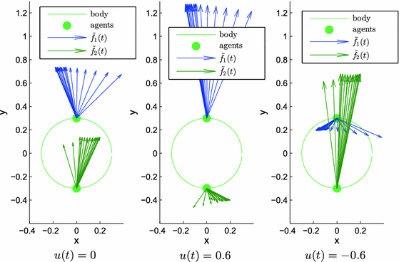
Illustration of the applied forces \(\tilde{f}_1(t), \tilde{f}_2(t)\) in the body-fixed frame in the x-y plane that are in mixed type (\(u(t)=0\)), pull (\(u(t)=0.6\)) and push (\(u(t)=-0.6\)), respectively. The arrows represent the magnitudes and directions of the forces. All the forces (directions and magnitudes) will converge to be constant in the body-fixed frame
-
(2)
when \(u(t)=0.6\), the forces are all pull; and
-
(3)
when \(u(t)=-0.6\), the forces are all push.

Figure 11 shows the effect of the unilateral control \(u(t)\) that makes the forces to be unilateral. As the absolute value \(|u(t)|\) increases, the swing of the directions of the forces \(\tilde{f}_1(t)\) and \(\tilde{f}_2(t)\) will become narrow accordingly (for limited space, the illustration omitted).
For the case of \(n=6\) thrusters, Fig. 12 illustrates the overall applied push forces \(\tilde{f}_k(t), k=1,2,\ldots ,6\), to the rigid body in the body-fixed frame, without the consideration of the friction (\(f_0=M_0=0\), refer to “Appendix B”), \(u(t)=-0.6, t=[5,8]\). Compared with Fig. 11, as the number \(n\) of the thrusters increases from 2 to 6, naturally the magnitudes of the forces decrease, since there are more thrusters that share the same load in the manipulation.

Illustration of the push forces \(\tilde{f}_k(t)\), \(k=1,2,\ldots ,6\), in the body-fixed frame in the \(x\)–\(y\) plane, without friction (\(f_0=M_0=0\)). The arrows represent the magnitudes and directions of the forces. The forces will converge to be constant in the body-fixed frame
Figure 13 illustrates the overall applied push forces \(\tilde{f}_k(t), k=1,2,\ldots ,6\), to the rigid body in the body-fixed frame, with friction (\(f_0=M_0=1\), refer to “Appendix B”), \(u(t)=-0.6, t=[5,8]\), which shows the effect of the friction on the overall applied forces of the thrusters. As compared with Fig. 12, to preserve the same dynamics of the rigid body, the directions of the forces change and the magnitudes of the forces increase significantly to overcome the friction. Certainly, as the values of friction coefficients \(f_0,M_0\) increase, the magnitudes of \(\tilde{f}_k(t), k=1,2,\ldots ,6\) will increase correspondingly (illustration omitted for lack of space).

Illustration of the push forces \(\tilde{f}_k(t)\), \(k=1,2,\ldots ,6\), in the body-fixed frame in the \(x\)–\(y\) plane, with friction \(f_0=M_0=1\). The arrows represent the magnitudes and directions of the forces. The forces will converge to be constant in the body-fixed frame
8 Conclusion
In this paper, we consider the cooperative manipulation of a rigid body by the forces of the attached unilateral thrusters for two cases: (i) the directions of the thrusters are all fixed, and (ii) the directions of the thrusters can swing (i.e., non-fixed directions). For the two cases, we design two decomposition frameworks respectively, on the structure of the applied forces and the control policy such that the linear and angular accelerations of the body are decoupled and controlled independently, and the control that ensures the forces to be unilateral is independent from the linear and angular accelerations (Framework II). As a result, the body is easily controlled, and the design of the control laws in these cases are trivial, as illustrated in the examples of trajectory tracking with friction, and thus, the frameworks will provide convenience on a quick estimation of maximum forces of thrusters needed that is useful in design of physical systems.
The control paradigm in this paper is centralized with global information sharing of the thrusters. The decentralized unilateral control is feasible for manipulation and transportation of the rigid body, but may have difficulties to ensure the requirements that the rigid body is STLC and the controls for rotation/translation dynamics decoupled and linear. If without the assumption of the perfect placement of the thrusters, then manipulation and transportation are of course possible, but probably without the properties expected in Sect. 2.4, provided that no additional compensation added.
There are some questions remain to be investigated, for example, (i) how to design the arrangement of the thrusters and the control laws when some thrusters apply only push forces while others apply only pull forces? (ii) what about when some thrusters have fixed directions while others can have swing directions? (iii) what about when the magnitude of the force of every thruster is limited? (iv) what is even more energy-efficiency solutions for such unilateral manipulations? and (v) the robust analysis without perfect placement of the thrusters, inaccurate measurements, fuel consumption of the thrusters and thus the drifting of the center of mass, possibly with another thruster compensation, needs to be further considered.
When using mobile robots for manipulation instead of attached thrusters, the cooperative manipulation of the rigid body is not a pure manipulation or pure motion coordination problem (such as flocking [23–27], formation [28–31]) of the robots, it requires regulation of both motion (between mobile robots) and interaction forces (between the body and the robots), and this question is challenging and needs to be further investigated; the robustness to individual thruster/robot failure, as well as physical implementations (with communication issues between robots), also needs to be considered in future.
Notes
The mass \(m\) includes the mass of the thrusters; for simplicity, the fuel consumption is not considered.
Refer to Appendix for the controllability of the minimum number of thrusters with \(n=1,2,3\) investigated in [15].
References
Krause, J., Ruxton, G.D.: Living in Groups. Oxford University Press, Oxford (2002)
Krieger, M., Billeter, J., Keller, L.: Ant-like task allocation and recruitment in cooperative robots. Nature 406, 992–995 (2000)
Cretu, A.-M., Payeur, P., Petriu, E.M.: Soft object deformation monitoring and learning for model-based robotic hand manipulation. IEEE Trans. Syst. Man Cybern. B Cybern. 42, 740–753 (2012)
Foresti, G.L., Pellegrino, F.A.: Automatic visual recognition of deformable objects for grasping and manipulation. IEEE Trans. Syst. Man Cybern. C Appl. Rev. 34, 325–333 (2004)
Lionis, G., Kyriakopoulos, K.J.: Centralized motion planning for a group of micro agents manipulating a rigid object. In: Proceedings of the 13th Mediterranean Conference on Control and Automation, pp. 662–667 (2005)
Allais, A.A., McInroy, J.E., OBrien, J.F.: Locally decoupled micromanipulation using an even number of parallel force actuators. IEEE Trans. Robot. 28, 1323–1334 (2012)
Michael, N., Fink, J., Kumar, V.: Cooperative manipulation and transportation with aerial robots. Auton. Robots. 30, 73–86 (2011)
Fink, J., Michael, N., Kim, S., Kumar, V.: Planning and control for cooperative manipulation and transportation with aerial robots. Int. J. Robot. Res. 30, 324–334 (2011)
Feemster, M.G., Esposito, J.M.: Comprehensive framework for tracking control and thrust allocation for a highly overactuated autonomous surface vessel. J. Field Robot. 28, 80–100 (2011)
Rodriguez, A., Mason, M.T., Ferry, S.: From caging to grasping. Int. J. Robot. Res. 31, 886–900 (2012)
Rodriguez, A., Mason, M.T.: Grasp invariance. Int. J. Robot. Res. 31, 236–248 (2012)
Caccavale, F., Muscio, G., Pierri, F.: Grasp force and object impedance control for arm/hand systems. In:16th International Conference on Advanced Robotics (ICAR), pp. 1–6 (2013)
Mesquita, A., Rempel, E.L., Kienitz, K.H.: Bifurcation analysis of attitude control systems with switching-constrained actuators. Nonlinear Dyn. 51, 207–216 (2008)
Pereira, G.A.S., Campos, M.F.M., Kumar, V.: Decentralized algorithms for multi-robot manipulation via caging. Int. J. Robot. Res. 23, 783–795 (2004)
Lynch, K.M.: Controllability of a planar body with unilateral thrusters. IEEE Trans. Autom. Control 44, 1206–1211 (1999)
Lynch, K.M., Mason, M.T.: Dynamic nonprehensile manipulation: controllability, planning, and experiments. Int. J. Robot. Res. 18, 64–92 (1999)
Spong, M.W.: Impact controllability of an air hockey puck. Syst. Control Lett. 42, 333–345 (2001)
Partridge, C.B., Spong, M.W.: Control of planar rigid body sliding with impacts and friction. Int. J. Robot. Res. 19, 336–348 (2000)
Forni, F., Teel, A.R., Zaccarian, L.: Follow the bouncing ball: global results on tracking and state estimation with impacts. IEEE Trans. Autom. Control 58, 1470–1485 (2013)
Esposito, J.M.: Decentralized cooperative manipulation with a swarm of mobile robots. In: Proceedings of the IEEE/RSJ International Conference on Intelligence Robots Systems, pp. 5333–5338 (2009)
Esposito, J.M.: Decentralized cooperative manipulation with a swarm of mobile robots: the approach problem. In: Proceedings of the American Control Conference, pp. 4762–4767 (2010)
Li, W., Spong, M.W.: Unified cooperative control of multiple agents on a sphere for different spherical patterns. IEEE Trans. Autom. Control 59, 1283–1289 (2014)
Dong, W.: Flocking of multiple mobile robots based on backstepping. IEEE Trans. Syst. Man Cybern. B Cybern. 41, 414–424 (2011)
Li, W., Spong, M.W.: Stability of general coupled inertial agents. IEEE Trans. Autom. Control 55, 1411–1416 (2010)
Li, W., Spong, M.W.: Analysis of flocking of cooperative multiple inertial agents via a geometric decomposition technique. IEEE Trans. Syst. Man Cybern. Syst. doi:10.1109/TSMC.2014.2318013
Zavlanos, M.M., Tanner, H.G., Jadbabaie, A., Pappas, G.J.: Hybrid control for connectivity preserving flocking. IEEE Trans. Autom. Control 54, 2869–2875 (2009)
Moshtagh, N., Jadbabaie, A.: Distributed geodesic control laws for flocking of nonholonomic agents. IEEE Trans. Autom. Control 52, 681–686 (2007)
Zavlanos, M.M., Egerstedt, M.B., Pappas, G.J.: Graph-theoretic connectivity control of mobile robot networks. Proc. IEEE. 99, 1525–1540 (2011)
Kan, Z., Dani, A.P., Shea, J.M., Dixon, W.E.: Network connectivity preserving formation stabilization and obstacle avoidance via a decentralized controller. IEEE Trans. Autom. Control. 57, 1827–1832 (2012)
Mas, I., Kitts, C.: Obstacle avoidance policies for cluster space control of nonholonomic multirobot systems. IEEE/ASME Trans. Mechatron. 17, 1068–1079 (2012)
Kitts, C.A., Mas, I.: Cluster space specification and control of mobile multirobot systems. IEEE/ASME Trans. Mechatron. 14, 207–218 (2009)
Author information
Authors and Affiliations
Corresponding author
Appendices
Appendices
1.1 Appendix A
Lynch [15] investigated the controllability of the rigid body with the unilateral thrusters. Define the state of the rigid body as \((q,\dot{q})\), where the configuration \(q\) is the state of \(x(t)\) and \(\psi (t)\). Define \(R^V(q_0,\dot{q}_0,T)\) to be the reachable set from \((q_0,\dot{q}_0)\) at time \(T>0\) by feasible trajectories remaining in the neighborhood \(V\) of \((q_0,\dot{q}_0)\) at times \(t\in [0,T]\). Define \(R^V(q_0,\dot{q}_0,\le T)=\bigcup _{0\le t \le T}R^V(q_0,\dot{q}_0,t)\). The body is STLC from \((q_0,\dot{q}_0)\) if \(R^V(q_0,\dot{q}_0,\le T)\) contains a neighborhood of \((q_0,\dot{q}_0)\) for any neighborhood \(V\) and all \(T>0\). The body is controllable from \((q_0,\dot{q}_0)\) if, for any \((q_1,\dot{q}_1)\in TC\), there exists a finite time \(T\) such that \((q_1,\dot{q}_1)\in R^{TC}(q_0,\dot{q}_0,T)\).
The controllability of the rigid body with the unilateral thrusters [15] it that: (1) The body is controllable with two thrusters if and only if they provide torque of opposite signs; (2) the body is STLC on the zero velocity section \((q,\mathbf {0})\) with three thrusters if their lines of action intersect at a single point which is not the center of mass, and the thrusters positively span the plane.
The controllability of the body with the arbitrary forces of the attached agents is implied in [15]: It is controllable with one or more agents and is not STLC with only one agent.
1.2 Appendix B: Consideration of external forces
If the external forces on the body are included, while the dynamics of the body requires to satisfy the concerns (Sect. 2.4), then these external forces are assumed to be precisely known for the controllers and the controllers just introduce some term to cancel them. The external force (e.g., friction) under such framework can be easily incorporated into the dynamics of the body, that is, we divide the control policy into two parts: One is the pure control for the dynamics of the body without considering the external force, and the other is designed to cancel or overcome the external force, thus making the design of the dynamics trivial and separated from consideration of the external force. Consider the dynamics:
where \(f_e(t)\in \mathbb {R}^2\) and \(M_e(t)\in \mathbb {R}\) are the external force and moment, respectively.
Consider the external force \(f_e(t)\) and moment \(M_e(t)\) as the friction on the body. Assume the friction on the body is always exerted in a direction that opposes movement for kinetic friction (with the constant magnitude) or potential movement for static friction (with the magnitude as the function of the net applied force), and for simplicity and without loss of generality, assume the same coefficient for static and kinematic frictions, i.e.,
where \(f_0, M_0>0\) are the maximum magnitudes of the friction force \(f_e(t)\) and moment \(M_e(t)\), respectively, and for convenience, denote
as the overall forces of moments of the thrusters, respectively. The sign function \(\hbox {sgn}(y)\) of a real parameter \(y\) is defined as follows:
The friction has the properties: (1) \(f_e(t)\) always has the opposite direction of the force \(f(t)\) or \(\dot{x}(t)\); (2) \(M_e(t)\) always has the opposite sign of \(M(t)\) or \(\dot{\psi }(t)\).
From the above analysis, the dynamic (1)–(2) reduce to
To simplify the design of the control laws, we consider the control inputs \(g(t)\) and \(a(t)\) with two parts:
where \(g^*(t)\in \mathbb {R}^2\) and \(a^*(t)\in \mathbb {R}\) are the pure controls for the dynamics of the body without considering the external force, and \(g_e(t)\in \mathbb {R}^2\) and \(a_e(t)\in \mathbb {R}\) are the terms to cancel or overcome the external force:
thus making the design of dynamics of the body separated from the consideration of external force. The control policy is illustrated in Fig. 14. In this case,
and, hence, the control of translation and the control of rotation of the body are completely decoupled and linear, and independent from the unilateral control \(u(t)\). Therefore, the body is STLC and can be easily controlled by suitable choice of \(g^*(t), a^*(t)\) and thus \(g(t), a(t)\) as control inputs in the inertial frame. As a result, the control of the rigid body becomes trivial.

The design diagram of the control policy
Consider friction defined in (34) and (35), design:
where \(m_0:= \frac{m}{\sum _{k=1}^N 1/\ell _k}\), \(I_0:=\frac{I}{\sin (\theta _0)\sum _{k=1}^N \ell _k}\), and \(\frac{g^*(t)}{||g^*(t)||}|_{g^*(0)=\mathbf {0}} := \mathbf {0}\).
Proposition A1
For the friction defined in (34) and (35) and \(g_e(t)\), \(a_e(t)\) defined in (44) and (45), the result (42)–(46) holds.
Proof
From (22) and the structure of forces, we have
For \(\dot{x}(t)=\mathbf {0}\), from (40) and (44), we have:
-
(i)
when \(g^*(t)= \mathbf {0}\), then \(g(t)= \mathbf {0}, f(t)= \mathbf {0}\), thus \(f_e(t)= \mathbf {0}\);
-
(ii)
when \(g^*(t)\ne \mathbf {0}\), then \(||g(t)||\ge \frac{m_0}{m}f_0\), i.e., \(||f(t)||\ge f_0\), and \(f_e(t)\) in (38) is:
$$\begin{aligned} f_e(t) = -f_0 f(t)/||f(t)|| = -f_0 g(t)/||g(t)|| \end{aligned}$$from (40), (44), \(g(t) +\frac{m_0}{m}f_e(t) = g^*(t)+\frac{m_0}{m}f_0 \frac{g^*(t)}{||g^*(t)||} - \frac{m_0}{m}f_0\frac{g(t)}{||g(t)||} = g^*(t)\).
For \(\dot{x}(t)\ne \mathbf {0}, g_e(t)\) cancels \(f_e(t)\) directly. Then Eq. (38) reduces to Eq. (30).
Similarly, we have the dynamics of \(\ddot{\psi }(t)\).\(\square \)
Remark 11
When the friction is not considered, i.e., \(f_0=M_0=0\), then \(g(t)=g^*(t), a(t)=a^*(t)\).
For the trajectory tracking in Sect. 7.1, simply let
then \(x(t)\rightarrow x_d(t), \dot{x}(t)\rightarrow \dot{x}_d(t)\), and \(\psi (t)\rightarrow \psi _d(t), \dot{\psi }(t)\rightarrow \dot{\psi }_d(t)\).
Rights and permissions
Open Access This article is licensed under a Creative Commons Attribution 4.0 International License, which permits use, sharing, adaptation, distribution and reproduction in any medium or format, as long as you give appropriate credit to the original author(s) and the source, provide a link to the Creative Commons licence, and indicate if changes were made.
The images or other third party material in this article are included in the article’s Creative Commons licence, unless indicated otherwise in a credit line to the material. If material is not included in the article’s Creative Commons licence and your intended use is not permitted by statutory regulation or exceeds the permitted use, you will need to obtain permission directly from the copyright holder.
To view a copy of this licence, visit https://creativecommons.org/licenses/by/4.0/.
About this article

Cite this article
Li, W., Spong, M.W. Decomposition frameworks for cooperative manipulation of a planar rigid body with multiple unilateral thrusters. Nonlinear Dyn 79, 31–46 (2015). https://doi.org/10.1007/s11071-014-1643-3
Received:
Accepted:
Published:
Issue Date:
DOI: https://doi.org/10.1007/s11071-014-1643-3