A complete methodology to assess hydraulic risk in small ungauged catchments based on HEC-RAS 2D Rain-On-Grid simulations

Abstract

This paper explores the use of the rain-on-grid (or direct rainfall) method for flood risk assessment at a basin scale. The method is particularly useful for rural catchments with small vertical variations and complex interactions with man-made obstacles and structures, which may be oversimplified by traditional hydrologically based estimations. The use of a hydrodynamic model solving mass and momentum conservation equations allows the simulation of runoff over the watershed at a basin scale. As a drawback, more detailed and spatially distributed data are needed, and the computational time is extended. On the other hand, a smaller number of parameters is needed compared to a hydrological model. Roughness and rainfall loss coefficients need to be calibrated only. The direct rainfall methodology was here implemented within the two-dimensional HEC-RAS model for the low-land rural, and ungauged, watershed of the Terdoppio River, Northern Italy. The resulting hydrographs at the closing section of the watershed were compared to synthetic design hydrographs evaluated through pure hydrological modelling, showing agreement on the peak discharge values for the low-probability scenarios, but not on the total volumes. The results in terms of water depth and flow velocity maps were used to create flood hazard maps using the Australian Institute for Disaster Resilience methodology. The Index of Proportional Risk model was then adopted to generate a basin-scale flood risk map, by combining flood hazard maps, damage functions for different building-use classes, and the value of reconstruction and content per unit area.

1 Introduction

The frequency and unpredictability of floods have been on the rise in recent years, largely due to human interventions to the natural environment and the effects of global climate change (Arnell and Gosling 2016). Urbanization within river flood plains has also increased the exposure of communities to flood hazards. Developing countries, with their high levels of susceptibility due to poor socio-economic conditions and unplanned settlements, are disproportionately affected by these disasters. On the other hand, developed countries, with their infrastructures, face significant economic losses if floods are not effectively managed (Brody et al. 2007).

The European Union has taken a particular interest in pluvial floods, which are triggered by intense short-duration rainfalls, encouraging studies and simulations of these events, which may cause damages to the whole basin and not only to the areas near the main channel (Hu et al. 2023). In this frame, 2D rain-on-grid (ROG) approaches can be particularly beneficial. The ROG approach, or direct rainfall method as defined in Hall (2015), entails the application of net rainfall to individual cells within a two-dimensional (2D) domain. The subsequent runoff is then reproduced using a 2D hydrodynamic model. This method has gathered increasing interest among flood modelers due to its simplicity and flexibility (Barbero et al. 2022). Another relevant benefit of direct rainfall methods is that the hydrological response of the watershed to the input rainfall is physically simulated and not synthetically interpreted, as in traditional hydrological methods.

Among existing studies employing the ROG method, Hall (2015) employed the MIKE21 model developed by the Danish Hydraulic Institute (DHI) to perform an application for different return periods on a 20 m resolution grid with the objective of exploring the pros and cons of the ROG method in design flood simulations and floodplain mapping. Cea and Bladé (2015) developed a method known as Decoupled Hydrological Discretization (DHD) to solve the 2D Shallow Water Equations (SWE) in hydrodynamic ROG applications, and the ROG approach was also integrated and tested in the 2D hydrodynamic model TELEMAC-2D (Broich et al. 2019). Caviedes-Voullième et al. (2023) developed a high-performance parallel-computing shallow-water solver called SERGHEI (SERGHEI-SWE). This code adopts a finite-volume method and a second-order explicit time-stepping scheme to solve the hydrodynamics of overland flow across various scales from hillslope to catchment levels. Aureli et al. (2020) developed a GPU-based parallel numerical model for the solution of the 2D SWE called PARFLOOD Rain for the simulation of rainfall-runoff processes in a watershed. The model is characterized by a finite-volume explicit discretization technique, which is well-balanced and s second-order accurate. Thanks to the structure of the algorithm, the scheme is also numerically stable for overland flow.

In the context of ROG simulations, the Hydrologic Engineering Center-River Analysis System (HEC-RAS) code developed by the US Army Corps of Engineers has been extensively used to solve the SWE and simulate hydrodynamic-based surface runoff at a catchment-scale. The hydrodynamic code of HEC-RAS 2D has been extensively validated. For example, Costabile et al. (2020, 2021) performed a benchmark study of HEC-RAS 2D for simulating ROG scenarios, comparing the results of this model against analytical solutions, experimental data, and numerical solutions resulting from an in-house code. The results revealed that the “full momentum” solver of HEC-RAS 2D provided similar results to the state-of-the-art in-house model in terms of flood-wave shape, peak discharge, and time to peak. Instead, the simpler yet faster “diffusive wave” (DSW) solver of HEC-RAS 2D tends to overestimate the peak discharge values and simulate faster flood waves. Hariri et al. (2022) developed a methodology for domain decomposition to model very large catchments through direct rainfall with HEC-RAS 2D, to avoid simulation failure due to memory shortage when the discretization yields too large linear systems. David and Schmalz (2021) performed a comprehensive investigation into the behavior of the HEC-RAS 2D model, with a particular emphasis on examining the impact of spatial resolution on the results of ROG simulations in a small ungauged low-land study area, their analysis showed that for coarser grids, the runoff is delayed at the catchment outlet due to low water layer that is computationally kept in the cells. Zeiger and Hubbart (2021) proposed an integrated modelling approach that employed a coupled-modelling routine. This involved the use of two specific tools, namely the Soil and Water Assessment Tool (SWAT), a hydrological watershed model that determined net rainfall rates, and HEC-RAS 2D, which was used for ROG simulations. Krvavica and Rubinić (2020) fed HEC-RAS 2D with direct precipitation to analyze a small ungauged catchment. The primary goal of their research was to evaluate the impact of various storm hyetographs and rainfall durations on the outflow from the catchment.

Net rainfall estimation is a crucial step for proper ROG modelling, since the uncertainty and the correct choice of input data can dramatically affect the performance of physically based rainfall-runoff models (Fraga et al. 2019). In addition to this, the generation of the computational mesh also plays a key role in the application of the ROG methodology, a proper grid design being a trade-off between accuracy and computational cost. In David and Schmalz (2020), a high discrepancy between the ROG model outflow and inflow was found for a coarse mesh set-up, while for a fine mesh set-up the effect was less pronounced. This problem may indicate a limitation of the method in representing flows at very shallow depths.

The resolution of the Digital Terrain Model (DTM) should be critically selected as well. According to Habtezion et al. (2016), there is a trade-off between the resolution and the overall computational efficiency, as using a high-resolution DTM can provide more accurate results, but the increased data volume and processing time can be prohibitively time-consuming. Therefore, it is important to determine the optimal resolution that balances accuracy and computational feasibility. In that study, resolutions up to 10 m provided comparable simulation results for general basin-scale simulations. In addition, the ROG approach may require a modification of the DTM to appropriately represent the required drainage network. This process can be both time consuming and subjective. Moreover, the computational time required by the model is potentially increased if compared to traditional techniques, which can make the simulation of multiple events challenging (Hall 2015). Johnson (2013) performed a comparison of direct rainfall and lumped-conceptual rainfall-runoff routing methods, revealing that direct-rainfall models showed reduced and attenuated runoff due to storage effects (Johnson 2013). A further parameter that needs to be critically evaluated when using a ROG model is the roughness coefficient (Caddis et al., 2008; Johnson 2013). According to David and Schmalz (2020), the value of the Manning coefficient should be increased to fit the requirements of overland flow. Moreover, shallow overland flows may be outside of the typical range where Manning’s flow resistance equation is applicable, or outside of the solution scheme of the model (Hall 2015).

The ROG capabilities of HEC-RAS 2D are here in employed to produce flood hazard maps for a rural ungauged catchment, to assess hydraulic risk through an integrated hydrodynamic approach commonly employed to model urban flood risk. From flood hazard maps, basin-scale flood-risk maps are then elaborated through the Index of Proportional Risk (IRP) model. As literature definitions of risk (Intergovernmental Panel on Climate Change 2012; Mourelatou 2020; The Federal Emergency Management Agency 2023; Nations Office for Disaster Risk Reduction 2015) state, the assessment of flood risk must consider both the probability of a flood event and the related potential consequences, superimposing Hazard, Exposure and Vulnerability components (Lavell et al. 2012) for the selected area. To this aim, building exposure and vulnerability in the study area are also estimated. For validation purposes, the flood hydrographs at the basin closing section, obtained from ROG modelling, were compared to Synthetic Design Hydrographs obtained through ordinary hydrological techniques. The main aim of this study is to propose an integrated hydrodynamic approach based on a free-to-use model of widespread use and data such as geological and land registry maps of common availability in most countries, easing its implementation. By using publicly available data, we can enhance the accuracy of our modelling and risk analysis without running into significant costs associated with data acquisition. This approach also promotes transparency and allows other researchers to replicate and develop our methodology. The proposed approach can be applied using as hazard maps the results of any ROG model.

2 Materials and methods

Figure 1 provides an overview of the proposed procedure for the assessment of flood risk, which has been applied to a small rural watershed selected as a case study. When first selecting the study area and retrieving the needed data, the focus was to ensure a balance between the accuracy of the data sources and their costs, trying mainly to use open data. The following step was analyzing the data by preparing the net rainfall time series and estimating the Manning’s coefficients according to land use. The third step was the set-up of the rain-on-grid model in HEC-RAS, i.e., generating the computational grid, preparing the boundary conditions, and finally applying the net rainfall as an input for each considered return period T. The results of the 2D ROG model were last used to estimate the flood hazard and flood risk for the buildings in the study area.

Fig. 1

Overview of the procedure for the hydraulic modelling and risk evaluation

2.1 Study area

The case study considered here is the upstream watershed of the Terdoppio Novarese River in the Piedmont region, North-Western Italy (Fig. 2a). The study area originates from the river springs in the hills of the Novara province and extends up to the bridge of the Novara-Arona railway upstream of the Novara urban center, where the closing section is placed (Fig. 2b). This closing section also marks the upstream limit of the Area of Potential Significant Flood Risk (APSFR) designated by the Po River Basin District Authority (Autorità di Bacino Distrettuale del fiume Po, AdBPo) within its Flood Risk Management Plan (“Piano di Gestione Rischio Alluvioni”—PGRA), based on the EU Floods Directive 2007/60/EC. The main morphological properties of the studied catchment are given in Table 1.

Fig. 2

Study area of the Terdoppio Novarese basin in North-Western Italy (a) and b DTM of the considered watershed

Table 1 Main morphological features of the considered Terdoppio Novarese basin.

2.2 Data acquisition

The datasets required to implement the described methodology are:

• Land Use: the CORINE Land Cover (CLC) 2018 raster with 100 m resolution describing the land use status of the year 2018 (Fig. 3) was downloaded from the Copernicus Land Monitoring Service website (Copernicus Services 2018a).

  Fig. 3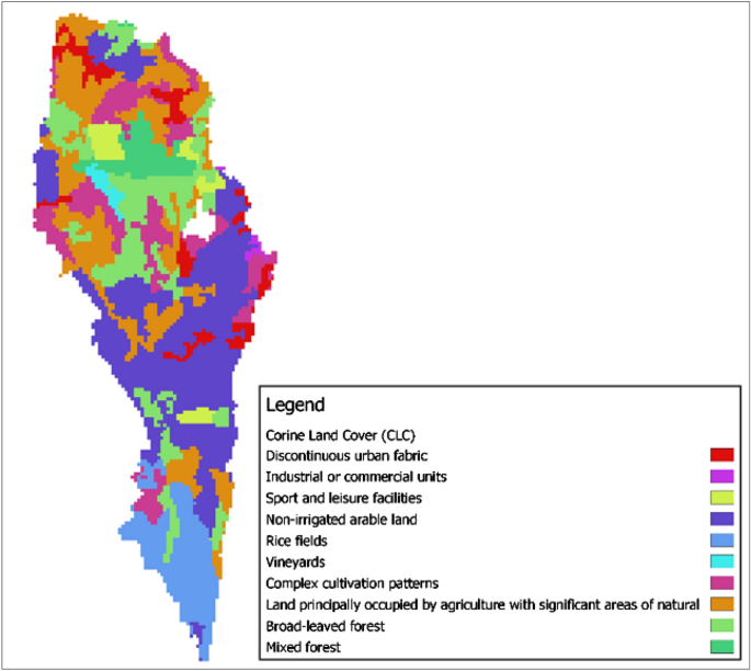

  

  CORINE Land Cover 2018 map of the considered Terdoppio Novarese basin

• Digital Terrain Model (DTM): a 5 m DTM was downloaded from the geographical portal of the Piedmont Region and pre-processed using GIS tools to get a depression-free DTM ready for use.

  Fig. 4

  

  Drainage condition (a) and soil type (b) maps of the considered Terdoppio Noverese basin

• Soil Cover and Drainage Conditions Maps: the soil type and drainage condition maps (Fig. 4), relevant for the evaluation of net rainfalls, were downloaded from the geographical portal of the Piedmont Region (Piemonte region 2020).

• Imperviousness Percentage Map: a raster layer capturing the soil impervious fraction (Fig. 5) was downloaded from the Copernicus Land Monitoring Service (Copernicus Services 2018b).

  Fig. 5

  

  Impervious percentage map of the considered Terdoppio Novarese basin

• Intensity-Duration-Frequency (IDF) Rainfall Curves: The IDF rainfall curves at the centroid of the considered Terdoppio Novarese basin for the selected return periods were obtained from the Piedmont Regional Environmental Protection Agency Intense Rainfall Atlas webapp (ARPA Piemonte 2013).

  The webapp allows retrieving the gross rainfall depths for the selected return periods and event durations ranging from 10 min to 24 h at any location within the Piedmont Region. The regional statistical analysis leading to this dataset employed all available rainfall data from 1913 onwards and made use of the Generalized Extreme Value (GEV) probability distribution. The resulting intensity-duration curve used in this study is:

  $$h = K_{T} 32.375t^{0.314}$$

  (1)

  where h is the gross rainfall depth in mm, t is the rainfall duration in hours and K_T is a given growth factor function of the return period (Table 2), obtained through the regional analysis. Six return periods were considered in this study: 10, 20, 50, 100, 200, 500 years.

  Table 2 Growth factor values for the considered return periods from the Intense Rainfall Atlas for the centroid of the studied watershed.

• Manning’s Coefficients: the CORINE Land Cover 2018 map (Copernicus Services 2018a) and standard Manning’s roughness coefficient tables (Chow 1959) were used to determine the values of the roughness coefficients in this study (Fig. 6). For the main channel, a single value n = 0.035 ms^−1/3 was employed.

  Fig. 6

  

  Raster of Manning’s coefficients (in m s^−1/3) based on the CORINE Land Cover map

• Exposed Elements: for this case study, the receptors are all the buildings inside the Terdoppio Novarese basin. The building dataset is available from the Geoportale Regione Piemonte, as part of the BDTRE GIS database. Figure 7 shows a portion of the buildings of the municipality of Mezzomerico, located at the center of the basin. This GIS layer provides for each building the surface area and the mean height, generally obtained through aero photogrammetry. Superelevated buildings (on a porch) are indicated. Most importantly, information on the use of each building is provided, categorizing them into three classes, i.e., Residential buildings, Commercial buildings, and Industrial buildings.

  Fig. 7

  

  Buildings inside the municipality of Mezzomerico, categorized according to the three use classes

• Exposure Value: the ADE (Agenzia delle Entrate/Income Revenue Authority) website “Observatory of the Housing Market” (OMI) (Agenzia Entrate) provides public data on the economic values of residential, commercial, and industrial categories of receptors, expressed per unit area. Zones deemed to be economically homogenous have been created inside each Italian municipality. Subcategories have been established for each zone and each building class, with minimum and maximum economic values. The OMI dataset represents only the property values and disregards the value of their contents. Wide value fluctuations are present across the watershed, even inside homogenous OMI zones. In the present study the mean values of all the OMI zones for every building class will be employed, to enable a uniform evaluation across the whole watershed (Table 3).

  Table 3 Assumed mean value per unit area of building structures based on the OMI database and of contents based on the JRC technical report (Huizinga et al. 2017) for the considered building classes.

  The content value for each building class was taken from the JRC (Joint Research Center) technical report by Huizinga et al. (2017), which reports flood-damage functions for EU member states based on collected damage values (Table 3).

• Vulnerability functions: in this work, we focused only on the vulnerability of buildings, which refers to the susceptibility of buildings to be damaged or destroyed by floods. Building vulnerability can vary significantly between different regions and communities due to the heterogeneous design, construction materials, and height above flood level, so that a one-size-fits-all approach to assessing building vulnerability is not appropriate. Since there are no established vulnerability curves for the Italian context, significant uncertainties exist on vulnerability quantification. For this case study, it was decided to employ the vulnerability curves for the whole European context given by the JRC (Huizinga et al. 2017), according to which the vulnerability of an exposed element ${VR}_{i}$ is a function of the maximum water depth, inside the area occupied by each receptor h_i,max.

  $$VR_{i} = VR_{i} \left( {h_{i,max} } \right)$$

  (2)

  The vulnerability functions are provided by the JRC (Huizinga et al. 2017), according to the use of the considered receptors (buildings). Figure 8 shows as an example the employed damage factor curve in function of water depth for residential buildings. The damage function was interpolated to provide continuous values to estimates damage values for a range of inputs based on discrete data points.

  Fig. 8

  

  Damage function from the JRC technical report (Huizinga et al. 2017) for residential buildings

2.3 Data analysis

The evaluation of net rainfall was carried out according to the steps described in Fig. 9, by means of the SCS-CN method (United States Department of Agriculture 1985) and making use of the HEC-HMS v4.9 hydrological model.

Fig. 9

Methodology for the evaluation of net rainfalls

The first step consisted in the choice of the shape of the gross hyetograph. A Chicago synthetic storm hyetograph (Keifer Client and Hsien1957) was adopted, built employing the IDF curve (ARPA Piemonte 2013) taking into account a time of concentration of 10 h, obtained according to the Giandotti formula. The Hydrological Soil Groups (HSG) for the application of the SCS-CN method were then determined. Based on the analysis of both the soil cover and drainage condition maps of the catchment (Fig. 4), the study area consists of only two HSGs, namely the A and B groups (Fig. 10). Curve Numbers (CNs) were then defined integrating the CORINE Land Cover (Copernicus Services 2018a) and HSG datasets. Table 4 presents the values of the CN reference values (Řehánek et al. 2019) for the land use categories present in the study area for each HSG under Antecedent Moisture Condition II (AMC II).

Fig. 10

Hydrological soil groups (HSGs) map of the considered Terdoppio Novarese basin

Table 4 Curve Number values for each land use type and hydrological soil group (HSG) present in the Terdoppio Novarese basin for AMC II, based on (Řehánek et al. (2019)

Figure 11 shows the final CN map resulting from the combination of the land cover and HSG maps. A single spatial-average value CN_avg = 71 was determined for the watershed and used for the rainfall-runoff transformation. Initial hydrological losses equal to 20% of the maximum infiltration losses were assumed, as per the standard SCS-CN method. Finally, net Chicago hyetographs were produced through HEC-HMS for the considered return periods. Figure 12 shows the resulting net hyetographs for the return periods of 500 and 10 years.

Fig. 11

SCS Curve Number raster of the considered Terdoppio Novarese basin

Fig. 12

Net hyetographs resulting from the HEC-HMS calculation of the gross and net Chicago hyetographs on the study area for a return period of 10 years (a) and 500 years (b)

2.4 2D ROG modelling

The HEC-RAS v6.2 two-dimensional (2D) code solves on a Finite Volume (FV) discretization either the simplified 2D Diffusion Wave Equations (DWE) or the complete Shallow Water Equations (SWE), the latter using either a Eulerian–Lagrangian technique for advection (SWE-ELM) or a Eulerian approach for advection (SWE-EM) (US Army Corps of Engineers). This last option was chosen for the present study. (US Army Corps of Engineers). The solution is performed on an unstructured grid with a constant spatial resolution of 15 m, created from the 5 m-resolution DTM (Geoportale Piemonte region) using the RAS Mapper meshing module of HEC-RAS. The final mesh consists of over 331 000 cells, each having 3 to 8 cell faces. The main grid remains connected to a sub-grid directly reflecting the high-resolution Digital Terrain Model. This feature allows computing the hydraulic variables such as wetted area and perimeter on a higher resolution mesh than the computational one, thus leading to better-quality results without compromising computational times. Each computational cell must then be pre-processed to calculate the additional information for the sub-grid technique.

No upstream boundary condition on water discharge was employed, the model being fed with the net rainfall series calculated with HEC-HMS for each return period (Fig. 12). Dry-bed conditions were assumed, due to the negligible base flow of the Terdoppio River and its inflows, compared to the entity of the reproduced flood events. The downstream boundary condition was set to normal depth with a bottom slope S = 0.001, close to the actual local value. The uniform flow approximation is legitimated by the negligible influence of the downstream boundary condition on the downstream simulated discharge hydrographs.

The simulations lasted approximately 6 h on an AMD Ryzen 9 3950x (16 cores, 32 threads) workstation with 64 GB of RAM.

2.5 Flood hazard and flood risk estimation

Techniques for flood hazard estimation are divided into two main categories:

• (i) Methods based on flood intensity (i.e., on either flow depth or a combination of flow depth and velocity) and probability—as adopted for instance by U.S. Army Corps of Engineers (1995), Po River Basin Authority (1999) and Regione Sicilia (2004).

• (ii) Methods based on flood intensity only, as indicated by the guidelines issued by U.S departement Department of interior Interior bureau Bureau of reclamation Reclamation (1988), MATE-METL (1999) and (Italian Higher Institute for Environmental Protection and Research ISPRA 2012).

In this work, we adopted a method belonging to the second category, the Australian Institute for Disaster Resilience (AIDR) hazard classification, which combines water depth h and velocity V information to estimate flood hazard (AIDR 2017). Six hazard classes are defined (Table 5).

Table 5 AIDR hazard classification (AIDR 2017).

The Index of Proportional Risk (IRP) method (Franzi et al. 2018) was employed for risk assessment and quantification in this study. The IRP model has been successfully used in various case studies within Piedmont (Franzi et al. 2016, 2018) demonstrating its effectiveness in estimating flood risk for the present context. The IRP model calculates an “index” that is based on a scientific approach to risk and damage estimation, considering available regional and national databases. This approach considers factors such as the flood characteristics, vulnerability of the region, and the value of the assets at risk, providing a reliable and comprehensive estimate of flood risks and damages in the Piedmonte Region. Despite the challenges in IRP calibration, it is considered a valuable method for estimating the overall damage resulting from a flood. However, it is important to note that the actual total damage caused by floods can be much higher than the damage to residential or commercial properties only that is calculated through the IRP.To calculate the IRP, the following expression is applied:

$$IRP_{i} = \frac{1}{T}\mathop \sum \limits_{i}^{N} e_{i} \cdot A_{i} \cdot VR\left( h \right)_{i}$$

(3)

where i is the generic receptor in the considered area, N is the total number of receptors, T is the return period in years, A is the area of the receptor in m², e is the receptor value in €/m², and VR(h_max) is the estimated vulnerability, as function of the maximum water level h. The IRP is given in €/year, and it refers to the Expected Annual Damage (EAD), i.e., the yearly expenses that occur if monetary damages arising from all hazard probabilities and magnitudes were equally distributed over time. It represents the yearly average expense related to natural hazard (Colorado water Water conservation Conservation board Board 2020).

The hazard aspect of flood risk is related to the results of 2D hydraulic modelling, primarily water depth and velocity maps. Regarding exposed elements, for this case study, all the buildings within the extent of the studied watershed were considered, as given by the employed GIS dataset (Geoportale Piemonte region). As regards vulnerability, a water depth value was assigned to each building for each return period considering the mean value over all the cells included in the building footprint. Finally, following the calculation of the EAD, the receptors were divided into four risk classes (R1, R2, R3, R4) according to Table 6.

Table 6 Considered risk classes.

3 Results and discussion

3.1 Discharge hydrographs at the basin outlet

The discharge hydrographs at the outlet section resulting from the 2D ROG model of the Terdoppio case study for the considered return periods are shown in Fig. 13. The peak discharges are also reported in Table 7. The time to peak was found to be inversely correlated to the return period (Table 7), with a longer lag time observed for higher probability events, as found by Barbero et al. (2022b).

Fig. 13

Hydrographs resulting from the ROG simulations for each return period at the outlet section of the basin

Table 7 Peak discharge and time to peak for each considered return period.

3.2 Comparison between ROG model hydrographs and synthetic design hydrographs

The hydrographs obtained through ROG modeling at the closing section of the considered watershed were compared with Synthetic Design Hydrographs (SDH) resulting from a purely hydrological analysis. These SDHs were obtained from water level observations at the ARPA Piemonte gauging station of Caltignaga, located 1.9 km upstream of the considered closing section. Due to the small distance, negligible variations in the flow rate are expected between the two sections. This station was activated in 2003 and the related stage-discharge relationship was calibrated thanks to a collaboration between ARPA Piemonte and the University of Pavia inside the PGRA. The SDHs were then developed from the resulting discharge data by the University of Parma and the Polytechnic University of Turin as part of the PGRA. Specifically, peak discharges were determined through the ARPIEM method (Laio et al. 2011), while the shape of the hydrographs was defined according to the method proposed by (Tomirotti and Mignosa (2017).

Results show that the peak discharges estimated by the ARPIEM method are in general greater than those resulting from the HEC-RAS 2D ROG model (Table 8), with a decreasing difference for increasing return periods. For the highest return period T = 500 years, the situation reverses, with a 3% larger peak discharge obtained by the ROG model. These discrepancies might be attributed to the hydrological assumptions and uncertainties associated with both methods. Note that, in any case, statistical hydrology was nevertheless used to determine the rainfall input of the ROG model. Furthermore, the discharges obtained by the ROG methodology may be considered as the maximum discharges that can physically reach the outlet section for a given rainfall input, considering the morphology of the watershed, whereas the purely hydrological method returns peak discharges dependent on probabilistic extrapolations only. Therefore, ROG simulations can potentially lead to more accurate and physically based peak discharges for hazard evaluation, depending only on the representativeness of the net rainfall input.

Table 8 Comparison between the peak discharges of the SDHs generated in the context of the PGRA and those obtained with the present ROG modelling.

Both SDH and ROG methods have strengths and weaknesses. SDHs are simple and easy to use, making them suitable for small-scale studies and quick estimates. On the other hand, hydrographs resulting from ROG models require more data and computational power, but they lead to a more accurate representation of the catchment response to rainfall, as the method can consider the spatial distribution of rainfall and the heterogeneity of the catchment.

3.3 Flood depth and velocity mapping

One of the most important HEC-RAS outputs in the context of ROG modelling at basin scale are flooding maps. However, it is usually necessary to define a water depth threshold for the identification of the flooded cells for a more solid visualization of the results. Flood extents and water depths simulated by the HEC-RAS model were here extracted for the considered flood events. Figures 14 and 15 display sample results for the 500- and 10-year return periods, respectively. The overall flooded areas share the same pattern and are very close, except for the downstream part of the basin, where a major difference in the flooded extent can be observed. For this case study, the velocity maps show an identical behavior under all return periods. High velocities are present only inside the main channel, whereas velocities drop down to zero near the boundaries of the flooded area.

Fig. 14

Maximum water depth map for the return period T = 500 years

Fig. 15

Maximum water depth map for the return period T = 10 years

3.4 Flood hazard classification

The water depth and velocity fields simulated in HEC-RAS were used for flood hazard mapping, which was performed with the AIDR methodology through the RASter Calculator module of HEC-RAS. The resulting map for the return period of 500 years is reported in Fig. 16. Over 75% of the existing buildings within the watershed are within the H1 class, nearly 23% fall in classes H2 and H3, less than 2% in class H4, only 0.4% in class H5 and 0% in class H6. The last 2 hazard classes are almost confined to the main channel of Terdoppio, so that only structures on the banks lie inside such classes. According to the AIDR classification (Table 5), buildings located in class H1 are not exposed to structural risk and are generally safe. For the H2 and H3 zones, mobility is at significant risk for people and vehicles, yet buildings are still safe. The hazard maps for smaller return periods display the same behavior with minor differences in class partition percentages among buildings. No areas within the H6 class are present for the return periods of 20 and 10 years, even inside the Terdoppio main channel.

Fig. 16

AIDR Hazard map for the return period T = 500 years

3.5 Flood risk assessment

Following the IRP calculation procedure, the Expected Annual Damage (EAD) for every building (receptor) range from zero (for buildings not affected by flooding) to more than 200,000 €/y. The total expected annual damage for all buildings within the study area is found to be a little over 10,000,000 €/y. The total annual damage for each building class (sum of the EAD values for each building) is reported in Table 9.

Table 9 Total EAD for buildings of each building class for the considered Terdoppio Novarese watershed.

The results of the IRP calculation reveal significant variations in EAD, depending on the building class and the employed vulnerability function. Other important factors that affect the IRP values are the height and surface area of the buildings. Figure 17 shows a sample IRP risk map for the town of Divignano, located in the upstream right portion of the watershed. The accuracy and reliability of flood risk assessment are heavily influenced by hazard, exposure, and vulnerability estimations. The quality of the datasets used for the quantification of exposure and vulnerability can greatly affect the results. In particular, the lack of proper vulnerability curves for Italy, and specifically for the local context of Piedmont, represents a significant source of uncertainty in the assessment. For this reason, the proposed methodology aims at computing an index (the Index of Proportional Risk, i.e., of proportional damage), more than to the precise quantitative computation of physical damage.

Fig. 17

IRP risk map obtained for the town of Divignano (R1 class: 0–1000 €; R2 class: 1000–10,000 €; R3 class: 10,000–100,000 €; R4 class: > 100,000 €)

In the case of the IRP model, the most appropriate validation method would be to compare its outcomes with the damages recorded during past flood events. Being such data unavailable for the considered watershed, the model results were compared with the risk maps adopted by AdBPo in the PGRA (Po River Basin District Authority 2016). While this approach would not be as comprehensive as employing the actual damage data, it can still offer valuable insights into model’s accuracy and usefulness in predicting flood risk in the area. As a matter of fact, by comparing the model results against existing risk maps, we can determine the degree of consistency and identify any discrepancies that need to be addressed.

AdBPo (Po River Basin District Authority 2016) used a matrix approach to assess the risk in the area by combining the damage and hazard classes. This approach involves assigning risk classes to each exposed element or receptor in the region, based on the probability of flood occurrence and the extent of potential damages. The matrix contains rows that represent different damage classes and columns that reflect varying levels of flood hazard. Three distinct matrices were employed, each tailored to a specific flooding process. The first matrix (a) in Fig. 18 was designed to evaluate the impact of flooding in main rivers, while the second matrix (b) was used to assess the risks associated with flooding in lakes and Apennine rivers. The third matrix (c) was developed to specifically address the potential impact of flooding in secondary rivers within the Po River plain. The use of separate matrices for floods over different regions can be valuable in assessing the risks associated with specific flood scenarios and formulating effective flood risk management plans. Eventually, to determine the potential damage caused by flooding, AdBPo employed a simplified approach that involved classifying the exposed receptors into different classes based on their potential damage. The analysis identified 4 potential damage classes: D4 for very high potential damage, D3 for high potential damage, D2 for medium potential damage, D1 for moderate to no damage. Identified hazard classes P1, P2, and P3 refer to the return period: P1 for T = 20–50 years, P2 for T = 100–200 years, P3 for T = 500 years.

Fig. 18

Risk matrices adopted by AdBPo in the PGRA

The comparison between the risk maps generated here from the IRP model and the risk maps produced by AdBPo revealed significant differences. These discrepancies can be attributed to the different approaches used to assess the hazard component of risk. In fact, the IRP approach was based on the ROG method and evaluated the flood risk at the full watershed scale, whereas in the PGRA project risk was assessed only for flooding coming from the main river. Owing to these differences, in the areas where the two risk maps overlap, a mismatch is found between risk classes. For instance, in the example shown in Fig. 19, the IRP model attributes medium to high-risk classes (R2 and R3) to buildings which are instead located into areas of moderate risk (R1) in the AdBPo classification. Furthermore, the AdBPo risk matrix ranks the risk based on its probability and consequence. However, one limitation of the risk matrix is that it considers only these two factors and does not explicitly account for vulnerability. Instead, vulnerability is implicitly assumed to be constant or set equal to a predetermined value. As a result, the risk matrix would not provide a comprehensive understanding of the complex and dynamic nature of risk and may underestimate or overestimate the potential impacts of hazard on the vulnerable buildings.

Fig. 19

Comparison between the risk maps generated from the IRP model and the risk maps produced by AdBPo

4 Conclusions

In this study we described a complete workflow leading to the development of watershed risk maps, making use of a basin-scale hydraulic rain-on-grid model, which is a promising technique for basin-scale hazard mapping and for physically based hydrological evaluations. The workflow was here applied to the case study of the small, ungauged rural watershed of the Terdoppio River, in the Piedmont Region, North-Western Italy. This workflow can be widely replicated, due to the usage of the free-to-use well-known HEC-RAS model and the adoption of data of ordinary availability in developed countries.

Compared against Synthetic Design Hydrographs from purely hydrological analyses, the hydrographs obtained through the rain-on-grid model show a sharper rise and comparable peak discharges under the low-probability scenarios. These differences can be mostly attributed to the different assumptions on the duration of the adopted hyetographs. The use of more accurate preliminary hydrological calculations, through more accurate hyetographs and gross-net rainfall transformation, might certainly increase the reliability of the present rain-on-grid hydraulic simulations.

The application of the IRP model based on the computed hazard maps on the watershed shows that several buildings in the area fall within risk classes ranging from medium to high. These risk levels do not, in general, correspond to the risk maps produced for the same watershed by the Po River Basin District Authority, which are based on a simplified methodology which considers hazard and damage, but basically ignores vulnerability. In fact, the risk levels predicted by the present IRP model for the buildings within the Terdoppio watershed are generally higher. Of course, the availability of further datasets might improve the quality of the risk assessment results.

References

AIDR (2017) Australian disaster resilience handbook collection guide 7–3
Arnell NW, Gosling SN (2016) The impacts of climate change on river flood risk at the global scale. Clim Change 134:387–401. https://doi.org/10.1007/s10584-014-1084-5
ARPA Piemonte (2013) Intense rainfall atlas webapp
Aureli F, Prost F, Vacondio R et al (2020) A GPU-accelerated shallow-water scheme for surface runoff simulations. Water (basel) 12:637. https://doi.org/10.3390/w12030637
Barbero G, Costabile P, Costanzo C et al (2022) 2D hydrodynamic approach supporting evaluations of hydrological response in small watersheds: implications for lag time estimation. J Hydrol (amst) 610:127870. https://doi.org/10.1016/j.jhydrol.2022.127870
Brody SD, Zahran S, Maghelal P et al (2007) The rising costs of floods: examining the impact of planning and development decisions on property damage in Florida. J Am Plann as 73:330–345. https://doi.org/10.1080/01944360708977981
Caviedes-Voullième D, Morales-Hernández M, Norman MR, Özgen-Xian I (2023) SERGHEI (SERGHEI-SWE) v1.0: a performance-portable high-performance parallel-computing shallow-water solver for hydrology and environmental hydraulics. Geosci Model Dev 16:977–1008. https://doi.org/10.5194/gmd-16-977-2023
Cea L, Bladé E (2015) A simple and efficient unstructured finite volume scheme for solving the shallow water equations in overland flow applications. Water Resour Res 51:5464–5486. https://doi.org/10.1002/2014WR016547
Te Chow V (1988) Open-channel hydraulics, classical textbook reissue. McGraw-Hill, New York
Colorado water conservation board (2020) Future avoided cost explorer explore colorado’s economic impacts from flood, drought, and wildfire in 2050
Copernicus services (2018a) CORINE land cover. https://land.copernicus.eu/pan-european/corine-land-cover/clc2018?tab=metadata. Accessed 18 Jul 2023
Copernicus services (2018b) Imperviousness
Costabile P, Costanzo C, Ferraro D, Barca P (2021) Is HEC-RAS 2D accurate enough for storm-event hazard assessment? Lessons learnt from a benchmarking study based on rain-on-grid modelling. J Hydrol (amst) 603:126962. https://doi.org/10.1016/j.jhydrol.2021.126962
David A, Schmalz B (2021) A systematic analysis of the interaction between rain-on-grid-simulations and spatial resolution in 2D hydrodynamic modeling. Water (basel) 13:2346. https://doi.org/10.3390/w13172346
David A, Schmalz B (2020) Flood hazard analysis in small catchments: comparison of hydrological and hydrodynamic approaches by the use of direct rainfall. Journal of flood risk management 13. https://doi.org/10.1111/jfr3.12639
European Environment Agency (2018) Environmental indicator report 2018 In support to the monitoring of the seventh environment action programme. https://doi.org/10.2800/180334
Fraga I, Cea L, Puertas J (2019) Effect of rainfall uncertainty on the performance of physically based rainfall-runoff models. Hydrol Process 33:160–173. https://doi.org/10.1002/hyp.13319
Franzi L, Bianco G, Pezzoli A, Besana A (2018) Index of proportional risk (IRP) Flood-risk assessment model and comparison to collected data. In: Natural hazards—risk assessment and vulnerability reduction. https://doi.org/10.5772/intechopen.79443
Habtezion N, Tahmasebi Nasab M, Chu X (2016) How does DEM resolution affect microtopographic characteristics, hydrologic connectivity, and modelling of hydrologic processes? Hydrol Process 30:4870–4892. https://doi.org/10.1002/hyp.10967
Hall J (2015) Direct rainfall flood modelling: the good, the bad and the ugly. Aust J Water Resour 19:74–85. https://doi.org/10.7158/13241583.2015.11465458
Hariri S, Weill S, Gustedt J, Charpentier I (2022) A balanced watershed decomposition method for rain-on-grid simulations in HEC-RAS. J Hydroinf 24:315–332. https://doi.org/10.2166/hydro.2022.078
Hu H, Yang H, Wen J et al (2023) An integrated model of pluvial flood risk and adaptation measure evaluation in Shanghai city. Water (basel) 15:602. https://doi.org/10.3390/w15030602
Huizinga J, De Moel H, Szewczyk W (2017) global flood depth-damage functions: Methodology and the database with guidelines.Publications Office of the European Union, Luxembourg. https://doi.org/10.2760/16510
Italian Higher Institute for Environmental Protection and Research ISPRA (2012) Proposta metodologica per l’aggiornamento delle mappe di pericolosità e di rischio [Methodological proposal for updating hazard and risk maps]
Johnson P (2013) Comparison of direct rainfall and lumped-conceptual rainfall runoff routing methods in tropical North Queensland-a case study of low drain, mount low, Townsville. Courses ENG4111 and ENG4112 Research Project Bachelor of Engineering (Civil)
Keifer Clint J, Hsien CH (1957) Synthetic storm pattern for drainage design. J Hydraul Eng 83:1–25
Krvavica N, Rubinić J (2020) Evaluation of design storms and critical rainfall durations for flood prediction in partially urbanized catchments. Water (basel) 12:2044. https://doi.org/10.3390/w12072044
Laio F, Ganora D, Claps P, Galeati G (2011) Spatially smooth regional estimation of the flood frequency curve (with uncertainty). J Hydrol (amst) 408:67–77. https://doi.org/10.1016/j.jhydrol.2011.07.022
Lavell A, Oppenheimer M, Diop C, Hess J, Lempert R, Li J et al. (2012) Climate change: New dimensions in disaster risk, exposure, vulnerability, and resilience. Managing the Risks of Extreme Events and Disasters to Advance Climate Change Adaptation: Special Report of the Intergovernmental Panel on Climate Change 9781107025066: 25–64. https://doi.org/10.1017/CBO9781139177245.004
Nations office for disaster risk reduction (2015) Sendai framework for disaster risk reduction 2015–2030
Piemonte region (2020) Geoportale regione piemonte. https://www.geoportale.piemonte.it/cms/. Accessed 18 Jul 2023
Po river basin authority (1999) Progetto di Piano stralcio per l’Assetto Idrogeologico (PAI)
Po river basin authority (2016) Piano per la valutazione e la gestione del rischio di alluvioni. II Mappatura della pericolosità e valutazione del rischio
Regione Sicilia (2004) Piano stralcio di bacino per l’assetto idrogeologico della Regione Siciliana
Řehánek T, Podhorányi M, Křenek J (2019) Parameter recalculation for a rainfall-runoff model with a focus on runoff curve numbers. GeoScape 13:132–140. https://doi.org/10.2478/geosc-2019-0013
The Federal Emergency Management Agency (2023) Federal flood risk management standard
The intergovernmental panel on climate change (2012) Managing the risks of extreme events and disasters to advance climate change adaptation
Tomirotti M, Mignosa P (2017) A methodology to derive synthetic design hydrographs for river flood management. J Hydrol (amst) 555:736–743. https://doi.org/10.1016/j.jhydrol.2017.10.036
United States Department of Agriculture (1985) National Engineering Handbook. Washington DC
U.S. Army Corps of Engineers (1995) Flood proofing regulations. Washington, DC
U.S departement of interior bureau of reclamation (1988) Downstream hazard classification guidelines. Denver, CO
Zeiger SJ, Hubbart JA (2021) Measuring and modeling event-based environmental flows: an assessment of HEC-RAS 2D rain-on-grid simulations. J Environ Manage 285:112125. https://doi.org/10.1016/j.jenvman.2021.112125
Acknowledgements
We thank Prof. P. Mignosa of the University of Parma and Dr. I. Monforte and Prof. P. Claps of the Polytechnic University of Turin for preparing and sharing the SDHs which were used as comparison in this study.
Funding
Open access funding provided by Università degli Studi di Pavia within the CRUI-CARE Agreement. The Authors declare that no funds, grants, or other support were received during the preparation of this manuscript.
Author information
Authors and Affiliations
Contributions
All Authors contributed to the study conception and design. Data preparation and collection were performed by Wafae Ennouini and Andrea Fenocchi. Numerical simulations were performed by Wafae Ennouini. Analysis and interpretation of results were performed by Wafae Ennouini, Andrea Fenocchi, Elisabetta Persi, Gabriella Petaccia and Stefano Sibilla. The supervision of the work was done by Stefano Sibilla. The first draft of the manuscript was written by Wafae Ennouini, and all Authors commented on previous versions of the manuscript. All Authors read and approved the final manuscript.
Corresponding author
Ethics declarations
Conflict of interest
The Authors have no competing interests to declare that are relevant to the content of this article.
Ethical approval
The Authors declare that the submitted work is original and has not been published elsewhere in any form or language.
Additional information
Publisher's Note
Springer Nature remains neutral with regard to jurisdictional claims in published maps and institutional affiliations.
Rights and permissions
Open Access This article is licensed under a Creative Commons Attribution 4.0 International License, which permits use, sharing, adaptation, distribution and reproduction in any medium or format, as long as you give appropriate credit to the original author(s) and the source, provide a link to the Creative Commons licence, and indicate if changes were made. The images or other third party material in this article are included in the article's Creative Commons licence, unless indicated otherwise in a credit line to the material. If material is not included in the article's Creative Commons licence and your intended use is not permitted by statutory regulation or exceeds the permitted use, you will need to obtain permission directly from the copyright holder. To view a copy of this licence, visit http://creativecommons.org/licenses/by/4.0/.
About this article
Cite this article
Ennouini, W., Fenocchi, A., Petaccia, G. et al. A complete methodology to assess hydraulic risk in small ungauged catchments based on HEC-RAS 2D Rain-On-Grid simulations. Nat Hazards 120, 7381–7409 (2024). https://doi.org/10.1007/s11069-024-06515-2
Received:
Accepted:
Published:
Issue Date:
DOI: https://doi.org/10.1007/s11069-024-06515-2