Three-Dimensional Mineral Potential Mapping for Reducing Multiplicity and Uncertainty: Kaerqueka Polymetallic Deposit, QingHai Province, China

Abstract

This study focuses on the selection of a method combining simulations of mineralizing processes with three-dimensional (3D) mapping to quantitatively predict locations of concealed mineralization and to reduce uncertainty and multiplicity. The simulation of ore-forming processes for concealed mineralization requires the assessment of a region’s structural geology, ages of lithological units, degree of metamorphism, and role of magmatism in the genesis of mineralization. The evolution of various factors affecting the development of geological processes in space and time is discussed, including the assessment of models combining regional deformation-magmatic activity-mineralized hydrothermal fluid based on empirical knowledge. Given that metallogeny is a study of the genesis and regional distribution of mineral deposits and emphasizes their spatial and temporal relationships, this paper uses empirical knowledge to predict the locations of concealed mineral deposits. Furthermore, the analysis of 3D geological modeling of concealed orebodies is a process that contributes to understanding the metallogenesis of mineral deposits. In this study of the Kaerqueka skarn and porphyritic deposits, geological, geographic, remote sensing and geochemical data collected from this region are processed using computer modeling techniques available in the Surpac software to establish a digital representation of the mineral field. The “block mapping modeling” theory, geostatistical methods, simulations of ore-forming processes, and 3D mapping methods are then combined to predict the locations of the most promising areas for concealed mineral deposits around the Kaerqueka deposit. This research introduces a new method for predicting and evaluating the locations of concealed orebodies by reducing multiplicity and uncertainty.

Introduction

Science and technology are highly developed, and geological studies need to keep up with these advancements. The current trend in geology is the use of digital data to produce seamless representations of a region or a country, including geological maps, digital terrain elevation information, and remote sensing data (e.g., ortho-photography, geophysical, geochemical, ASTER satellite data), which can be processed mathematically to highlight various features in 3D, delineating prospective areas for mineral deposits (Sides 1997; Seng et al. 2004). The aim is to recognize patterns of economic mineral deposits to a depth of up to 1 km from the ground surface.

Quantitative prediction using 3D modeling has made prominent breakthroughs in recent years, with various authors contributing to its development. Van Dijk (1993) presented 3D computer-aided reconstructions of the Neogene Period for the central Mediterranean from the Tyrrhenian back-arc basin in Italy to the Crotone forearc basin in southern Italy. Chen et al. (2007) proposed the use of the ‘block mapping model’ based on 3D visualization technology. Øren and Bakke (2002) presented a process-based method for reconstructing the complete 3D microstructures in sandstones. Götze et al. (2007) integrated 3D density modeling and segmentation of the Dead Sea transform fault zone (or Dead Sea Rift). Mao et al. (2016) proposed a 3D visual mapping method based on a positioning conceptual model of metallogenic information in 3D mapping. Harff et al. (2001) completed the 3D regionalization for ‘oil field’ modeling. Stavropoulou et al. (2007) combined 3D geological, geostatistical and numerical models of solid geology for underground excavations. Li et al. (2018) proposed a multiple-scale 3D modeling method and demonstrated the value of 3D modeling at district and ore deposit scales. Chen et al. (2014) documented a regional 3D quantitative prediction and evaluation method for recognizing concealed orebodies. Nielsen et al. (2015) established a 3D model using a ranked fuzzy logic technique, with the ranking adjusted from the 2D weights of the evidence model. Later, many researchers proposed new 3D modeling methods for “mineral potential mapping” (Xie et al. 2016; Lee et al. 2018). However, the previous 3D modeling methods have seldom focused on the mineralization process. To improve the accuracy of 3D modeling prediction, this study adds metallogenic process simulation to 3D modeling prediction and provides a new 3D prediction method.

‘Metallogenic process simulation’ is a qualitative simulation of the formation of ore-forming anomalies in a hydrothermal deposit, which is necessary for better understanding metallogenic processes involving migration of mineralized fluid, deposition of minerals in permeable horizons (such as where skarns have developed) or open spaces (such as dilatational zones in faults and fold hinges), and enrichment of the mineralized zones. Busse et al. (1994) succeeded in simulating the coupling relationship between changes in morphology at the edges of tectonic plates and convection in the mantle after collision between the Indian and Eurasian plates. Tkachev and Rundqvist (2016) provided a treatise on the development of metallogenic processes during super-continental cyclicity. Hobbs et al. (2000) explored the relationships among mineralizing rates, fluid movements, temperature and chemical reactions involving mineralized hydrothermal fluids and believed that the formation of large orebodies involved a prolonged process requiring fluid, pressure, and heat to function in combination.

Mineral deposits represent a combination of anomalous geological conditions, including physical and chemical components, during their deposition in a tectonic setting. Furthermore, ore deposits can be studied using different methodologies incorporating stratigraphy lithology, geophysics, geochemistry, and remote sensing (Xinbiao and Pengda 1998). Based on these results, prospectivity modeling will aid in the identification of 3D locations of mineralization.

This paper has documented the combination of 3D geological modeling with the simulation of hydrothermal processes to establish 3D predictions using the Triassic polymetallic Kaerqueka deposit as an example. The hydrothermal process simulation complements the 3D prediction technique and enhances the prediction of metallogenic anomalies.

Methods

A 3D geological model has been developed in this study using a systematic analysis of the geological background and a series of metallogenic interpretations of the Kaerqueka mineral field. The combination of the deposit model of the study area, block modeling, geostatistics, and the ‘information amount’ method has allowed us to predict potentially mineralized sites, explore the 3D spatial distribution of geological units (orebodies) and effectively predict the relationships between orebody occurrences and geological units. In addition, the qualitative simulation of the formation of mineral anomalies is achieved while focusing on stress–heat–fluid coupling to study the mineralizing dynamics, reveal the nature of fluid migration, and further illustrate the mineralizing process in 3D space. This approach allows us to explore the controls of faults on the formation of skarns, better understand the metallogenesis in the area, provide a feasible basis for 3D modeling and focus on the location of concealed mineral resources. The specific steps include the following:

• 1. Collection of geological and exploration data allowing us to establish a vector database using rock types, strata, tectonics, geophysics, geochemistry, drilling and roadways.

• 2. Analyses of regional geology, recognition of the processes involved during the deposition and evolution of mineral deposits, allowing us to establish a metallogenic geological model.

• 3. Building 3D geological models using the Surpac software, including geological features such as strata, structures, characteristics of known orebodies, nature of faults, logs of drill cores and maps of roadways.

• 4. Application of the “block modeling” method based on 3D models. The method utilizes quantitative data, and the statistical locations of potential mineralization are determined within a block. Then, the favorable numerical positions of metal deposits are obtained by delineating potentially mineralized areas.

• 5. Establishment of the FLAC3D simulation model using the 3D geological model through Surpac. Each geological domain is classified according to different physical parameters to establish a stress–heat–fluid coupling model, to determine the nature of metallogenic geological anomalies that affect fluid migration and to understand the structures acting as conduits and enriched zones controlling the location of orebodies.

• 6. Extraction of the common parts of the areas delineated by the two methods and implementation of a joint assessment. On this basis, the most favorable mineralized targets are delineated.

Method of 3D Mineral Potential Mapping

Jianping et al. (2008) documented a detailed discussion on the 3D prediction of concealed orebodies based on 3D visualization technology. Complex spatial geological elements can be stereoscopically visualized by establishing accurate 3D geological models, and the 3D spatial positions and interrelationships of geological bodies are expressed as images. This method is a breakthrough with positions, quantification and fixed probabilities of mineralization in 3D geological prediction modeling.

Developing 3D geological modeling requires the use of two-dimensional geological data as the basis and the establishment of prospectivity models for the study area.

The prospectivity model involves a combination of geological, geophysical, and geochemical data, prospecting for common types of deposits in a study area. The prospecting model can highlight the main ore-controlling factors necessary for predicting the locations of concealed ore bodies. This prospecting information is necessary for locating prospective area(s) and reducing prospectivity risks.

The 3D geological and prospectivity models are the basic building blocks for the analysis of features involved in the mineralizing process and can be used to highlight the mineral prospectivity of an area. The 3D grid represents cubic blocks, which are considered homogenous isotropic bodies. The variation law of all cubic grid properties approximately represents the internal variation law of the geological body. The minimum cube is called a “block segment” or a “block.” The address of each block unit is stored in the computer and corresponds to its position within a deposit.

A ‘block model’ is used for the quantitative evaluation of mineral resources (Jianping et al. 2008). The metallogenic controls and prospecting indicators are studied for individual mineral fields, especially the changing spatial pattern at depth (Chen et al. 2016). A 3D geological prospectivity model is established, and a 3D entity model including structures, stratigraphy, shapes of geological bodies such as granitic plutons, and nature of ore bodies is established for the study area. The various information regarding the evaluation of the prospectivity of zones at depth is comprehensively addressed, quantified and analyzed. After the 3D entity model is established, the entity model is changed to a block model in the Surpac software, and then ‘ore predicting quantification information’ is assigned to each cube. Finally, the 3D orebody prediction with positions, quantification and fixed probability is completed using the geological statistical prediction method (Chen et al. 2014).

The information and weighting of evidence (WoE) methods are the main statistical techniques (Batley et al. 2002). The information method involves a study of the distribution of ore-forming settings in each block in the study area (Liu et al. 2012, 2013). The statistical analysis of the sum of the information about each metallogenic condition in a certain block is related to the size of the unit chosen. This method is a nonparametric univariate statistical analysis. The WoE value is a widely used measure of the “strength” of a grouping to separate good and bad risks or a determination of how much the evidence supports or challenges a hypothesis (e.g., Griffin and Tversky 1992; Chen et al. 2014). The WoE method is a mathematical model using geostatistical analysis to determine the posterior value expressing the probability of a block being equally representative of the set of conditions leading to mineralization. This approach is utilized to delineate the favorable positions of potential mineralization in a study area and analyze the ore-forming geological conditions by weighting the geological information related to mineralization.

Method of Metallogenic Process Simulation

Mineralization is complexly controlled and has a complex shape if the shape of a deposit is structurally controlled, and mineralization is affected by the way the deposit interacts with country rocks. Hobbs et al. (2000) argued that the relationship between the rate of mineralization and stress–heat–fluid is the cause of a deposit’s morphology. Ore-forming processes resulting in hydrothermal deposits are functions of the nature of the ore-forming fluids. The ore-bearing fluids change from a dispersed state to an enriched state through extraction, dissolution, migration, and precipitation of components in the fluid during changes in factors such as temperature and pressure. The mathematical model and numerical simulation of the ore-forming process partly approximate the mineralization process.

The various basic data collected in the mining area, including geological, remote sensing, geochemical, and geophysical data, diagenetic characteristics, and shape of orebodies, are used to construct geological models. The geological model is represented as a mathematical model covering constituents such as crustal material, tectonic stress–strain equations, magmatic heat transfer equations, fluid seepage equations for porous media, and a coupling equation for force–heat flow. The mathematical model is converted into a corresponding numerical model using the FLAC3D software, including property parameters, geometric shapes, and initial conditions for simulation calculation. These models work from simple criteria to complex ones, from known to unknown, and from local to regional. Initially, based on the extension direction of the ore body, the simulation is carried out on a typical two-dimensional section of the study area to determine the favorable simulation parameters. The same simulation model is then used to imitate what is observed in the study area, improving the understanding of metallogenesis in the study area and thus improving prospecting efficiency.

Geological Model of Metallogenic Process

The geological model for hydrothermal mineralizing processes is based on an understanding of the geological background and metallogenic conditions of a study area and is a high-level summary of the metallogenic conditions of a mineral field. The types of deposits, known metallogenic processes and models in the study area are summarized based on previous scientific studies. Furthermore, the characteristics of the tectonic setting for the genesis of the mineralization are explored using the types of deposits and geochronological constraints. The geological features are transformed into corresponding quantitative models to establish a conceptual model of the ore-forming process, which is a basis for rational numerical simulations.

Numerical simulation has become an important method for studying stratabound mineralization following the introduction of the early fluid flow model of Garven (1985) and can be used to explore mineral deposits (c.f. Schaubs et al. 2006; Potma et al. 2008; Sheldon 2009; Ord and Oliver 2010). The formation of deposits includes a combination of a source region, tectonic events, fluid flow, heat transfer, chemical reactions and a structural trap, and each of these factors might vary from site to site (e.g., Hobbs et al. 2000; Du et al. 2018; Niemann et al. 2018). Norton and Hulen (2001) simulated the physicochemical and kinetic behavior of magmatic hydrothermal systems under supercritical conditions and concluded that the evolution of magmatic hydrothermal systems is complex and chaotic, with alteration during these complicated evolutionary processes.

Geological changes accompanied by the activation of structures and mineralizing processes influence the circulation or movement, pressure, and temperature of a mineralized fluid. The changes in the rocks during this process are described by the mechanical properties of a Mohr–Coulomb material. The fluid pore pressure changes the Mohr–Coulomb plastic yield conditions, as the host rocks deform or rupture, resulting in a localized volumetric force (or strain), volume increase or decrease with a corresponding change in pore pressure, and formation of extensional or compressional fractures resulting in a gradient change in the fluid flow velocity. The deformation of the rocks in this system increases the permeability of the rocks via faults, leading to an increase in the velocity of fluid flow. Regional deformation also generates changes in the structural constraints of a mineralizing process with examples such as compression (thrusts and folds) and extension (normal faults), resulting in variations in volumetric strain, pore pressure, water-head distribution and fluid transport. It should be noted here that even in a compressional regime, there is commonly a pumping of fluid through thrusts with cyclic compression and relaxation over a short period of time, resulting in the formation of laminated veins. This example shows that fluid flow depends on changes in pressure (Balashov et al. 1999). Changes in the temperature and pressure of the fluid affect the degree of structural deformation and variations in porosity and permeability fluid flow. These factors, in turn, affect the movement of mineralizing fluids, leading to changes in permeability, which are critical for hydrothermal migration and deposition. Furthermore, chemical reactions increase or decrease in intensity with changes in temperature and pressure, affecting the deposition and concentration of minerals. Overall, these processes represent the dynamic mechanism in hydrothermal systems at depth.

The main cause of geological fluid migration is a deep heat source or pressure difference, which is generally accompanied by tectonic deformation and heat transfer (or metamorphism). Therefore, fluid flow, rock deformation, and thermal gradients are coupled during mineralizing processes (Che and Xue 2011). Based on the above studies, the stress field, thermal nature and fluid flow are chosen as important criteria needed to describe the deposition of hydrothermal deposits.

Mathematical Model for Metallogenic Processes

Mathematical models based on geological models can be developed for fluid flow, tectonic deformation, and metamorphism. An example is documented by Khramchenkov and Khramchenkov (2018), who presented a mathematical model for dissolution in a porous medium coupled with two-phase flow. Through many physical experiments, the governing equations involving fluid flow, rock deformation, and thermal gradients have been developed for hydrothermal mineralization.

The numerical simulation of tectonic stress fields controlling the deposition of ore is an important way to display the objective development pattern for the geological tectonic event and the measure of the stress field distribution, which can solve theoretical and practical problems in regional stability and mineral prediction. From the distribution characteristics and shapes of the maximum shear stress, minimum principal stress and maximum principal stress in the stress field, the activities of faults with different trends can be considered, and the numerical simulation of the stress field can be used to analyze and predict the distribution of ore-forming fluids in faults under this stress field. The tectonic stress field is reproduced using numerical simulation of the tectonic stress field, the evolution pattern of the tectonic stress field with time, and the nature of the mineralizing fluid.

Whether a deposit can form and how large it grows depend on the strength and duration of a fluid’s migration between the source of the mineralization and its site of deposition and on the factors controlling its precipitation. The flow of a fluid in a porous medium generally follows Darcy’s law and is expressed by a partial differential equation (Eq. 1) based on the principle of mass conservation or fluid continuity. Equation 1 describes the fluid potential change in X–Y–Z space and time (Che and Xue 2011).

$$ q_{i}^{f} = - k_{il} \kappa (s)[p - \rho_{\text{f}} x_{i} g_{i} ] $$

(1)

where $q_{i}^{f}$ is the unit flow vector, $k_{il}$ is the permeability tensor, $\kappa (s)$ is the permeability coefficient associated with saturation s, and $\kappa (s) = s^{2} (3 - 2s)$, $p$ is the pressure of the pore fluid, $\rho_{\text{f}}$ is the fluid density and $g_{i}$ is the gravitational acceleration component at axis x_i.

Control and Coupled Equations

The governing and coupling equations involved in the numerical simulation of the hydrothermal mineralizing process include the fluid mass conservation, energy conservation, momentum conservation, and stress–heat–fluid coupling equations (shown below). For small levels of stress, fluid mass conservation is represented by Eq. 2.

$$ - \,q_{i,i}^{f} + q_{v}^{f} = \frac{\partial \zeta }{\partial t} $$

(2)

where $q_{v}^{f}$ represents the strength of the fluid source and $\zeta$ is the amount of change in the fluid per unit volume of the porous medium.

The law of conservation of energy can be expressed as Eq. 3.

$$ \rho C_{\text{v}} \frac{\partial T}{\partial t} + q_{i,i}^{T} - q_{v}^{T} = 0 $$

(3)

where $\rho$ is the overall bulk density, $C_{\text{v}}$ is the specific heat at a constant volume and $q_{v}^{T}$ is the heat source intensity.

Momentum conservation is expressed by Eq. 4.

$$ \sigma_{ij,j} + \rho g_{i} = \rho \frac{{{\text{d}}v_{1} }}{{{\text{d}}t}} $$

(4)

where $\sigma_{ij}$ is the stress tensor and $v_{i}$ is the component of the velocity along the $x_{i}$ axis.

The thermal coupling calculation is expressed by the linear thermal expansion coefficient and the non-discharge thermal conductivity. The constitutive relationship is given by Eq. 5.

$$ \xi_{ij}^{T} = \alpha_{\text{t}} \frac{\partial T}{\partial t}\delta_{ij} $$

(5)

where $\xi_{ij}^{T}$ is the thermal strain rate, $\alpha_{\text{t}}$ is the linear thermal expansion coefficient and $\delta_{ij}$ is the Kronecker operator.

The calculation of the stress–heat–fluid model is based on linear theory. Assuming that the material properties are constant, the temperature of the fluid and solid is locally balanced and convection is not considered, the constitutive relationship of the stress–heat–fluid coupling is given by Eq. 6.

$$ \frac{\partial p}{\partial t} = M\left[ {\frac{\partial \zeta }{\partial t} - \alpha \frac{\partial \varepsilon }{\partial t} + \beta \frac{\partial T}{\partial t}} \right] $$

(6)

where $M$ is the Biot modulus, $\alpha$ is the Biot coefficient, $\varepsilon$ is the volumetric strain and $\beta$ is the volume thermal expansion coefficient.

The time scale is related to the maximum grid size, the minimum unit size, and the time step size. The time level can be expressed using the characteristic time; the characteristic time of the mechanical process is shown by Eq. 7, and the characteristic time of the fluid diffusion process is expressed by Eq. 8.

$$ t_{\text{c}}^{m} = \sqrt {\frac{\rho }{{K_{\mu } + 4/3G}}} L_{c} $$

(7)

$$ t_{\text{c}}^{f} = \frac{{L_{c}^{2} }}{c} $$

(8)

Numerical Simulation

Choosing an appropriate model is the basis of numerical simulation analysis. The classic Mohr–Coulomb constitutive model is selected in this study to express rheological characteristics. In the case of stress, a Mohr–Coulomb material exhibits elastic deformation. When the pressure reaches the critical point of yield stress, the material begins to exhibit plastic deformation, which is an irreversibly large strain. This process is expressed by the yield function:

$f = \tau_{\text{m}} + \sigma_{\text{m}} \sin \varphi - C\cos \varphi$, where τ_m is the maximum shear stress, σ_m is the average stress, φ is the friction angle and C is the cohesion. When the pressure does not reach the yield surface (f < 0), the material is in an elastic state; when the pressure reaches the yield surface (f = 0), the material is in a plastic state.

The plastic potential function g is obtained by the formula g = τ_m + σ_m sinψ − cosψ, where ψ is the expansion angle. The modern model uses φ ≠ ψ to form an unrelated flow rule. When the Mohr–Coulomb elastoplastic material is plastically deformed, it exhibits volume deformation. The amount of expansion, or the amount of plastic volume change, is determined by the expansion angle. The Mohr-Cullen isotropic elastoplastic model is a constitutive material model commonly used in the FLAC3D software. The mechanical parameters involved include the shear modulus (G), bulk modulus (K), cohesion (C), tensile strength (T), friction angle (φ) and expansion angle (ψ).

The rupture envelope of the Mohr–Coulomb model is determined by the Mohr–Coulomb criterion, which assumes that the strain increment of the rock is decomposed into elastic strain increments $e_{i}^{\text{e}}$ and plastic strain increments $e_{i}^{\text{p}}$, as shown in Eq. 9.

$$ \Delta e_{i} = \Delta e_{i}^{\text{e}} + \Delta e_{i}^{\text{p}} $$

(9)

According to Hooke’s law, the elastic strain increment expression is given by Eqs. 10–12.

$$ \Delta \sigma_{1} = \alpha_{1} \Delta e_{e}^{1} + \alpha_{2} (\Delta e_{e}^{2} + \Delta e_{e}^{3} ) $$

(10)

$$ \Delta \sigma_{2} = \alpha_{1} \Delta e_{e}^{2} + \alpha_{2} (\Delta e_{e}^{1} + \Delta e_{e}^{3} ) $$

(11)

$$ \Delta \sigma_{3} = \alpha_{1} \Delta e_{e}^{3} + \alpha_{2} (\Delta e_{e}^{1} + \Delta e_{e}^{2} ) $$

(12)

where $\alpha_{1} = K + 4/3G,\alpha_{2} = K - 2/3G$.

The plastic strain increment is defined by the conditions of the Mohr–Coulomb model in Eq. 13.

$$ \tau = c + \Delta \sigma_{n} tg\phi ;(\sigma_{1} - \sigma_{3} )/2 = c + \cos \phi + (\sigma_{1} - \sigma_{3} )/2\sin \phi $$

(13)

where C is the cohesive force, φ is the inner friction angle and Δσ_n is the normal stress on the shear plane. On the (σ₁ − σ₃) plane, AB is the rupture envelope, and the Mohr–Coulomb yield equation is expressed by Eq. 14.

$$ f = \sigma_{1} - \sigma_{3} N_{\phi } + 2c\sqrt {N_{\phi } } $$

(14)

where

$$ N_{\phi } = (1 + \sin \phi )/(1 - \sin \phi ) $$

(15)

The law of non-associated flow is $g = \sigma_{1} - \sigma_{3} \frac{1 + \sin \phi }{1 - \sin \phi }$, where g is the plastic potential surface and ϕ is the expansion angle.

The plastic strain increment is $\Delta e_{i}^{p} = \lambda^{s} \frac{{\partial_{g} }}{{\partial \sigma_{i} }}(i = 1,2,3 \ldots )$, where λ^s is a function determining the magnitude of the plastic strain and i is a nonnegative plasticity factor. ∂σ_i = ∂σ^N_i − ∂σ^o_i, where N and o represent the new and original stress states, respectively. If σ₁′, σ₂′, and σ₃′ are applied to Eqs. 16–17, λ^s can be expressed as Eq. 19:

$$ \sigma_{1}^{\prime } = \sigma_{{_{1} }}^{o} + E\Delta e_{1} + \gamma (\Delta e_{2} + \Delta e_{3} ) $$

(16)

$$ \sigma_{2}^{\prime } = \sigma_{{_{2} }}^{o} + E\Delta e_{2} + \gamma (\Delta e_{1} + \Delta e_{3} ) $$

(17)

$$ \sigma_{3}^{\prime } = \sigma_{3}^{o} + E\Delta e_{3} + \gamma (\Delta e_{1} + \Delta e_{2} ) $$

(18)

$$ \lambda^{s} = \frac{{f(\sigma_{1}^{\prime } ,\Delta \sigma_{3}^{\prime } )}}{{(E - \gamma N_{\phi } ) - (\gamma - EN_{\phi } )N_{\phi } }},\quad N_{\phi } = (1 + \sin \phi )/(1 - \sin \phi ) $$

(19)

where ϕ is the expansion angle (Gong et al. 2002).

Meaning of the Parameters

The density of a substance is its mass divided by its volume (as first defined by Archimedes). The bulk modulus of a substance is a measure of its resistance to compression and is defined as the ratio of the infinitesimal pressure increase to the resulting relative decrease in the volume. The shear modulus, or modulus of rigidity denoted by G, is defined as the ratio of shear stress to the shear strain (i.e., $G = \frac{\tau }{\gamma }$, where τ is the shear stress and γ is the shear strain (Gold 1988).

Cohesion is the part of shear strength that is independent of the normal effective stress in mass movements. The ultimate tensile strength (UTS), often shortened to tensile strength (TS), is the capacity of a material or structure to withstand loads tending to extend, as opposed to compressive strength, which withstands loads tending to decrease size.

The internal friction angle is an indicator of the shear strength of the rock mass. The internal friction angle reflects the friction characteristics of the rock body. It consists of two parts: the surface friction of the particles, which is the intercalation between the particles, and the bite force generated by the interlocking action, which is the frictional characteristic formed by the mutual movement of the particles and the adhesion.

The expansion angle is relative to the internal friction angle at the critical state, that is, the internal friction angle of the Mohr–Coulomb model, which is used to express the volume expansion under plastic shear stress deformation.

Porosity or void fraction is a measure of the void spaces in a material and is the fraction of the volume of voids with respect to the total volume, ranging between 0 and 1 or as a percentage between 0 and 100%. Strictly speaking, some tests measure the “accessible voids,” which is the total amount of void space accessible from the surface. Permeability is the ability of a rock to allow fluid to pass under a certain pressure differential and a parameter that characterizes the ability of the rock to transmit liquid.

Specific heat capacity is the heat capacity of a unit mass of matter, that is, the amount of heat absorbed or released when a unit mass object changes its unit temperature, and the coefficient of thermal expansion is a measure of the fractional change in size per °C or °K at a constant pressure.

Numerical Simulation Software Platform

At present, the most commonly used commercial software packages are BASIN2, MODFLOW, FEFLOW, TOUGH2, TOUGHREACT, FLAC2D and FLAC3D. The BASIN2 software system is commonly used to simulate fluid flow during the evolution of sedimentary basins, including fluid flow related to ground potential or fluid overpressure. MODFLOW is often used to simulate modern groundwater flow and to study fluid flow models in shallow metallogenic systems. FEFLOW is primarily used to simulate convection systems for a variety of fluids. TOUGH2 and TOUGHREACT can be used in various hydrothermal systems, especially those involving multiphase fluids and water–rock interactions, as well as the distribution of hydrothermal minerals. FLAC2D and FLAC3D primarily simulate fluid flow associated with deformation and heat transfer.

Compared to other numerical simulation software, FLAC3D has several advantages. These are as follows:

• 1. FLAC3D uses an explicit solution to solve problems. The explicit scheme calculates the nonlinear stress–strain law at the same time as the linear stress–strain law, which greatly saves computation time. In addition, there is no need to store any stiffness matrices in the explicit solution process. The advantage is that many cell grids can be calculated with as little memory as possible, and no additional time is required to simulate large strains.

• 2. FLAC3D has a dozen embedded constitutive material models, and users can build a new constitutive model with the built-in FISH language. Each grid element in FLAC can be assigned a different constitutive model and parameters and can be assigned a statistical distribution and continuous gradient as needed.

• 3. FLAC3D can use the command drive mode as the input mode. Users can write various operation commands into a command stream file and modify them with simple text editing. The command driver makes the software a more versatile tool. When dealing with large models and analyzing complex problems, the command-driven mode can easily debug commands and modify parameters by processing command stream files, which is an effective way to perform complex simulations. There are more than 40 main commands and approximately 400 command variables in the FLAC3D software, and there are dozens of commonly used main commands and command variables.

• 4. FLAC3D contains five kinds of calculation models of static force, power, seepage, temperature and creep, which can be used for coupling analysis of multiple models. In addition, FLAC3D uses a dynamic analysis method to obtain the time step solution of the model motion equation and to track the dynamic evolution process of each variable, which can help to explore its time and space effects.

The FLAC software is based on the physical and mechanical parameters of the medium, the geological structural characteristics and the theory of rock mechanics; thus, a new numerical method is established to objectively reflect the prototype and simulate the mechanical effects of its dynamic evolution process (Xie et al. 1999).

In addition, FLAC3D simulates force–heat flow coupling dynamics in geotechnical media. Although the software is designed to solve mining and geotechnical problems, it provides many built-in models with strong abilities to solve complex mechanical problems and is suitable for simulating nonlinear geological characteristics. Therefore, FLAC3D 3 is chosen as the simulation computing platform for fluid migration and dynamics simulation in this study.

3D Quantitative Prediction of the Kaerqueka Copper Polymetallic Deposit

The Kaerqueka deposit is located on the south bank of the Nalingguole River along the southwestern margin of the Qaidam Basin. The area is located in the Early Paleozoic sequence in the Qimantage Rift, which is unconformably overlain by Mesozoic to Cenozoic units (Li et al. 2012). The region has been multiply deformed with tectonic terrains separated by NW- and E-trending sutures. Multiple magmatic events have occurred in the region during the Ordovician to Early Devonian, Late Carboniferous to Early Permian, Triassic and Jurassic to Cretaceous. Mesozoic magmatic events were commonly coeval with mineral deposits.

Regional Geological Background

The Paleozoic to Mesozoic strata are well exposed in the study area in places and covered by a thick Quaternary unit elsewhere. The tectonic events affecting the area are significant with NW- to E-trending deep faults that divide the area into different tectonic blocks or terranes. Magmatism is widespread dated from Ordovician to Devonian, Triassic (Indosinian), and from Jurassic to Cretaceous, and the Indosinian event is closely associated with mineralization.

The main exposed part of the mining area is the volcanic, clastic and carbonate units of the Early Paleozoic Tanjianshan Group, forming a large E- to SE-trending raft in granite. The group includes felsic tuff, andesite, basalt, limestone, shale and sandstone. The Neoproterozoic to Early Paleozoic mafic gneiss, paragneiss, marble and orthogneiss belong to the Jinshuikou Group; Late Triassic rhyolite and tuff compose the Eilashan Formation, and Quaternary sediments are also present in the area. The contacts between the supracrustal units and intrusive granites are marked by amphibolite-facies metamorphism and intense metasomatism of carbonate units replaced by skarn (Li et al. 2010, 2011).

The Jinshuikou and the Tanjianshan groups are intruded by Ordovician to Devonian rocks consisting of granodiorite, diorite, monzogranite and gabbro peridotite. These intrusions form dikes and stocks that are commonly associated with mineralization. The Indosinian intrusions include granodiorite, monzogranite, porphyritic monzonite and biotite-bearing diorite. These intrusions also form dikes and small plutons associated with mineralization. The Jurassic to Cretaceous magmatic rocks include sub-volcanic diorite, porphyritic monzonite and monzogranite. The country rocks commonly show strong potassic alteration in contact with granites (Li et al. 2011; Zhang et al. 2017).

The Kunbei, Kunzhong and Kunnan faults are the major ones cutting the study area. The faults have variable orientations with a set striking 130°–160° and dipping moderately (50°–70°) NE. These faults are closely related to the mineralization. Northeast-trending faults occur in the northwestern part of the study area, forming 10–50-m-wide shear zones that are brittle and have a reverse (NW side up) sense of movement (Chen et al. 2012).

Folds trending NE are parallel to the reverse faults in the study area but are not easily recognized due to the associated faults.

There are eight polymetallic mineralized zones containing Cu deposits in skarns and hydrothermal veins. Figure 1 shows a photograph of mineralization in the Kaerqueka area. The “No. VII” orebody is the main mineralized skarn in the mining area. The skarn is lenticular and stratiform, distributed at the contact between the Tanjianshan Group and the granite. The skarn is characterized by diopside, calcium–iron garnet, idocrase, beryl and wollastonite. The vein-type mineralization forms veins along the contacts of marble, clastic rocks and andesite.

Figure 1

Photograph of mineralization at Kaerqueka

3D Geological Model

This study has established a prospecting model for the Kaerqueka mineral field based on a systematic study in the area. The 3D mineral potential prospectivity study and estimation of mineral resources are based on the original exploration data from the mineral field, various geological maps, cross sections and reports.

Fifteen sections studied and sampled are spaced evenly around the VII vein in the mineral field. The data collected from the sections establish the shape and location of the geological units in the region in detail and can be used to closely define the stratigraphy, intrusion types, faults and orebodies in the area. The AutoCAD software is also used as a platform to complete the registration of sections, which are then exported into the Surpac software to build the 3D geological model for the area. Figures 2, 3, 4 and 5 show a 3D model for the intrusions, strata, faults, skarns and orebodies.

Figure 2

3D entity model of intrusions and strata

Figure 3

3D entity model of fault

Figure 4

3D entity model of skarns

Figure 5

3D entity model of copper orebody

The 3D geological modeling is largely based on exploration data and reports from the mining area. The data from the Kaerqueka mine include a comprehensive geological map, 15 geological profiles and a map showing the locations of mineral occurrences, which are used to construct a 3D geological model. In addition, 36 borehole data are compiled and used to develop borehole models and resource reserve estimates.

Using the 30-m resolution digital elevation model (DEM) in ASTER, a 2-m pitch contour is generated and imported into Surpac to produce a digital terrain (DTM) model to represent the Kaerqueka mining area model.

The formation modeling shares 15 sections, which provide sufficient data for establishing an accurate 3D formation model. The skarn is present at the contact area between the Ordovician to Silurian marble and in Indosinian monzonite, monzogranite and granodiorite.

Metallogenic Process Simulation

The geological model constructed with Surpac can be assigned to a block model and converted to a FLAC3D model. This process is possible because both software packages construct hexahedral unit divisions and is achieved by exporting the Surpac block model as a CSV file containing the coordinates of the central points of the block grid and the attribute values. The FLAC3D software uses the data to construct hexahedral nodes defining the model. Figure 6 shows the FLAC3D solid model exported from the Surpac software modeling.

Figure 6

FLAC3D solid model transformed by Surpac software modeling

Model Parameters and Initial Conditions

Given the collected physical, experimental and geological data for the study area, the initial and boundary conditions of the metallogenic process simulation are set. The physical parameters of the geological bodies during the model simulation are summarized and expressed quantitatively to form a model for numerical analysis. Table 1 is the parameter table based on the geology of the simulation model.

Table 1 Parameter table transforming from the geological model to the simulation model

The seven properties of density, bulk modulus, shear modulus, cohesion, tensile strength, internal friction angle and dilation angle are used to characterize the mechanical properties of the Mohr–Coulomb constitutive material model. Porosity and permeability characterize the fluid properties of the model. Thermal conductivity, specific heat capacity and the coefficient of thermal expansion characterize the thermodynamic properties of the model.

Data are compiled using the physical properties of rock samples collected from the study area, and experimental data for the physical properties of rocks and minerals are searched. The characteristics of the lithological units in this study area and the differences among the geological bodies are considered; then, the properties of the geological bodies are set separately. The specific values are shown in Table 2.

Table 2 Properties of the geological body in the simulation model

Temperature Field

The temperature field includes the surface temperature, geothermal gradient and rock mass temperature. The geothermal gradient of the Earth’s crust is taken as 25 °C/km, and the ground surface temperature is taken as 0 °C at the top of the model. A geothermal gradient is applied to all lithological formations and fracture models (Fig. 7).

Figure 7

Geothermal gradient setting diagram

Liu et al. (2012) measured the homogenization temperatures of fluid inclusions from the Kaerqueka deposit. They concluded that the mineralizing fluids were ~ 500 °C magma with a high salinity of 60%. The estimated ore-forming pressure was between 7 and 10.8 MPa, and the corresponding metallogenic depth was approximately 0.7–1.1 km (Fig. 8).

Figure 8

Rock mass temperature setting diagram

Pressure Field

The pressure field includes the ground pressure gradient, surface atmospheric pressure and fluid pressure. The change in the ground pressure gradient is expressed as 1e4 Pa/m. The atmospheric pressure at the surface is taken as the average atmospheric pressure (1e5 Pa), the hydrostatic pressure corresponds to the depth of the model calculated by the formula ($P = \rho gh$) (h = 1650 m), and the fluid pressure (pore pressure) is directly related to the dynamics of fluid flow. The pressure on the liquid at depth is equivalent to the weight of the rocks. According to the ratio of rock density to water density, the static pressure is approximately 2–3 times the static pressure of water at this depth. When the pressure conditions change, especially during earthquakes, the hydrothermal fluid is forced into the fractures. Based on the measured diagenetic pressure data, this study sets the fluid pressure to twice the hydrostatic pressure at depth (i.e., 3.3e7 Pa) and applies it to the top surface of the rock mass. The initial geostress gradient settings for the study area are shown in Figure 9.

Figure 9

Ground pressure gradient setting diagram

Boundary Conditions

The stress field and displacement are two conditions that are applied to boundaries. There are no reliable measurements of the stress field in the study area. Since the study area is generally subjected to structural compression in the north–south direction, the model is oriented with the Y coordinate axis (north–south). A certain displacement is completed from the outside to the inside. In fact, the degree of displacement can be replaced by the speed and duration of displacement on the model boundary. Based on the study of the shape and scale of the folds in the study area, the deformation shortening of the study area is inferred to be approximately 10%. Considering the tectonic setting, plate motion velocity and tectonic deformation velocity of the study area, the boundary deformation velocity is set to 1e−8 m/s. It is assumed that the geological tectonic evolution is developed with uniform variation, and the calculated duration is 3e10 s. The degree of displacement can be simulated by the speed and duration of displacement on the model boundary (Fig. 10).

Figure 10

Application of speed of displacement in both directions of the Y-axis

Simulation Process and Analysis

The initial conditions of this study include the pressure field (atmospheric pressure, ground pressure gradient and fluid pressure) and temperature (surface temperature, geothermal gradient and rock mass temperature). The boundary conditions include the stress field, deformation speed and the duration applied to the boundaries of the model. Based on the geological data and experimental data of the study area, the initial conditions and boundary conditions of the model are set below.

The analysis of the simulation process is explained by the path of fluid migration, the change in pore water pressure and the value of volumetric strain reflecting the location of the mineralized space. The changes in pore water pressure and volumetric strain indirectly reflect the location of mineral deposits. The dynamic simulation under the action of time is analyzed by summarizing these factors.

Pore water pressure acts as a direct force for fluid migration, and its change indirectly reflects a change in fluid migration. The numerical analysis simulation software is utilized to simulate the change in pore water pressure, indirectly reflecting the favorable area for mineralized hydrothermal fluid convergence when the value of pore water pressure tends to become stable. The intrusion of magma increases the temperature and expands the volume of the fluid, forming a driving force greater than the hydrostatic pressure at a fixed depth and resulting in the seepage of the fluid in the overlying wallrock on the surface of the rock body, especially the rock body between faults. The fluid near a fault moves upward along the fault conduit, and part of the fluid seeps from the conduit to both sides. Figure 11 is the pore pressure distribution diagram at the initial state of X = 324,000, and the calculation time is 9 × 10⁹ s.

Figure 11

Pore pressure distribution diagram at the initial state of X = 324,000 with the calculation time 9 × 10⁹ s

During applied stress, the rock body fracture leads to increases in porosity and secondary permeability, and the fluid gradually converges to a region with large volumetric strain, which further causes hydraulic cracking, and the fluid is subsequently concentrated with an increasing volume strain value. The volumetric strain value near the contact zone of the rock body is positive and that inside the rock body is negative, so that positive and negative volumetric strain transition zones are formed along the contact zone of the rock body. Confluent expansion space is one of the important conditions for hydrothermal mineralization, which can provide space for mineralized fluid to flow through the rocks and is represented by a volumetric strain increment in the numerical simulation result. The local increase in volumetric strain is often the location favorable for mineralization. Figure 12 is the volumetric effect diagram at the initial state of X = 324,000, and the calculation time is 9 × 10⁹ s.

Figure 12

Volumetric effect diagram at the initial state of X = 324,000 with the calculation time 9 × 10⁹ s

The dynamic progress of the values of pore water pressure and volumetric strain during the simulation of a mineral anomaly is analyzed following completion of the above steps. The completion of the numerical analysis of prospecting requires values for the pore water pressure and volumetric strain, and these values are then entered into the Surpac block mode for geostatistical analyses as a preparation for the further forward-inverse combined mineral potential predictions.

Discussion and Results

Through the quantitative prediction analysis of metallogenic geological anomalies and mineralization geological anomalies, the favorable ore-forming areas delineated by quantitative analyses of two kinds of geological anomaly are obtained. Qu and Deutsch (2017) believe that “geostatistical simulation with a trend using Gaussian mixture models (geostatistics)” applies statistics to quantitatively describe geological sites and assess the uncertainty due to incomplete sampling. Takafuji et al. (2018) propose that there is uncertainty in using geostatistical models for prediction. The accuracy of 3D geological modeling is heavily dependent on the input data and is sensitive to uncertainties (Wellmann and Regenauer-Lieb 2012; Li et al. 2018). To achieve combined predictivity, it is also necessary to conduct a combined analysis of the two results, delineate the favorable mineralized zones defined by the two results and identify the target zones, thereby weakening the uncertainty of quantitative analysis of metallogenic geological anomalies and decreasing the possibility of quantitative analysis of mineralization geological anomalies with multiple solutions while increasing the accuracy of 3D mapping of concealed orebodies.

Quantitative Analysis and Prediction of Metallogenic Geological Anomaly

Based on simulation of the metallogenic process, the control effect of the hydrothermal flow coupling process is studied to analyze the mechanism controlling deposits and predict the favorable ore-forming target areas in the Kaerqueka mineral field.

A negative region of pore water pressure occurs around fractures, the negative region is widened as the simulation experiment progresses, and these dilatational zones provide sound space to host mineral deposits. The value of the pore water pressure as well as the number of known ore bodies is derived and imported into the Surpac block model for calculation. The intervals corresponding to pore water pressures (− 4.2e+7, − 2.8e+7 Pa) are the prospective intervals. The favorable area with the lower limit according to this condition is shown in Figure 13.

Figure 13

Favorable ore-forming area defined by the pore water pressure (PP) threshold interval between − 4.2e+7 and − 2.8e+7ºPa in the Kaerqueka mineral field

The formation of the confluence expansion space is theoretically the consequence of tectonic stress, magma thermal stress and fluid water pressure. From the simulation results of this study, the maximum value of the volume increment is distributed along the edges and periphery of the rock mass, forming a high-volume strain area, including altered rocks. Therefore, it is believed that the formation and evolution of the confluent expansion space are affected by the thermal stress due to emplacement of magma. The thresholds of volumetric strain are derived from the results of the numerical analysis simulation and then imported into the Surpac block model, which reflects the characteristics of the ore-forming space. The volumetric strain value in the block model is statistically analyzed with the superposition of known ore bodies. To demarcate favorable ore-forming areas, the volumetric strain value should be between 8.33e−15 and 5e−14 m³, and the favorable ore-forming area defined by these thresholds is shown in Figure 14.

Figure 14

Ore-forming favorable area defined by the volumetric strain (VSR) threshold interval in the Kaerqueka mineral field

The authors then extract the common favorable ore-forming areas defined by the two predictors of pore water pressure and volumetric strain in the quantitative analysis of ore body geological anomalies and provide guidance for the quantitative analysis of the ore-forming process for the combined prediction and evaluation in the next step. Figure 15 shows the metallogenic model of the favorable area for ore formation jointly defined by the two predictors of pore water pressure and volumetric strain. Figure 16 shows the favorable areas for ore formation by the combined pore water pressure and volumetric strain superimposed on the locations of marble and skarn. It can be seen from these figures that the prediction results of the ore-forming process simulation are closely related to the locations of marble and skarn, consistent with the geological ground studies in the area (Li et al. 2008; Liu et al. 2012).

Figure 15

Ore-forming favorable area defined by the predicted or calculated values of pore water pressure and volumetric strain in the Kaerqueka mineral field

Figure 16

Prospective area for mineralization determined by combined the pore water pressure and volumetric strain superimposed on marble and skarn in the Kaerqueka

Combined Prediction

“Block modeling” is selected in this research to define prospective areas for mineral deposits using data from rock units, tectonics, rock masses and sites of mineralization. According to the established geological body cube model, the number of cubic blocks contained in different strata and the number of cubes of the known orebodies are counted (Table 3). It can be concluded from Table 3 that skarns and fractures have direct influences on the formation of deposits. The ore bodies are basically distributed inside the skarns surrounding the fractures.

Table 3 Relationships between geological bodies and known deposits in the Kaerqueka mineral field

• 1. The calculation process of the WoE method generally consists of three parts: prior probability, evidence weight and posterior probability.

  • (a) The calculation of prior probability is based on the distribution of known ore bodies to calculate the probability of predicting elements in the study area. Assuming that the study area is divided into T blocks and that D blocks contain ore bodies, the probability of randomly selecting a block containing ore bodies is:

    $$ P_{{{\text{prior}}\;{\text{probability}}}} = P(D) = {D \mathord{\left/ {\vphantom {D T}} \right. \kern-0pt} T} $$

    (20)

    The corresponding prior odds ($O$) are:

    $$ O_{{{\text{prior}}\;{\text{probability}}}} = O(D) = \frac{P(D)}{1 - P(D)} = \frac{D}{T - D} $$

    (21)

  • (b) Calculation of evidence weights: In a block, the relationship between the known ore bodies and the evidence factors may be as follows: $B \cap D$, $\bar{B} \cap D$, $B \cap \bar{D}$ and $\bar{B} \cap \bar{D}$, and the conditional probabilities are given by the following equations:

    $$ P\left( {{B \mathord{\left/ {\vphantom {B D}} \right. \kern-0pt} D}} \right) = {{D \cap B} \mathord{\left/ {\vphantom {{D \cap B} D}} \right. \kern-0pt} D} $$

    (22)
    $$ P\left( {{{\bar{B}} \mathord{\left/ {\vphantom {{\bar{B}} D}} \right. \kern-0pt} D}} \right) = {{D \cap \bar{B}} \mathord{\left/ {\vphantom {{D \cap \bar{B}} D}} \right. \kern-0pt} D} $$

    (23)
    $$ P\left( {{B \mathord{\left/ {\vphantom {B {\bar{D}}}} \right. \kern-0pt} {\bar{D}}}} \right) = {{\bar{D} \cap B} \mathord{\left/ {\vphantom {{\bar{D} \cap B} {\bar{D}}}} \right. \kern-0pt} {\bar{D}}} $$

    (24)
    $$ P\left( {{{\bar{B}} \mathord{\left/ {\vphantom {{\bar{B}} {\bar{D}}}} \right. \kern-0pt} {\bar{D}}}} \right) = {{\bar{D} \cap \bar{B}} \mathord{\left/ {\vphantom {{\bar{D} \cap \bar{B}} {\bar{D}}}} \right. \kern-0pt} {\bar{D}}} $$

    (25)

    The weight of evidence for each evidence factor is defined as:

    $$ W^{ + } = \ln \left\{ {\frac{{P({B \mathord{\left/ {\vphantom {B {D)}}} \right. \kern-0pt} {D)}}}}{{P({B \mathord{\left/ {\vphantom {B {\bar{D})}}} \right. \kern-0pt} {\bar{D})}}}}} \right\}\;W^{ - } = \ln \left\{ {\frac{{P({{\bar{B}} \mathord{\left/ {\vphantom {{\bar{B}} {D)}}} \right. \kern-0pt} {D)}}}}{{P({{\bar{B}} \mathord{\left/ {\vphantom {{\bar{B}} {\bar{D})}}} \right. \kern-0pt} {\bar{D})}}}}} \right\} $$

    (26)

    where W⁺ and W⁻ represent the value of evidence weights in the presence and absence of evidence factors, respectively. For areas where the original data are missing, the weight value is 0. The parameter C is used to indicate the degree of correlation between any evidence factor layer and a known ore body layer; C is defined as:

    $$ C = W^{ + } - W^{ - } $$

    (27)

    If C = 0, the predicted element has no effect on the deposit; C > 0 indicates that the occurrence of the predicted element is favorable for mineralization; C < 0 indicates that the occurrence of the prospecting mark is not conducive to mineralization. According to C, a reasonable evidence factor layer is selected, and a conditional independent test is conducted.

    Using the above formula, the final weight values of the evidence factors in the Kaerqueka mining area in this study are calculated as shown in Table 4. It can be seen from the table that the weights of skarns, faults and rock masses are ordered from high to low, indicating that the correlation of the formation of ore bodies is also ordered from high to low.

    Table 4 Weight value for each prospecting criterion

  • (c) Calculation of posterior probability:

    The posterior probability is statistically based on the multi-evidence factor layer. The results comprehensively reflect the indication effect of each prediction element on mineralization. Due to the Bayesian algorithm, conditional independence is required between the various evidence factors. For n evidence factors, the calculation process of the posterior probability is described as follows:

    $$ \ln \left\{ {O\left( {{D \mathord{\left/ {\vphantom {D {B_{1}^{K} B_{2}^{K} \cdots B_{n}^{K} }}} \right. \kern-0pt} {B_{1}^{K} B_{2}^{K} \cdots B_{n}^{K} }}} \right)} \right\} = \sum\limits_{j = 1}^{n} {W_{{_{j} }} }^{K} + \ln O(D)\quad (j = 1,2,3 \cdots ,n) $$

    (28)
    $$ W_{j}^{K} = \left\{ {\begin{array}{*{20}l} {W^{ + } } \hfill & {{\text{Evidence}}\;{\text{factor}}\;{\text{exists}}} \hfill \\ {W^{ - } } \hfill & {{\text{Evidence}}\;{\text{factor}}\;{\text{does}}\;{\text{not}}\;{\text{exist}}} \hfill \\ 0 \hfill & {{\text{Missing}}\;{\text{data}}} \hfill \\ \end{array} } \right. $$

    (29)
    $$ O_{{{\text{posterior}}\;{\text{probability}}}} = \exp \left\{ {\ln \left( {O_{{{\text{prior}}\;{\text{probability}}}} } \right) + \sum\limits_{j = 1}^{n} {W_{j}^{K} } } \right\} $$

    (30)

    Then, the posterior probability is:

    $$ P_{{{\text{posterior}}\;{\text{probability}}}} = {{O_{{{\text{posterior}}\;{\text{probability}}}} } \mathord{\left/ {\vphantom {{O_{{{\text{posterior}}\;{\text{probability}}}} } {\left( {1 + O_{{{\text{posterior}}\;{\text{probability}}}} } \right)}}} \right. \kern-0pt} {\left( {1 + O_{{{\text{posterior}}\;{\text{probability}}}} } \right)}} $$

    (31)

    The larger the value of the posterior probability is, the greater the probability of mineralization. Table 5 is a statistical table of the number of blocks and the ore ratio when the posterior probability takes different values. As shown in Table 5, when the posterior probability is greater than or equal to 0.77 and 0.91, the ore ratio has significant changes. Figure 17 shows the block when the posterior probability is greater than or equal to 0.77 and 0.91. When the posterior probability is greater than or equal to 0.77, the inclusion of the block and the known ore body is very good, so this study selects the posterior probability value of 0.77 as the threshold.

    Table 5 Block number and ratio of the total number of ore bodies when the posterior probability takes different values

    Figure 17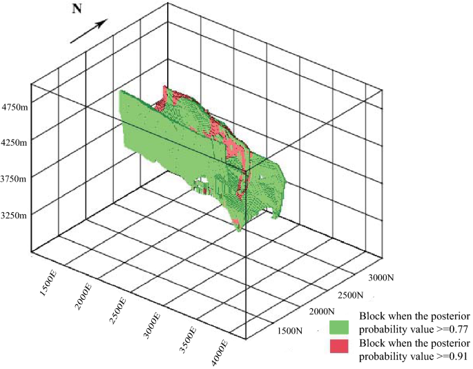

    

    Block when the posterior probability value is greater than or equal to 0.77, and 0.91

• 2. The information amount method is a statistical analysis method (Liu et al. 2012, 2013). It is based on various basic data, and the information value of each prediction factor is obtained through statistics. The information amount method is a nonparametric univariate statistical method. First, the prediction unit is divided. The study area is divided into several units of the same shape and size, and the geological elements are then determined. For the calculation, the element status data must be converted into two states (0, 1). Then, the conditional probability of the information amount of each prediction element is calculated, and the formula is as follows:

  $$ I_{A(B)} = \lg \frac{P(A/B)}{P(A)} $$

  (32)

  where I_A(B) is the amount of information for element A with ore body B; P(A/B) is the probability of the occurrence of element A when ore body B is known to exist; P(A) is the probability of occurrence of the element A in the entire study area. The probability value of the information amount is estimated by the frequency value.

  $$ I_{A(B)} = \lg \frac{{\left( {\frac{{N_{j} }}{N}} \right)}}{{\left( {\frac{{S_{j} }}{S}} \right)}} $$

  (33)

  where N_j is the number of units of ore bodies with element A in the study area; N is the number of units containing ore bodies in the study area; S_j is the number of units with element A in the study area; and S is the total number of units in the study area.

According to the Bayesian view and the uncertainty around such estimation, the more knowledge we have, the more certain we are about an outcome (Christakos 1990). First, the information factor in each block is defined. When geological information exists, the attribute takes a value of 1. If this information does not exist, the value is 0. The information quantities in different blocks are shown in Table 6. When the information amount is greater than or equal to 1.65, the ratio of the total number of ore bodies changes significantly. Therefore, the information amount threshold is selected to be 1.65. Figure 18 shows the block when the amount of information is greater than 1.65.

Table 6 Number of blocks and the ratio of the total number of ore bodies when the information takes different values

Figure 18

Block when the amount of information is greater than 1.65

Finally, using the two methods together to constrain the problem, the favorable area for ore formation is delineated based on the quantitative analysis of mineralization geological anomalies. Figure 19 shows the favorable areas delineated by the information threshold and the probability threshold.

Figure 19

Favorable areas delineated by the information threshold and the probability threshold

In addition, the authors analyze the metallogenic geological anomalies from the analytical results of the metallogenic process simulation. The prospective value for pore water pressure is between − 4.2e+7 and − 2.8e+7 Pa, and the volumetric strain value is between 8.33e−15 and 5.0e−14 m³.

Based on the above study of the geological mineralization characteristics of the study area, a 3D prediction model of the study area is established (Table 7). Marble is selected as a prime geological unit because it commonly hosts mineralization. The quantitative analysis of fractures and faults includes fracture analysis, local fracture analysis and structural center symmetry, and eigenvalues are obtained by the superposition analyses with known ore bodies, as shown in Table 7. In addition, the pore water pressure and the volumetric strain value also play very important roles in prediction and are very favorable ore-controlling factors.

Table 7 Prediction model for the Kaerqueka study area

From the prediction model developed for the study area, the authors conduct a combined prediction for mineral and metallogenic anomalies and define a prospective area for mineral deposits in the Kaerqueka mineral field by applying the information amount and WoE methods. This process reduces uncertainty and multiplicity in the metallogenic geological anomaly analysis. The result is an increased accuracy for the 3D study of “mineral potential mapping.”

Figure 20 shows the favorable ore-forming areas defined by the combined prediction superposed with marble and skarn. Figure 21 illustrates the favorable ore-forming areas delineated by combined prediction superposed with faults. Figure 22 shows target areas by combined prediction. The above analysis indicates that mineralization in the Kaerqueka mineral field is closely related to the intrusive bodies emplaced along major faults, especially where skarns occur at the contacts between marble and granodiorite.

Figure 20

Favorable ore-forming areas defined by combined prediction superposed with the location of marble and skarn in the Kaerqueka mineral field

Figure 21

Favorable ore-forming areas delineated by combined prediction superposed with faults

Figure 22

Target areas by combined prediction

Conclusions

Predicting the locations of the Kaerqueka deposit involves the combined analysis of metallogenic geological and mineralization geological anomalies, which provides a new way of 3D mineral potential mapping for concealed orebodies. This study draws the following conclusions:

• (a) Theoretical methods of hydrothermal mineralization simulation are systematically studied, and a stress–heat–fluid coupling simulation using FLAC3D is completed. The metallogenic geological anomalies of the study area are analyzed by metallogenic process simulation. The pore water pressure and the volumetric strain value play very important roles in 3D mineral potential mapping. When the prospective value for pore water pressure is between − 4.2e+7 and − 2.8e+7 Pa and the volumetric strain value is between 8.33e−15 and 5.0e−14 m³, a deposit is most likely to form. This method reduces the uncertainty of the mineralization geological anomaly analysis.

• (b) The 3D geological model constructed for the Kaerqueka deposit is established using the Surpac 3D modeling software, on which the mineralization geological anomaly analysis is completed. A posterior probability value of 0.77 is selected as the threshold, and the information amount threshold is selected as 1.65. Through the information amount and WoE methods, the favorable areas for ore formation are delineated. This method reduces the multiplicity of the metallogenic geological anomaly analysis.

• (c) The method is also applicable to other types of deposits. Note here that there are different solutions for deposits with different genetic models by changing variables such as temperature, flow quantity, pore water pressure and volumetric strain. Applying the mineralization geological anomaly analysis in 3D modeling, the combined mineralization prediction of concealed orebodies is effectively implemented. This method is widely used in “mineral potential mapping.”

References

Balashov, V. N., Yardley, B. W. D., & Lebedeva, M. (1999). Metamorphism of marbles: Role of feedbacks between reaction, fluid flow, pore pressure and creep. In B. Jamtveit & P. Meakin (Eds.), Growth, dissolution and pattern formation in geosystems (pp. 367–380). Dordrecht: Springer.
Batley, G. E., Burton, G. A., Chapman, P. M., & Forbes, V. E. (2002). Uncertainties in sediment quality Weight-of-Evidence (WOE) assessments. Human and Ecological Risk Assessment,8(7), 1517–1547.
Busse, F. H., Christensen, U., Clever, R., Cserepes, L., Gable, C., Giannandrea, E., et al. (1994). 3D convection at infinite Prandtl number in Cartesian geometry: A benchmark comparison. Geophysical Fluid Dynamics,75(1), 39–59.
Che, G.-X., & Xue, C.-J. (2011). Principles, methods and applications of hydrodynamic studies of mineralization. Earth Science Frontiers,18(5), 1–18.
Chen, B., Zhang, Z., Geng, J., Jian, Q., Song, Z., Zhao, X., et al. (2012). Zircon LA-ICP-MS U-Pb age of monzogranites in the kaerqueka copper-polymetallic deposit of Qimantag, western Qinghai province. Geological Bulletin of China,31, 463–468.
Chen, J., Jie, X., Qiao, H. U., Wei, Y., Lai, Z., Bin, H. U., et al. (2016). Quantitative geoscience and geological big data development: A review. Acta Geologica Sinica,90(4), 1490–1515.
Chen, J., Lu, P., Wu, W., Zhao, J., & Hu, Q. (2007). A 3-D prediction method for blind orebody based on 3-D visualization model and its application. Earth Science Frontiers,14(5), 54–61.
Chen, J., Yu, P., Shi, R., Yu, M., & Zhang, S. (2014). Research on three-dimensional quantitative prediction and evaluation methods of regional concealed ore bodies. Earth Science Frontiers,21(5), 211–220.
Christakos, G. (1990). A bayesian/maximum-entropy view to the spatial estimation problem. Mathematical Geology,22(7), 763–777.
Du, S., He, Y.-L., Yang, W.-W., & Liu, Z.-B. (2018). Optimization method for the porous volumetric solar receiver coupling genetic algorithm and heat transfer analysis. International Journal of Heat and Mass Transfer,122, 383–390.
Garven, G. (1985). The role of regional fluid flow in the genesis of the pine point deposit, western Canada sedimentary basin. Economic Geology,80(2), 307–324.
Gold, V. (1988). Compendium of chemical terminology. Journal of Organometallic Chemistry,356(2), C76–C77.
Gong, J.-W., Xi, X.-W., Wang, Y.-J., & Lin, G. (2002). Numerical model method of stress and strain—introduce to numerical model software FLAC. Journal of East China Geological Institute,25(3), 220–227.
Götze, H. J., El-Kelani, R., Schmidt, S., Rybakov, M., Hassouneh, M., Förster, H. J., et al. (2007). Integrated 3D density modelling and segmentation of the Dead Sea Transform. International Journal of Earth Sciences,96(2), 289–302.
Griffin, D., & Tversky, A. (1992). The weighing of evidence and the determinants of confidence. Cognitive Psychology,24(3), 411–435.
Harff, J., Watney, W. L., Bohling, G. C., Doveton, J. H., Olea, R. A., & Newell, K. D. (2001). Three-dimensional regionalization for oil field modeling. In D. F. Merriam & J. C. Davis (Eds.), Geologic modeling and simulation. Computer applications in the earth sciences (pp. 205–227). Boston, MA: Springer.
Hobbs, B. E., Zhang, Y., Ord, A., & Zhao, C. (2000). Application of coupled deformation, fluid flow, thermal and chemical modelling to predictive mineral exploration. Journal of Geochemical Exploration,69–70, 505–509.
Jianping, C., Yong, C., Min, Z., Zhongde, H., Jie, Z., Qing, H., et al. (2008). 3D positioning and quantitative prediction of the Koktokay No. 3 pegmatite dike, Xinjiang, China, based on the digital miner of deposit model. Geological Bulletin of China,27(4), 552–559.
Khramchenkov, E., & Khramchenkov, M. (2018). Numerical model of two-phase flow in dissolvable porous media and simulation of reservoir acidizing. Natural Resources Research,27(4), 531–537.
Lee, C., Oh, H.-J., Cho, S.-J., Kihm, Y. H., Park, G., & Choi, S.-G. (2018). Three-dimensional prospectivity mapping of skarn-type mineralization in the southern Taebaek area, Korea. Geosciences Journal,23(2), 327–339.
Li, D.-S., Gu, F.-B., Zhang, H.-L., Su, S.-S., Zhong, L.-Y., & Liu, G.-L. (2012). Geologic characteristics of the kaerqueka porphyry copper deposit in Qinghai province and its prospecting significance. Northwestern Geology,45(1), 174–183.
Li, D. S., Zhang, Z. Y., Su, S. S., Guo, S. Z., Zhang, H. L., & Kui, M. J. (2010). Geological characteristics and genesis of the Kaerqueka copper molybdenum deposit in Qinghai province. Northwestern Geology,43(4), 239–244.
Li, D. X., Feng, C. Y., Zhao, Y. M., Li, Z. F., Liu, J. N., & Xiao, Y. (2011). Mineralization and alteration types and skarn mineralogy of Kaerqueka copper polymetallic deposit in Qinghai province. Journal of Jilin University,41(6), 1818–1830.
Li, N., Song, X., Xiao, K., Li, S., Li, C., & Wang, K. (2018). Part II: A demonstration of integrating multiple-scale 3D modelling into GIS-based prospectivity analysis: A case study of the Huayuan-Malichang district, China. Ore Geology Reviews,95, 292–305.
Li, S., Sun, F., Wang, L., Li, Y., Liu, Z., Su, S., et al. (2008). Fluid inclusion studies of porphyry copper mineralization in Kaerqueka polymetallic ore district, east Kunlun Mountains, Qinghai province. Mineral Deposits,27(3), 399–402.
Liu, Y., Tang, C., & Feng, Y. (2013). Geological disaster risk assessment based on AHP information method. Earth and Environment,41(2), 173–179.
Liu, Z.-F., Shao, Y.-J., Shu, Z.-M., Peng, N.-H., Xie, Y.-L., & Zhang, Y. (2012). Fluid inclusion characteristics of Longmenshan copper-polymetallic deposit in Yueshan, Anhui province, China. Journal of Central South University,19(9), 2627–2633.
Mao, X., Zhang, M., Deng, H., Zou, Y., & Chen, J. (2016). Three-dimensional visualization prediction method for concealed ore bodies in deep mining areas. Journal of Geology,16(3), 612–618.
Nielsen, S. H. H., Cunningham, F., Hay, R., Partington, G., & Stokes, M. (2015). 3D prospectivity modelling of orogenic gold in the Marymia Inlier, western Australia. Ore Geology Reviews,71, 578–591.
Niemann, M., Navarro, R. A. B., Saini, V., & Fröhlich, J. (2018). Buoyancy impact on secondary flow and heat transfer in a turbulent liquid metal flow through a vertical square duct. International Journal of Heat and Mass Transfer,125, 722–748.
Norton, D. L., & Hulen, J. B. (2001). Preliminary numerical analysis of the magma-hydrothermal history of the geysers geothermal system, California, USA. Geothermics,30(2–3), 211–234.
Ord, A., & Oliver, N. H. S. (2010). Mechanical controls on fluid flow during regional metamorphism: Some numerical models. Journal of Metamorphic Geology,15(3), 345–359.
Øren, P.-E., & Bakke, S. (2002). Process based reconstruction of sandstones and prediction of transport properties. Transport in Porous Media,46(2/3), 311–343.
Potma, W., Roberts, P. A., Schaubs, P. M., Sheldon, H. A., Zhang, Y., Hobbs, B. E., et al. (2008). Predictive targeting in Australian orogenic-gold systems at the deposit to district scale using numerical modelling. Australian Journal of Earth Sciences,55(1), 101–122.
Qu, J., & Deutsch, C. V. (2017). Geostatistical simulation with a trend using gaussian mixture models. Natural Resources Research,27(3), 347–363.
Schaubs, P. M., Rawling, T. J., Dugdale, L. J., & Wilson, C. J. L. (2006). Factors controlling the location of gold mineralisation around basalt domes in the stawell corridor: Insights from coupled 3D deformation-fluid-flow numerical models. Australian Journal of Earth Sciences,53(5), 841–862.
Seng, D., Li, Z., & Li, C. (2004). 3D visual modeling system for mineral deposits. Journal of University of Science and Technology Beijing,26, 453–456.
Sheldon, H. A. (2009). Simulation of magmatic and metamorphic fluid production coupled with deformation, fluid flow and heat transport. Computers and Geosciences,35(11), 2275–2281.
Sides, E. J. (1997). Geological modelling of mineral deposits for prediction in mining. Geologische Rundschau,86(2), 342–353.
Stavropoulou, M., Exadaktylos, G., & Saratsis, G. (2007). A combined three-dimensional geological-geostatistical-numerical model of underground excavations in rock. Rock Mechanics and Rock Engineering,40(3), 213–243.
Takafuji, E. H. D. M., Rocha, M. M. D., & Manzione, R. L. (2018). Groundwater level prediction/forecasting and assessment of uncertainty using SGS and ARIMA models: A case study in the Bauru aquifer system (Brazil). Natural Resources Research,28(2), 487–503.
Tkachev, A. V., & Rundqvist, D. V. (2016). Global trends in the evolution of metallogenic processes as a reflection of supercontinent cyclicity. Geology of Ore Deposits,58(4), 263–283.
Van Dijk, J. P. (1993). Three-dimensional quantitative restoration of central Mediterranean Neogene basins: The dynamic geohistory approach. In A. M. Spencer (Ed.), Generation, accumulation and production of Europe’s hydrocarbons III. Special publication of the European association of petroleum geoscientists (pp. 267–280). Berlin, Heidelberg: Springer.
Wellmann, J. F., & Regenauer-Lieb, K. (2012). Uncertainties have a meaning: Information entropy as a quality measure for 3-D geological models. Tectonophysics,526–529, 207–216.
Xie, H.-P., Zhou, H.-W., Wang, J.-A., Li, L.-Z., & Kwasniewski, M. A. (1999). Application of FLAC to predict ground surface displacements due to coal extraction and its comparative analysis. Chinese Journal of Rock Mechanics and Engineering,18(4), 397–401.
Xie, J., Wang, G., Sha, Y., Liu, J., Wen, B., Nie, M., et al. (2016). GIS prospectivity mapping and 3D modeling validation for potential uranium deposit targets in Shangnan district, China. Journal of African Earth Sciences,128, 161–175.
Xinbiao, L., & Pengda, Z. (1998). Geologic anomaly analysis for space-time distribution of mineral deposits in the middle-lower Yangtze area, Southeastern China. Nonrenewable Resources,7(3), 187–196.
Zhang, Y., Zhang, D., Liu, G., Li, Z., Zhao, Y., Li, H., et al. (2017). Zircon U-Pb dating of porphyroid monzonitic granite in the Kaerqueka copper polymetallic deposit of east Kunlun Mountains and its geological significance. Geological Bulletin of China,36, 270–274.
Acknowledgments
First, we thank Yan Sun for her linguistic contributions to this paper. Second, we acknowledge the contributions of the Surpac and FLAC3D software packages in geological modeling. Finally, we also appreciate Leon Bagas’s help with the grammar modification. We are grateful to all the reviewers for their work in our manuscript, and the opinions of reviewers have helped us a lot. This research was financially supported by the National Key Research and Development Program of China (NKRDPC, Project No. 2017YFC0601502).
Author information
Authors and Affiliations
Corresponding author
Rights and permissions
Open Access This article is distributed under the terms of the Creative Commons Attribution 4.0 International License (http://creativecommons.org/licenses/by/4.0/), which permits unrestricted use, distribution, and reproduction in any medium, provided you give appropriate credit to the original author(s) and the source, provide a link to the Creative Commons license, and indicate if changes were made.
About this article
Cite this article
Wang, Y., Chen, J. & Jia, D. Three-Dimensional Mineral Potential Mapping for Reducing Multiplicity and Uncertainty: Kaerqueka Polymetallic Deposit, QingHai Province, China. Nat Resour Res 29, 365–393 (2020). https://doi.org/10.1007/s11053-019-09539-9
Received:
Accepted:
Published:
Issue Date:
DOI: https://doi.org/10.1007/s11053-019-09539-9