A novel COVID diagnosis and feature extraction based on discrete wavelet model and classification using X-ray and CT images

Abstract

Recently, the Covid-19 pandemic has affected several lives of people globally, and there is a need for a massive number of screening tests to diagnose the existence of coronavirus. For the medical specialist, detecting COVID-19 cases is a difficult task. There is a need for fast, cheap and accurate diagnostic tools. The chest X-ray and the computerized tomography (CT) play a significant role in the COVID-19 diagnosis. The advancement of deep learning (DL) approaches helps to introduce a COVID diagnosis system to achieve maximum detection rate with minimum time complexity. This research proposed a discrete wavelet optimized network model for COVID-19 diagnosis and feature extraction to overcome these problems. It consists of three stages pre-processing, feature extraction and classification. The raw images are filtered in the pre-processing phase to eliminate unnecessary noises and improve the image quality using the MMG hybrid filtering technique. The next phase is feature extraction, in this stage, the features are extracted, and the dimensionality of the features is diminished with the aid of a modified discrete wavelet based Mobile Net model. The third stage is the classification here, the convolutional Aquila COVID detection network model is developed to classify normal and COVID-19 positive cases from the collected images of the COVID-CT and chest X-ray dataset. Finally, the performance of the proposed model is compared with some of the existing models in terms of accuracy, specificity, sensitivity, precision, f-score, negative predictive value (NPV) and positive predictive value (PPV), respectively. The proposed model achieves the performance of 99%, 100%, 98.5%, and 99.5% for the CT dataset, and the accomplished accuracy, specificity, sensitivity, and precision values of the proposed model for the X-ray dataset are 98%, 99%, 98% and 97% respectively. In addition, the statistical and cross validation analysis is conducted to validate the effectiveness of the proposed model.

1 Introduction

Nowadays, COVID-19 is a global dangerous disease [18]. In December 2019, COVID-19 declared a new viral disease in China. The WHO declared coronavirus a pandemic disease in March 2020. Because of its high contagious characteristics spread over more than 225 countries with approximately 300 million confirmed cases and 4.3 million death cases. Among all recorded pandemics, this COVID-19 pandemic ranks second in deaths after the 1918 flu pandemic. Initially, the coronavirus affects the human throat and gradually moves to the respiratory organ. It spreads completely through the lungs, leading to high fever and sore throat and causing pneumonia. Loss of smell and taste, fever, dry cough, fatigue, malaise and shortness of breath are the major symptoms of the viral disease. The main symptoms of the coronavirus disease are. It can be complicated for the person suffering from chronic diseases such as respiratory diseases, high blood pressure, diabetes, autoimmune diseases and cardiovascular diseases.

The COVID-19 diagnosis using X-ray or X-radiation images of the chest has been described as an accurate diagnostic strategy [36]. To produce the images for the internal details of the human parts, these x-rays are passed to the desired parts of the human body. The internal human parts are represented in black and white shades in the x-ray images. The most common and one of the oldest medical diagnostic tests is the x-ray. The chest-related diseases such as pneumonia and other lung-related diseases are diagnosed using chest x-ray. It also provides pictures of the thoracic cavity, which contains chest and spine bones with soft organs like lungs, airways, and blood vessels [37]. X-ray imaging methods offer enormous advantages over other test methods for diagnosing COVID-19. These advantages include low cost complexity, non-invasiveness, the vast availability of x-ray, device affordability and consuming less time. Hence, the x-ray imaging technique is the best procedure for easy and quick COVID-19 diagnosis.

Computed tomography (CT) and radiography are considered integral players in the COVI-19 preliminary diagnosis. Thus, the enormous number of patients and inadequate radiologists relatively increase the false positive rate. Modern computer-aided chest CT diagnosis strategies are required urgently for confirming suspected cases, conducting virus surveillance and screening patients accurately [33]. The most commonly used AI techniques to diagnose the COVID-19 X-ray or CT images in CNN are VGG-16, VGG-19, ResNet50V2, ResNet18, ResNet 50, AlexNet LeNet-5 and CoroNet [24]. In addition, Canayaz proposed hybrid DNN-metaheuristic optimizers for the COVID-19 diagnosis. Three sets of x-ray images are considered: normal, pneumonia and COVID-19, it was utilized to train the model. The contrast enhancement procedure is used for the image pre-processing. The methods like VGG19, ResNet, GoogLeNet and AlexNet are used for feature extraction [28]. The metaheuristic optimizer particle swarm and the grey wolf are used to select the best features. Over the wide range of applications domain, namely, speech recognition, biological science, NLP, image processing etc., the ANN has proved its existing techniques in these areas.

At present, Machine learning (ML) and deep learning (DL) techniques have made very better enhancements to the diagnosis of diseases automatically and also made it low cost and more accessible [43]. It provides maximum performance for various image processing applications, namely, image analysis, classification, and segmentation. The descriptor extracts important features from the images for image classification. The example for descriptors is SIFT, image moment. The SVM classifier uses these extracted features in the classification work [43].

On the other hand, deep neural network-based techniques also provide maximum performance in image classification based on the extracted features. Another ML/metaheuristic optimizing scheme was introduced to diagnosis COVID-19 infections with the help of x-ray images. The fractional exponent moments algorithm extracted the significant features from the processed images. Here, the multicore computational strategy was used to accelerate the computational process of the developed algorithm. Then the significant features are chosen by the hybrid manta-ray foraging or differential evolution optimizer [22]. Depending on the characteristics of ML, various efforts used ML-based approaches to classify the x-ray image of the chest as a normal or abnormal class.

Further, the hybrid marine predators’ optimizer and the moth-flame optimizer are utilized to segment the images of COVID-19 cases [27]. To eliminate the falling into local optima, the latter optimizer is considered the subroutine in the former optimizer. The proposed method works better than the other modern optimizers such as particle swarm optimization, standalone marine predator’s optimizer, grey wolf optimizer, spherical search optimizer, Harris hawks optimizer, moth-flame optimizer, cuckoo search optimizer and grasshopper algorithm. To classify the COVID-19 x-ray images as normal, COVID-19 and pneumonia using the cuckoo search and fractional calculus algorithm optimizer. Four heavy-tailed distributions, such as the Weibull distribution, Cauchy distribution, Pareto distribution and Mittag-Leffler distribution, were used to robust the proposed method’s performance.

In [17], a particle swarm optimization based segmentation technique was proposed for segmenting prostate cancer (PCa) with the aid of multi-parametric MRI images. The accomplished accuracy was 7.6%, but the gradient descent increases the computational overhead. Further [13], TRUS, MRI and CT are some modalities used to diagnose the PC as efficiently. Since several denoising methods are available but the removal of noise was still a challenging task. So analysis is performed over the various modality images in the gaussian and rician noise environment [16]. In early cancer detection, PCa patients’ accurate and timely diagnosis plays a significant role [14]. Therefore, various cancer localization methods are used for segmenting prostate zonal. For the detection of PCa, some classification, clustering, and probabilistic methods [15] are available for accurate diagnosis.

Artificial intelligence provides maximum performance for automated image classification problems using various ML techniques. It takes classification decision depends on the vast quality of data samples. DL is a set of ML schemes whose major focus is automated extraction and classification of image features and provides accurate results, particularly in health care. Various AI techniques are utilized to find the optimal network for the domain of researchers. Convolutional neural networks (CNNs) and recurrent neural networks (RNN) are the two famous DL based networks that are significantly used in the COVID-19 detection domain [38]. The pre-processing, feature extraction and classification of x-ray and CT images using CNN have shown accurate results in medical image processing. Due to the low cost, high operating speeds and easy use, the x-ray and CT scan images play a significant role in the COVID-19 detection and classification techniques.

One of the most famous and proficient models is the Deep neural network (DNN) which is used in various areas such as speech analysis, computer vision, robotic control, etc. In DNN, Popular Graphical Processing Units (GPUs) and large scale datasets are used to extract the significant features from the datasets. However, the classification performance of the proposed DNN model is inaccurate [39]. So, the researchers implement DNNs in AI analysis techniques for COVID-19 diagnosis. In [20], a non-overlapping detection algorithm (OR-ACM) was applied for segmenting the normal and abnormal cells. After that, the features are extracted with the aid of HOG and color moments. Then multi-objective classifier (M-SVM) is utilized to characterise the normal and abnormal images. The adaptive regularised Kernel fuzzy C-means scheme is used for classifying the cells, and the distance among the derived outcomes is computed with earth movers distance [19]. Among many researchers, the Content based medical image retrieval (CBMIR) system gained more attention. So, an effective Hybrid feature based independent condensed nearest neighbour model is introduced to classify the seven cell classes [35].

Moreover, the k-nearest neighbours algorithm was proposed to accelerate classification performance by selecting necessary features and eliminating irrelevant ones [42]. Furthermore, most of the COVID-19 classification techniques have disadvantages that affect the classification’s accuracy rate. These limitations occur due to either the scheme utilized for feature extraction or the strategy used to minimize the number of selected features.

Several detection schemes have been introduced to handle the spread of COVID-19, but implementing various ML/DL techniques to detect and classify COVID-19 is insufficient. The ML-based approaches require a large amount of data for designing the detection models. The DL techniques only provide better outcomes and reasonable solutions to handle pandemic situations if a limited amount of medical images are available. Medical image mining consumes a lot of time and is costly, and there is a need for the involvement of researchers and radiologists. COVID-19 ML based screening models faced spatial information loss, which is still a significant concern.

Many researchers are fascinated with the DL based CNN model, but it is also very difficult and challenging [41]. The CNN model needs a large number of training data, leading to various disadvantages, making the process more complex and consuming more time. To diagnose COVID-19, innovative advanced technology is needed to achieve high accuracy. Peripheral research is also conducted here, still, major disadvantages arise in the COVID-19 diagnosis.

The limitations mentioned above motivate us to propose an excellent DL architecture such as a modified discrete wavelet based Mobile Net model for feature extraction and classification purpose. This proposed model undergoes three stages: pre-processing, feature extraction, and classification. In the pre-processing stage, the unwanted noises are eliminated using the MMG hybrid filtering approach, which integrates mean, median and Gaussian filters. The next stage is feature extraction, the first and second-order statistical texture features are collected from the pre-processed images. The modified Mobile Net model is introduced in this feature extraction stage to extract the respective features from the collected output of the pre-processing stage. The higher dimensionality of the feature vectors affects the proposed model’s performance, so to reduce the dimensionality of the feature vectors wavelet approach is introduced. It optimizes the downsampling function without affecting the spatial information of images. The third stage is the classification, in this phase convolutional Aquila COVID detection neural network model is proposed. The Aquila optimizer is used effectively to minimize the loss function. For the proposed technique, 6432 chest x-ray images and 349 CT scans images are present in the datasets to achieve efficient classification performance with the aid of the proposed DL model. Finally, the classification of normal and COVID-19 cases results are obtained accurately. Our proposed work undergoes the below mentioned major contributions, which are:

• This research aims to design an efficient, optimised DL model to estimate COVID-19 from the X-ray and CT images. The research intended a hybrid MMG approach to remove the noise and enhance the quality of the images in the pre-processing stage.

• The proposed model employs a modified discrete wavelet based Mobile Net for extracting first and second order statistical features. The wavelet approach is used to reduce the dimensionality of the feature and achieve more accurate results. It also helps accelerate the training process’s speed and avoids gradient issues.

• COVID and non-COVID are classified with the aid of the proposed convolutional Aquila COVID detection neural network. The introduced Aquila optimizer reduced the loss function and fine-tuned the hyperparameters.

• Extensive experiments are performed using the X-ray and CT dataset with a performance comparison of the introduced model and previous approach for classifying COVID-19 images. In addition, the Wilcoxon signed-rank test was done to access the statistical significance, and the cross validation analysis was conducted.

The upcoming sections are explained in detail below: Section 2 discusses the state-of-art techniques related to detecting COVID-19. Section 3 includes the proposed methods. Section 4 explains the result and discussion. Section 5 discusses the conclusion of the proposed method.

2 Related works

Currently, coronavirus has been considered to be a pandemic disease. This disease’s symptoms are pneumonia, which affects the respiratory organs. The real-time reverse transcriptase polymerase chain reaction (RT-PCR) kit is used to diagnose COVID-19. Due to the unavailability of the kits, it takes too long to find the availability of a person affected by the virus. So that the affected person cannot be treated in time, to solve this problem, Nigam et al. [32] proposed a famous DL architecture for the coronavirus diagnostic systems. VGG16, xception, denseNet121, efficient net, and NASnet are the architecture used in this paper. The multi-class classification was done here; the classes are normal, COVID-19, pneumonia, influenza and other sicknesses. The achieved accuracy level of the VGG16 is 79.01%, denseNet121 is 89.96%, xception is 88.03%, NASnet is 85.03%, and the efficient net is 93.48%. The only drawback is that the amount of images used for COVID-19 patients is low.

Chen [6] introduced an accurate classification model to diagnose the COVID-19 disease. The CNN classification model proposed for the medical images depends on various edge based neural networks. If the number of classes increases in the training network, the tertiary classification accuracy decreases. To detect the different diseases caused by the lung infection, the analysis of 10 fold cross-validation and confusion matrix is also performed in this work. The proposed model was trained and tested using public X-ray datasets. The achieved accuracy level of the proposed CNN-based tertiary classification is 85%, including normal, abnormal, and pneumonia. But the limitation faced in this paper was to identify COVID-19 from a specific amount of images without performing the pre-processing stage.

Demir [9] defined an innovative method based on a deep LSTM model to immediately detect the COVID-19 cases from the x-ray images. Resource shortages like test kits and ventilators arised in many countries due to the increase in COVID-19 cases. Differing from the transfer learning and deep feature extraction strategy, the deep LSTM model is learned from scratch. In the pre-processing step, the proposed method performance was increased by using the marker-controlled watershed segmentation function, and the Sobel gradient was done to the raw pictures. The classes considered in this proposed work were normal, COVID-19, pneumonia and chest x-ray images. Based on training and testing, the dataset is classified. The best training performance is 80%, and the testing is 20%.

Further, a 100% success rate was obtained for every performance criterion, including accuracy, specificity, sensitivity and F-score. The introduced method significantly enhances the available radiology-based process and is very useful for specialists and radiologists to diagnose COVID-19. The drawback of this proposed model was that it needs high memory bandwidth for real-time applications.

Kumar et al. [30] proposed the hybrid convolutional neural network (HDCNN), which fuses convolutional neural network (CNN) and recurrent neural network (RNN) structure for detecting COVID-19 cases by utilizing chest x-ray images. With the increase in COVID-19 cases and X-rays, it is necessary to classify the x-ray with the help of transfer learning. The slope weighted activation class planning (Grad-CAMs) was used as a transfer learning method to identify whether the person was affected by the coronavirus or not with the HDCNN architecture. The accomplished accuracy, precision, recall and F1-score values are: 98.20%, 97.31%, 97.1%, 0.97 respectively. This method suffers due to the RNN classification i.e.it classifies the input signal with raw data into 700 steps and 64 units for every step, which leads to learning complexity.

Elaziz et al. [1] proposed COVID-19 image classification based on MobileNetV3 and Aquila optimizer algorithm. Here, the MobileNetV3 is utilized to extract the significant features from the feature set of DL model. Secondly, the Aquila optimizer is a swarm-based technique used to minimize the dimensionality of the feature vectors. It is done via two stages: learning the model and estimating the selected features. Finally, the accomplished accuracy, recall, precision and f1-score of this proposed algorithm for the dataset1 are 0.783, 0.783, 0.785, 0.782 and for dataset2 are 0.974, 0.974, 0.974 and 0.974 respectively.

Shankar et al. [40] implemented fusion-based feature extraction to diagnose COVID-19 using chest x-ray images. This proposed method undergoes three stages: pre-processing, feature extraction and classification. Frist of all, the Weiner filtering method (WFM) is used to perform the preprocessing of the images. Secondly, the gray level co-occurrence matrix (GLCM), gray level run length matrix (GLRM), and local binary patterns (LBP) features are fused by the fusion based feature extraction procedure.

Then the optimal features are extracted by salp swarm optimization (SSA), a random population-relied technique. Finally, the ANN architecture of multilayer perceptron (MLP) efficiently classifies the various classes of COVID-19. The achieved sensitivity, specificity, accuracy and f1-score value of FM-ANN are 95.65%, 95.94%, 95.70% and 95.35%, correspondingly.

Ahsan et al. [3] proposed diagnosis of COVID-19 from the chest x-ray images based on feature fusion and deep learning. It achieves maximum accuracy and minimum complexity by integrating the extracted features through CNN and histogram-oriented gradient (HOG). The modified anisotropic diffusion filtering (MADF) was introduced to minimize noise and preserve the images’ edges. Finally, the classification was done by the CNN (VGGNet19). The obtained testing accuracy, specificity and sensitivity are 99.49%, 95.7% and 93.65%, respectively, clearly showing the proposed algorithm’s effectiveness.

Elpeltagy and Sallam [12] implemented the modified ResNet50 was introduced to classify the patients as COVID-19 affected and normal cases. Here, the modification consists of three layers: Conv, Batch_Normaliz and Activation_Relu. It leads to extracting more robust features and enhancing classification accuracy.

Elmuogy et al. [11] developed a Worried Deep Neural Network (WDNN), an automatic classification structure based on DNN. This proposed model was used to classify the COVID-19 virus from the CT images based on some pre-trained models such as Inception v3, Resnet(50), and VGG(19). These three architectures efficiently extract and classify features from pictures. The performance measures of accuracy, precision, recall and F1-score are evaluated. Table 1 represents the recent works of COVID-19 classification.

Table 1 Comparision with state-of art techniques

Problem formulation

Detecting COVID-19 at the initial stage by imaging modalities may help to recover from the disease. Medical imaging modalities such as CT (computed tomography), (MRI (magnetic resonance imaging), ultrasound, and X-ray are utilized for examining the internal organs of the body and tissues. The existing methods are highly suffered because of various drawbacks, resulting in a very low accuracy level in the classification stage. In [32], DL architecture introduces coronavirus diagnostic systems. The drawback faced in this proposed system is that the number of images used for detecting COVID-19 is less. In [6], CNN classification model for diagnosing the COVID-19 disease. However, due to the lack of pre-processing, it has maximum noise in the feature extraction step. The main disadvantage of this proposed model based on CNN is that a certain number of images did not go through the pre-processing phase.

Further, in [9], the deep LSTM model to automatically detect COVID-19 cases needs an enormous memory bandwidth in the real-time application. It leads to cost complexity and needs lots of processing time to extract the features. In [30], an HDCNN is proposed that includes CNN and RNN for detecting COVID-19 cases. The classification stage classifies the input data into 700 steps and 64 for each step, which may cause learning complexity. So it doesn’t provide maximum accurate results.

Further, the images obtained from these modalities suffer from noise and artifacts. The noisy CT images have less contrast, and removing noise is challenging. Image pre-processing algorithms have been introduced to tackle these issues and enhance the image quality for better analysis and understanding. Sometimes overfitting risk may occur in the feature extraction phase, so an efficient feature extraction technique is needed. Hence, in this work, CNN based feature extraction model is carried out. After feature extraction, it is necessary to classify the image as diseased. The medical experts are trying not only to increase the image quality but also to classify the disease as COVID-19 or not. Our research introduced an efficient model to obtain maximum accuracy and high-performance speed. To the best of our awareness, our developed model is the significant research carried out in this platform will produce better accuracy and optimize the errors.

3 Proposed methodology

The chief goal of this research is to propose a COVID-19 diagnosis and feature extraction model with a wavelet based optimized network model. The enormous increase in COVID-19 cases and insufficient RT-PCR kit facilities delay testing and treating the patients. Fast and affordable computer-aided diagnosis techniques using x-ray and CT images can help medical practitioners detect viral disease early. This proposed methodology is classified into three phases. The model consists of pre-processing, feature extraction and classification. Initially, the data are collected from the dataset called COVID-XRay-6432 and CT. In the pre-processing phase, the MMG hybrid filtering technique is employed extensively for noise removal, smoothing, and enhancing the image’s quality. This MMG hybrid filtering integrates mean, median and Gaussian filters to obtain more accurate data. In the second phase, feature extraction is performed by introducing an innovative model named a modified discrete wavelet-based Mobile Net model with the help of this modified network model. From the pre-processed images, features are extracted, and the wavelet-based approach is introduced to diminish the dimensionality of feature vectors. Finally, in the classification stage, the convolutional Aquila neural network is developed for the training and testing in the classification phase. To reduce the loss function and fine-tune the hyperparameters using the effective new Aquila optimizer algorithm. This will improve the COVID detection accuracy effectively. Figure 1 shows the framework of the proposed methodology.

Fig. 1

Framework for the proposed methodology

3.1 Pre-processing

Medical images are get affected by several sources of artifacts and distortion. So, the visual evaluation of these pictures by radiologists becomes a challenging task. Also, the performance of a model gets degraded if the x-ray and CT scan datasets are constructed with various duplicates, obscure, blur etc. Therefore, performing initial tasks in the pre-processing stage is mandatory and necessary over a redundant image to acquire a better outcome.

In this pre-processing stage, the raw images are converted into a suitable format for further processing. The images gathered from the COVID-XRay and CT scan dataset may vary in size, some scans and slice thickness. These parameters produce a heterogeneous collection of imaging data, leading to non-uniformity over the datasets. So, in the pre-processing stage, have to perform image resizing, normalization, sometimes transforming the RGB images to grayscale images, noise elimination, smoothing and enhancing the quality of the images. For this, a new MGG hybrid filtering technique combines mean, median and gaussian filters. This MGG hybrid filtering approach performs the image smoothening and noise removal without any deviation from the images.

The MMG hybrid filtering technique is utilized in this research work by integrating mean, median and Gaussian filtering techniques. Due to this reason, a clear explanation for mean, median and Gaussian filtering techniques is given as follows.

3.1.1 Mean filter (MF)

The mean filter is otherwise known as the average filter, it enhances the pixel value in a picture with the aid of mean values of the gray scale in the neighbpurhood. This filtering technique is very simple and easy to implement. The images get enhanced by minimizing the changes in the image’s pixel intensities. It is generally used for blurring and smoothing the image, which minimizes the noises in the images [31]. The mathematical expression for the MF technique is given as follows.

$$ G\left(p,q\right)=\frac{1}{n^{\ast }m}\sum \limits_{a,b\in {N}_{pq}}H\left(a,b\right) $$

(1)

Where, the parameter N_pq is represented as neighbourhood sub image centered at a point (p, q) and window of size n × m. In H, the gray level of a pixel is (p, q), the term G(p, q) be the gray level which is replaced by the environmental pixel account information by the mean filter.

3.1.2 Median filter (MEF)

MEF is a nonlinear smoothing filter utilized to eliminate the salt-and-pepper noise from the image [29]. Initially, in ascending order, all the sliding window entries get sorted. Two cases are present in this MEF filtering technique: odd number of entries and even number of entries. If the number of entries is m. The mathematical model for an odd number of cases is written as,

$$ Median(Me)={\left(\left(m+1\right)/2\right)}^{th} $$

(2)

Otherwise, in the even number of entries, the mathematical expression can be given as,

$$ Median(Me)=\left({\left(m/2\right)}^{th}+{\left(m/2+1\right)}^{th}\right)/2 $$

(3)

The two types of MEF are maximum filter and minimum filter. In the maximum filter, the highest pixel value is chosen from the window. The minimum filter selects the lowest pixel value from the window.

3.1.3 Gaussian filter (GF)

The Gaussian filter is a 2D convolution operator highly utilized to eliminate noise and smoothen the images. The convolution of an image ϖ(a, b) with the function F(a, b) of size p × q. It is mathematically denoted as,

$$ \varpi \left(a,b\right)\ast F\left(a,b\right)=\sum \limits_{r=-x}^x\sum \limits_{s=-y}^y\varpi \left(r,s\right)F\left(a-r,b-s\right) $$

(4)

Where, x is mentioned as $x=\frac{p-1}{2}$ and y is mentioned as $y=\frac{q-1}{2}$.

The GF is a low-pass filter significantly used in image processing platforms to eliminate noise in the image. In this GF, blurring and smoothening are performed to enhance the image’s quality and eliminate noise. Different image processing applications like image blurring and edge detection are performed very easily using the Gaussian filtering approach. The function F(a, b) states the GF and is indicated by the Gaussian distribution. The mathematical formula for GF is mentioned below [5].

$$ Ga(x)=\frac{1}{\sqrt{2{\pi \alpha}^2}}{e}^{\frac{x^2}{2{\alpha}^2}} $$

(5)

Where α denotes the standard deviation of Gaussian distribution. The value of α is maximum means the image smoothing will also be maximum. Based on the spatial and frequency domain perspective, these GFs are considered effective low pass filters.

The drawback of mean filtering is significantly distorted the pixel average, leading to significant improvement in the reduction of noise; moreover, the image is blurred. The disadvantage of median filtering is insufficient to eliminate the high density impulse noise. The demerit of the Gaussian filter is that it takes too much time and reduces the image’s detail to overcome this kind of issue. The proposed MMG pre-processing techniques are used to solve these kinds of issues. The advantages of MMG filters are that they correct the pixel’s intensity to eliminate appreciable variations among the different sets of images. This hybrid approach eliminates the duplicate or inconsistencies of images because it degrades the model’s accuracy level. It enhances the image features significantly for further processing. The fully connected layers in CNN need all images to be in equal sized arrays, this MMG filter efficiently performs it to obtain a better outcome. Also, it minimizes the system training time and maximizes system inference time due to the hybridization of mean, median and gaussian techniques.

3.1.4 MMG hybrid filtering technique

At first, determine the kernel matrix size by utilizing the sample image. This section, considering 3 × 3 kernel matrix using this kernel matrix size, applied the mean median and Gaussian on the sample image. Calculate the same pixels output vector from the images that apply mean, median and Gaussian filtered and produce a single image. The normalization is done by computing the output vector of the pixel values according to the three filtering approaches.

$$ {MMG}_{i,j}=255.\frac{\sqrt{{\left({Mean}_{i,j}\right)}^2+{\left({Median}_{i,j}\right)}^2+{\left({Gaussian}_{i,j}\right)}^2}}{\mathit{\operatorname{Max}}\left({MMG}_{i,j}\right)} $$

(6)

The new image that the filter has softened is denoted as MMG, and before normalization, the maximum pixel value produced from the output vector is represented as, MMG_{i, j}. The analysis of pre-processed outcomes under mean, median, gaussian and MMG filters for two datasets is illustrated in Fig. 2.

Fig. 2

Preprocessed outcome for mean, median, gaussian and MMG filter

3.2 Feature extraction

Feature extraction is one of the significant stages in which features are extracted from the pre-processed stage [26]. The extracted features give useful characteristics of images. CNN have the extreme capability to extract significant features from the datasets. Here, each image’s first-order and second-order statistical texture features are extracted. It provides information about the gray level of the x-ray image and the spatial arrangement of the intensities. The first-order statistical features such as variance, skewness and kurtosis and the second-order statistical features are correlation, entropy, contrast, energy, maximum probability and homogeneity, which is computed from the Gray-Level Co-Occurrence Matrix (GLCM), gray level run length matrix (GLRLM) and gray-level size zone matrix (GLSZM). It explains the frequency of two pixels’ occurrence separated by a particular distance. The modified discrete wavelet-based Mobile Net model is proposed for feature extraction. There are 120 features extracted with the aid of a modified wavelet transform. Here, two filters are used for the dimensionality reduction, i.e. low pass filter (L) and a high pass filter (H). Therefore, at level one, the wavelet decomposition is four sub-bands (LL, HL, LH and HH). This proposed method uses three decomposition levels to select the appropriate features. Table 2 shows the first order and second order statistical features.

Table 2 The first order and second order statistical features

The Mobile Net has a compact structure, low computation and maximum precision. It is based on depthwise separable convolution. The Mobile Net is the decomposition of convolution kernels. The standard convolution is classified into depthwise convolution and pointwise convolution with 1 × 1 convolution kernel. This Mobile Net handles the inception module’s extreme cases. For every channel, various spatial convolution is implemented and denoted as depth-wise convolutions. After that, the 1 × 1 convolution and entire channels to combine the outcome represented as a pointwise convolution are utilized. On the other hand, to enhance the efficiency and accuracy of computation by separating depth-wise and pointwise convolution. Replace the N standard convolution kernels with the M depth-wise and N pointwise convolution kernels.

To enhance the classification performance of Mobile Net and point out the over-fitting problem, introduced a modified Mobile Net for the detection of COVID-19.

3.2.1 Boosted Mobile net model

The modified Mobile Net architecture is derived from the Mobile Netv3 architecture. It vanished the gradient and occurred over fitting issues. Moreover, there is no residual connection in the top three blocks of the proposed Mobile Netv3 as the stride of these 3 layers is two. Using the pointwise convolution block, process the outcome of the top four blocks of the actual model. It is designed to minimize the dimensionality of the channel and make the outcomes of various layers addable. The five convolution block outcomes are multiplied by the weights (w₁, .…, w₅) correspondingly. The weights are variable during training, and the pointwise convolution block outcomes are weighted and added dynamically. The primary goals of this modified Mobile Net architecture are:

• The occurred overfitting problem has to be addressed in the actual Mobile Net.

• Solving the gradient vanishing problem at the time of training.

Figure 3 indicates the basic architecture of the modified Mobile Net. It is represented as light blue, and the modified section is represented as dark blue. The weights w₁, …, w₅ are multiplied with every pointwise conv block. The element-wise multiplication is denoted as × and ⊕ represents the addition operation of five outcomes of point convolution block multiplied by the respective weights w₁, …, w₅.

Fig. 3

Architecture of boosted Mobile Net

3.2.2 Discrete wavelet based dimensionality reduction model

The dimensionality reduction is the process of minimizing the dimension of the feature vector by removing the less contributed features from the output of the modified Mobile Net. The availability of these unnecessary features may cause degradation in the system’s overall performance. Here, the proposed discrete wavelet based model reduces the dimensionality of the feature vector to achieve more accurate results.

A conventional strategy must focus on the infection area independently without losing spatial information. This system would improve its ability to separate the normal and COVID-19 affected person and automatically enhance the classification accuracy. To attain dimensionality reduction, the convolutional CNN primary has the pooling layers for the downsampling operation, which may cause spatial information loss. The advanced CNNs provide spatial attention and adopted channels to strengthen the network’s critical information. The primary disadvantages of attention schemes are: sometimes there is a degradation in the accuracy and performance during the multiplication of a feature map with two attention maps. At the early stage of the network’s training, the weight map is generated when the parameters are not trained well. To overcome the disadvantages mentioned above, propose discrete wavelet pooling. It is replaced by the conventional pooling process in the standard CNNs. The help of this proposed discrete wavelet enables the network to keep the spatial information and ensure dimensionality reduction without any information loss and spatial details. It also improves the network’s performance and computation efficiency [8, 25]. Figure 4 illustrates the discrete wavelet model dimensionality reduction.

Fig. 4

Discrete wavelet model for dimensionality reduction

Wavelet function (WF)

A wavelet is defined as a Lebesgue measurable function which is represented as ϖ(v). It is both absolutely integrable and square-integrable. The mathematical expression for these two integrals is given as,

$$ {\int}_{-\infty}^{\infty}\varpi (v) dv=0 $$

(7)

Here, ϖ(⋅) represents the wavelet function.

The integration of square of ϖ(⋅) is unity.

$$ {\int}_{-\infty}^{\infty }{\varpi}^2(v) dv=1 $$

(8)

From the eq. 7, the parameter ϖ absolute value is integrable over the whole real line, and their outcome is equal to ‘0’ (zero). The formula defined in eq. 8 mentions that the square of ϖ parameter is also integrable over R (real line), and their outcome is equal to ‘1’ (one).

The admissibility condition is mentioned in eq. (9).

$$ {N}_{\varpi }={\int}_0^{\infty}\frac{{\left|\varpi (f)\right|}^2}{f}f\; satisfies\kern0.24em 0<{N}_{\varpi }<\infty $$

(9)

When ϖ(0) = 0 and ϖ(f) is continuously differentiable, then the admissibility constraint is said to be satisfied. Test whether ϖ(f) is continuously differentiable if the term f has enough time delay.

With the aid of the below equation, a twofold-indexed family of wavelets is formed by changing and stretching the mother wavelet, and it is given as,

$$ {\varpi}_{\alpha, t}(v)=\frac{1}{\sqrt{\alpha }}\varpi \left(\frac{v-t}{\alpha}\right) $$

(10)

Where α > 0 and the value of t is 1. On the right-hand side, the normalization of the expression (10) is selected such that ‖ϖ_{α, t}‖ = ‖ϖ‖ for all α, t and the normalizing term is denoted as $\frac{1}{\sqrt{\alpha }}$.

In this wavelet transform (WT), the low frequency and high frequency information are applied in the low-time and hig-time frequencies to obtain better quality features. However, achieves the frequency information and accurate time information through WT at low and high frequency correspondingly. The continuous WT (CWT) is the multiplication of signal integral, shifted and scaled versions of a WF ϖ. It can be written as,

$$ CWT\left(p,q\right)={\int}_{-\infty}^{\infty }c(t)\frac{1}{\sqrt{\left|p\right|}}\omega \left(\frac{t-q}{p}\right) dt $$

(11)

Where p denotes the scaling parameter and q denotes the shifting parameters. Computing wavelet coefficient is a costly computational procedure. The efficiency of the wavelet analysis is high because the selection process of shifts and scales depends on powers of two, also known as dyadic scales and positions. So, discrete WT is performed in this work, and it can be given as,

$$ DWT\left(m,n\right)=\frac{1}{\sqrt{\left|{2}^m\right|}}{\int}_{-\infty}^{\infty }c(t)\omega \left(\frac{t-{2}^mn}{2^m}\right) dt $$

(12)

Where, 2^m substitute a and 2^mn substitute b correspondingly.

The discrete wavelet approach is used to decompose or diminish the dimensionality of the features extracted to enhance the performance and achieve more accurate results. The hybrid modified discrete wavelet based Mobile Net model is proposed in this research to accomplish significant results in the classification of COVID-19 diagnosis.

3.3 Convolutional Aquila detection model

CNN is a significant branch of deep learning, and it is a kind of feed-forward neural network with weight sharing and local connection. Among all other neural network models, the accuracy level of CNN is maximum due to multiple layers. So it is significantly utilized in different works of image and video analysis, namely, object recognition, language processing, image segmentation etc.

Input layer (IL)

It is the process of pre-processing the data while feeding the raw information into the NN. Generally, the images are in vector form only then normalize the image to improve the CNN speed in training.

Convolution layer (CL)

In CNN, the convolutional function is the most significant part. Every feature map comprises an array of convolution kernels and biases. Moreover, the operations of convolution kernels and filters are the same. To obtain fault characters convolution function is carried out among convolution kernels and input signals. The significant oddity is weight sharing in the convolutional, which helps to minimize memory in the network. To utilize the local message of the input image, apply 3D layer, width (W) × height (H) × depth (D) to the neurons. It consists of D feature maps of size H × W. In the input layer, every image is considered a feature map. The depth of the colour image is three, and the grey image is one. The input of the 3D tensor is M ∈ L^{H × W × D}, the output 3D tensor is $N\in {L}^{H^{\prime}\times {W}^{\prime}\times R}$. The feature map outcomes are given as,

$$ {N}^k=f\left(\sum \limits_{f=1}^D{P}^{k,f\ast }{M}^f+{a}^k\right) $$

(13)

Where M^d ∈ L^H × W, 1 ≤ f ≤ D, represents the input feature map, ${N}^k\in {L}^{H^{\prime}\times {W}^{\prime }}$, 1 ≤ k ≤ R represents the output feature map. The convolution layer is denoted as, P^{k, d} ∈ R^h × w, 1 ≤ f ≤ D, 1 ≤ k ≤ R, b^k represents the bias, the function is denoted as *, and the activation function is f(⋅). Some frequently used activation functions are Sigmoid (⋅), Tanh (⋅), Softmax (⋅)and Relu (⋅).

Pooling layer (PL)

It is integrated after the convolution layer to overcome the over-fitting. The pooling layer is used to minimize the dimension and also eliminate over-fitting. Furthermore, it minimizes the computation time complexity. The pooling methods are divided into two: max and mean pooling.

• Max pooling (MP): It accepts all neurons in the given area. The eq. (14) expresses the max-pooling as follows,

$$ {X}_{h,w}^k=\max {x}_{i_{i\in {L}_{h,w}^k}} $$

(14)

Where M^′ ∈ L^{H × W × D} denotes the pooling layer input, ${X}_{h,w}^k$ denotes the output of max pooling.

• Mean pooling: It considers the mean of all the neurons in the area.

  $$ {X}_{h,w}^k=\frac{1}{\left|{L}_{h,w}^k\right|}\sum \limits_{i\in {L}_{h,w}^k}{x}_i $$

  (15)

Fully connected layer (FCL)

It is the final layer of CNN. Here, the convolution layer uses the filters to extract features from the input data. Then the pooling layer reduces the parameters. After these layers, all neurons are summed by the FCL and add the resultant layer at the end. After that, the prediction outcome will be produced. The number of parameters of the fully connected layer is computed by using eq. (16),

$$ P=X\times Y+Y $$

(16)

Where the input vector is denoted as X and ouput vector is denoted as Y.

3.3.1 Deep CNN architecture

In the image net competition, there is several excellent CNNs are evolved, namely, AlexNet, GoogLeNet and ResNet. These three designs are used in the CT and X-ray datasets to better apply from natural to medical images. These designs are built for images as 256 × 256. The LeNet and ClifarNet provide better performance in natural images. The original input image size 32 × 32 is very small when compared with our images. Some kernels are modified and clipped to shorter ones to use these CNN designs in the CT and X-ray datasets.

The LeNet consists of two convolutional layers, and FCLs are used to identify the 32 × 32 machine printed characters and pixel handwritten images. The cifarNet is the same as that of LeNet in terms of image size. The second FCL is minimized to two. The modified models are illustrated in Fig. 5a and b.

Fig. 5

A modification strategy generates the architecture of the CNN model.

The AlexNet introduced the CNN model’s rectified linear unit (ReLU), the local response normalization (LRN), and the dropout strategy. The ReLU is used to maximize the speed of gradient convergent, the LRN is used to generalize the network, and the dropout is used to minimize the overfitting probability. The final connected layer is modified here, as shown in Fig. 5c.

The actual GoogLeNet and ResNet are designed for 256 × 256 pixel pictures. Here, many parameters are required to be trained, resulting in large demand for input data. Fig. 5d and e show that the GoogLeNet and ResNet are clipped into shadow due to our limited dataset. A novel inception structure of GoogLeNet provides several filters with different sizes to convolve with the existing input images in a parallel way. It recovers the global features with large and local features with small filters. This 22-layers strategy helps to provide high flexible features and has some probabilities for selecting better features.

Furthermore, the inception decreases computation complexity and memory cost and reduces the overfitting probability. The ResNet is a deep CNN consisting of 152 layers. It made some slight variation to the actual input known as residual. The modification is shown in Fig. 5e. Generally, it is done via element-wise addition and shortcut connection. Fig. 5e can be expressed in the eq. (17).

$$ n=f\left(m,{W}_i\right)+m $$

(17)

Here m and n are represented as input and output of the block, respectively. The operation is ∫ = W_iα(W_i − 1m) since it consists of two conv layers in a single residual block. The activation function isα.

3.3.2 Combined CNN architectures

To improve the performance of the CNN system, the integration strategy is used in this research work. The proposed two integration structures are: AgileNet (LeNet & AlexNet) and inception-ResNet (GoogLeNet & ResNet).

AgileNet (LeNet & AlexNet)

The first design integrates the LeNet layer setting and the AlexNet parameter setting known as AgileNet. It is a LeNet structure and uses ReLU, LRN. The design is demonstrated in Fig. 6a.

Fig. 6

The architecture of the CNN model generated by the integration strategy

Inception-ResNet (GoogLeNet & ResNet)

The second design combines GoogLeNet and ResNet, called inception-ResNet. For the CNN structure, GoogLeNet successfully uses the inception strategy. Figure 6b shows the inception-ResNet consists of five CLs and one FCL. The evolution of the network with the convolution layer of size 7 × 7 and 64 kernel number. Then it moves to batch normalization, scale, ReLU and the PL. The third and fourth CLs construct the inception block. The one inception block consists of one pooling and convolutional branch and three parallel convolutional branches, with 64, 128, 32 and 32 kernel numbers. Then, the result of every branch is integrated by a concatenation layer. After the MP layer, a residual model is stacked over the PL. An extra shortcut connection is combined in the residual block by the element-wise summation. It is treated as a combination of two branches. The residual branch is convolved by a 1 × 1 filter to maintain the same dimension for these two branches, which also reduces the dimensionality of the features. The other branch has two CLs. Followed by an average pooling and an FCL, the outcome of the residual block is obtained.

3.3.3 Network optimization strategy

In the CNN application, overfitting issues occur frequently. To overcome this issues, three regularization schemes are proposed in this research paper: dropout, weight regularization and batch normalization.

Dropout

The dropout approach creates temporary neurons with a specific probability q. After that, the training and learning are applied in the extra neurons with a probability 1 − q. Then, restores all the neurons. During the preceding training, some other neurons are temporarily selected randomly with q probability. Thus, this procedure is repeated. Selecting various network structures for every training in the dropout approach minimizes the adaptability and neuron dependencies and improves the strength of the network model.

Weight regularization

To minimize the overfitting issue, assume smaller values for model weights. It reduces the model’s complication and regularly shares weight values. It is implemented by concatenating costs associated with large weight values to the network loss function. The L2 is the most commonly used regularization approach, and the integrated cost is proportional to the weight coefficient square.

$$ P\left(\theta; M,n\right)=Q\left(\theta; M,n\right)+\frac{\beta }{2}{\theta}^T\theta $$

(18)

Where Q(θ; M, n) denotes the loss function, L2 regularization is denoted as (β/2)θ^Tθ.

Batch normalization

This happens in the normalization layer and is called the learnable network layer with α and β. This approach is utilized to normalize the outcome of the existing layer in the data. Having mean 0 and variance 1 and input to the network’s next layer. The computation procedure is expressed below:

$$ \varepsilon =\frac{1}{e}\sum \limits_{i=1}^e{x}_i $$

(19)

$$ {\theta}^2=\frac{1}{e}\sum \limits_{i=1}^e{\left({x}_i-\varepsilon \right)}^2 $$

(20)

$$ {\hat{x}}_i=\frac{x_i-\varepsilon }{\sqrt{\theta^2+\varphi }} $$

(21)

$$ {y}_i=\alpha {\hat{x}}_i+\beta $$

(22)

After adding the convolution layer, batch standardization achieves various benefits, which are listed below:

• A huge initial learning rate has to be chosen to maximize the training speed because the convergence speed is becoming faster.

• It minimizes the dependencies of the network and the initialization of parameters.

• It reduces the requirement of dropout for the selection problem solving and enhances the network’s generalisation ability.

The accuracy of this algorithm is highly affected because of the loss function and hyperparameters. To solve this problem, the convolutional Aquila neural network method is used. The modified version of the convolutional Aquila neural network [2] helps fine-tune the hyperparameters and reduce loss function. The optimization strategy explains the reduction of the loss function and the fine-tuning of hyperparameters.

3.3.4 Loss function reduction using the Aquila model

The COVID-19 diagnosis is highly affected because of the loss of function. Minimizing loss function in DNN makes the model work efficiently with some features. There will be a small imbalance in handling all the networks during the training procedure. This imbalance adds some new factors to the actual cross degenerated term so that the loss can face the gradient of various imbalanced images. Equation (23) shows the mathematical model for the loss function.

$$ L\left(x,z\right)=-\sum \beta {\left(1-z\right)}^{\lambda}\ast x\;\log (z)-\sum \left(1-\beta \right){z}^{\lambda}\ast \left(1-x\right)\;\log \left(1-z\right) $$

(23)

Where, the prediction pixel is denoted as x, and the hyperparameters are λ and β.

Aquila is a meta-heuristic optimization method, and it is an innovative population based optimizer. During their prey’s hunting process, the Aquila’s social behaviour motivates the aqu algorithm. Likewise, aqu starts with N agents and the initial population X. Using the equation below, this initialization process gets executed.

$$ {Y}_{ij}={s}_1\times \left({UB}_j-{LB}_j\right)+{LB}_j,i=1,2,\dots, N\;j=1,2,\dots, Dim $$

(24)

Here, the lower and upper bound of the exploration domain are LB_j and UB_j, respectively, the randomly generated parameters are denoted as s₁ ∈ [0, 1]_, and the population size is Dim.

Every problem solving evaluates its fitness value. The mathematical formula for fitness function is mentioned as follows.

$$ fitness=\min \left(L\left(x,z\right)\right) $$

(25)

Once initialized the population, the method evaluates the exploitation and exploration strategy to obtain the optimal solution. The two primary implementation strategies at the time of the exploitation and exploration process are:

First strategy

It is applied to evaluate the exploration approach based on average agents (Y_M) and the best agent Y_a. The mathematical model for this strategy is as follows.

$$ {Y}_i\left(t+1\right)={Y}_a(t)\times \left(\frac{1-t}{T}\right)+\left({Y}_M(t)-{Y}_a(t)\ast \mathit{\operatorname{rand}}\right) $$

(26)

$$ {Y}_M(t)=\frac{1}{M}\sum \limits_{i=1}^MY(t),\forall j=1,2,\dots, Dim $$

(27)

Here, the number of iterations is represented as T, by using $\left(\frac{1-t}{T}\right)$ the searching procedure, get controlled.

Second strategy

Update the exploration of the agents in terms of levy flight (Lev (D)) distribution and Y_a. The mathematical model for this is expressed below.

$$ {Y}_i\left(t+1\right)={Y}_a(t)\times Lev(D)+{Y}_R(t)+\left(n-m\right)\ast \mathit{\operatorname{rand}} $$

(28)

$$ Lev(D)=r\times \frac{v\times \sigma }{{\left|\rho \right|}^{\frac{1}{\beta }}},\sigma =\left(\frac{\Gamma \left(1+\beta \right)\times \sin e\left(\frac{\delta \beta}{2}\right)}{\Gamma \left(\frac{1+\beta }{2}\right)\times \beta \times {2}^{\left(\frac{\beta -1}{2}\right)}}\right) $$

(29)

Here is the value of β = 1.5 and the value of r = 0.01. The randomly generated parameters are ρ, and v, the randomly selected agent is Y_R. Furthermore, following the spiral tracking shape m and n is used. The mathematical expression is given below.

$$ y=a\times \cos \left(\theta \right),x=a\times \sin \left(\theta \right) $$

(30)

$$ r={r}_1+U\times {D}_1,\theta =-\varpi \times {D}_1+{\theta}_1,\theta 1=\frac{3\times \pi }{2} $$

(31)

Here U = 0.00565 and ϖ = 0.005. The randomly obtained parameter is r₁ ∈ [0, 20].

During the exploitation process, the first strategy is used to update the agents in terms of (Y_M)_, and Y_a it is expressed as,

$$ {Y}_i\left(t+1\right)=\left({Y}_a(t)-{Y}_M(t)\right)\times \varepsilon -\mathit{\operatorname{rand}}+\left(\left( UB- LB\right)\times \mathit{\operatorname{rand}}+ LB\right)\times \varphi $$

(32)

The adjustment parameters are represented as ε and φ.

Similarly, the second strategy uses the quality function Y_a and Lev. The equation is given below.

$$ {Y}_i\left(t+1\right)= QF\times {Y}_a(t)-\left({G}_1\times Y(t)\times \mathit{\operatorname{rand}}\right)-{G}_2\times Lev(D)+\mathit{\operatorname{rand}}\times {G}_1 $$

(33)

$$ PQ(s)={s}^{\frac{2\times \mathit{\operatorname{rand}}\left(\right)-1}{{\left(1-r\right)}^2}} $$

(34)

Moreover, during the best solution, the G₁ defines the employed motions.

$$ {G}_1=2\times \mathit{\operatorname{rand}}\left(\right)-1 $$

(35)

$$ {G}_2=2\times \left(1-\frac{t}{T}\right) $$

(36)

rand is an operation which produces random values and G₂ states from 2 to 0, which is a decreased value.

$$ {G}_2=2\times \left(1-\frac{t}{T}\right) $$

(37)

4 Results and discussion

This section explains the proposed method’s result to prove the introduced system’s effectiveness compared with other existing approaches. This proposed methodology has been handled with the implementation tool called MATLAB. The efficiency of the introduced approach is emphasized through COVID-XRay and CT datasets. The enormous number of training images is one of the significant essentials of the deep learning approach. In the initial stage, COVID-19 lung image datasets are limited. The public GitHub repository is established by Dr. Joseph Cohen. Here, the COVID-19 X-ray and CT images are gathered. Currently, Dr. Joseph cohen and some other datasets from various other datasets on the internet are collected by Walid el-shafai and Fathi E. Abd El-Samie.

4.1 Dataset description

• Chest X-ray dataset

  The dataset used in this research paper has been gathered from the Kaggle repository, which consists of normal, COVID affected and pneumonia chest X-ray scans. This dataset is not only to show the DL model diagnostic ability but to research possible ways of detecting coronavirus infections utilizing computer vision approaches. The gathered dataset contains 6432 chest X-ray images. It is divided further into training and validation. The training and validation consist of a normal, covid and pneumonia set of 5467 and 965 images. There are 1345 normal images, 490 covid images and 3632 pneumonia images in the training set. Similarly, 238 normal images, 86 covid images, and 641 pneumonia images are available in the validation set [34]. Table 3 illustrates the chest x-ray dataset description.

  Table 3 Chest X-ray dataset

• COVID-CT- dataset:

  Contains 349 COVID-19 CT images from 216 patients and 463 non-COVID-19 CTs. The utility of this dataset is confirmed by a senior radiologist who has been diagnosing and treating COVID-19 patients since the outbreak of this pandemic. It is divided into two sets, such as training and testing. The training set consists of 104 COVID images and 138 normal images. There are 245 COVID cases in the testing set, and 325 normal cases are available [44]. Table 4 illustrates the COVID-19 CT datasets description, Table 5 illustrates the proposed approach’s hyperparameter setting, and Table 6 lists the device configuration of the introduced method.

  Table 4 COVID CT dataset

  Table 5 Hyperparameter setting of proposed approach

  Table 6 Device configuration of introduced method

4.2 Performance measures

The accuracy, precision, specificity, sensitivity, f1-score, negative predictive value (NPV) and positive predictive value (PPV) evaluation metrics are used to show the effectiveness of the proposed model [10]. The PSNR and MSE values are calculated to prove the input image quality [21]. Table 7 illustrates the performance metrics such as accuracy, precision, specificity, sensitivity, f1-score, negative predictive value (NPV) and positive predictive value (PPV).

Table 7 Mathematical expression for the performance metrics

Accuracy is one of the most significant measures for the outcome of the proposed DL approach. It is the addition of true positive T_p predictive and true negative T_N predictive divided by the total values of confusion matrix elements. Precision is defined as how accurately the model performs by evaluating the exact T_p from the predicted ones. Specificity is termed as the recognition of negative samples exactly. Sensitivity is termed as the recognition of positive samples exactly. F1-score is the measure of the system’s accuracy by integrating precision and recall values. NPV is the ratio of correctly predicted negative T_N to the summation of T_N and false negative F_N. PPV is termed as the division of T_p predictive by the adding of T_p and false positive predictive F_p.

Image quality evaluation metrics

The outome images’ quality is measured based on the mean squared error (MSE) and peak signal-to-noise ratio (PSNR) values. The PSNR is the ratio between signal power and noise, affecting the images’ quality. If the value of PSNR is high, then the image quality is also high. The PSNR value is also stated through MSE, and it is a provided noise free image with noisy approximation. The mathematical expression for both PSNR and MSE can be written as

$$ MSE=\left(1/\left({n}^{\ast }m\right)\right)\ast add\left( add\left({\left(d-e\right)}^{\wedge }2\right)\right) $$

(38)

$$ PSNR={20}^{\ast}\log \left(\mathit{\operatorname{Max}}\left(\mathit{\operatorname{Max}}(d)\right)\right)/\left({(MSE)}^{\wedge }0.5\right) $$

(39)

Where, d and e denotes the matrix data of the actual and noisy image, the n and m denotes the number of rows and columns, respectively. The Max d represents the maximum signal rate which is present in the actual image.

4.3 Analysis of proposed model

• Preprocessing

  The pre-processing phase is a significant footstep to accomplishing accurate classification by eliminating noise from every image gathered from the COVID-XRay and CT datasets. Initially, convert the RGB images into grayscale images with the help of the MATLAB tool and resize the images to 224 × 224 pixels as the model’s input.

  The region of interest (ROI) is gathered from the training and testing to remove the machine annotations around the images. A lung region states the ROI of the chest X-ray images. Using logical indexing, the outside region of ROI is set to zero, and the extracted region is displayed. In the ROI stage, the unnecessary symbols are eliminated from the images and then converted ROI images into an appropriate RGB format. The gathered images may vary in size, amount of scans, and slice thickness. These images are collected from the COVID-XRay-6432 dataset and CT dataset. It produces a heterogeneous imaging data collection and causes non-uniformity to the X-ray and CT datasets. In this stage, image resizing, normalization, noise removal, smoothening, and quality enhancement occur. An MMG hybrid filtering technique achieves those factors in the extracted images. The MMG includes the mean, median and Gaussian filtering techniques. Figure 7 shows the ROI detected image for both datasets.

  Fig. 7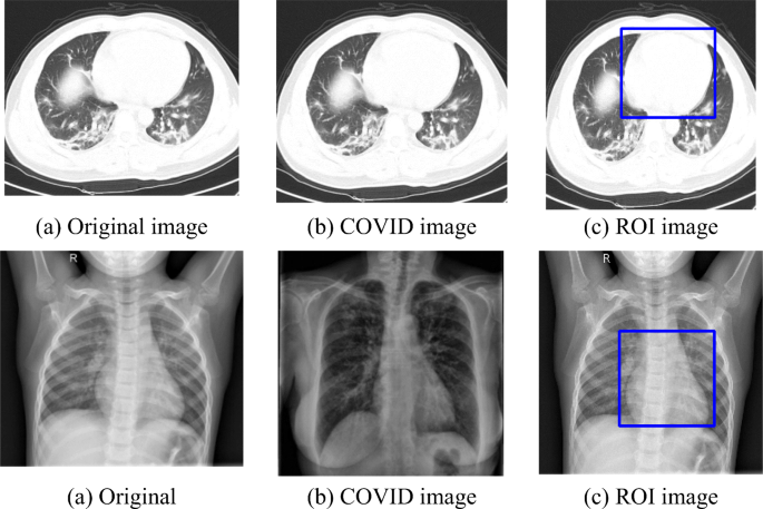

  

  ROI detected images for both CT and X-ray dataset

  Elimination of noise is a significant stage of pre-processing. In this research work, the MMG filter preserves the edges while removing noises from the images present in the datasets. It is used to train the classifier model as well. The quality of denoising has been evaluated using the MSE and PSNR values. Table 8 shows the proposed MSE and PSNR comparison with the existing method. The experimental results show that the proposed MMG filtering technique is more efficient than the other implemented schemes. The proposed approach achieves very fewer MSE values and higher PSNR values, which are the significant characteristics of the best pre-processing technique.

  Table 8 The MSE and PSNR value comparison

• Feature extraction and classification

  In the feature extraction phase, the first-order statistical texture features such as variance, skewness and kurtosis and the second-order statistical texture features such as correlation, entropy, contrast, energy, maximum probability and homogeneity are extracted from the pre-processed images. The Mobile Net model is used for extracting the features from the pre-processed images, and then the modified discrete wavelet approach is used for dimensionality reduction purposes.

  In the classification phase, images were trained and tested to achieve an accurate result. Here, the deep convolutional neural network model i.e. AgileNet (LeNet & AlexNet) and inception-ResNet (GoogLeNet & ResNet) model are used for the COVID-19 diagnosis classification. To solve the overfitting problems in the network, here propose some network optimization schemes, namely, dropout, weight regularization, and batch normalization. Due to the loss function, the performance accuracy of the proposed system got affected, so introduced a novel convolution Aquila neural network to fine-tune the hyperparameters and minimization of the loss function.

4.3.1 COVID-19 detection using DCNN model

• (a) For CT dataset

  The COVID diagnosis can be performed by the new approach of DCNN AgileNet and Inception-ResNet. Here, some network optimization schemes are used to overcome the overfitting issues in the network.

  Figure 8(a) shows the measurement of accuracy level for CT images with various models such as MResNet50, ResNet50, ResNet101, GoogleNet, AlexNet, DenseNet201, VGG16, VGG19, InceptionV3 and Reanet50 + SVM [12] respectively. The achieved accuracy value of the proposed system is 99%, which clearly shows that the proposed model attains more accuracy than the previous models. The performance degradation is due to the maximum complexity of CNN, where many parameters are required to be tuned. Also, a huge amount of training data is needed for the existing DL techniques. But the proposed model uses a minimum number of parameters and provides efficient classification accuracy.

  Fig. 8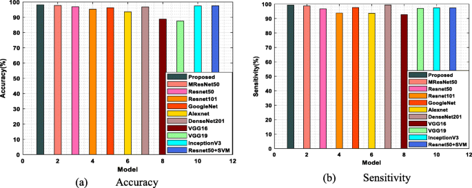

  

  Performance analysis of (a) Accuracy (b) Sensitivity for CT images with various models

  Figure 8(b) mentions the sensitivity levels of the previously implemented model, and the proposed model also clearly proved that the sensitivity level of the proposed model is maximum compared with the existing MResNet50, Reanet50, Reanet101, GoogleNet, AlexNet, DenseNet201, VGG16, VGG19, InceptionV3 and Reanet50 + SVM accordingly. Better classification is not achieved success in the existing techniques because the size of the input images present in the existing algorithm dataset differs. So, it is still a challenging task for the previous algorithms, but the proposed algorithm’s performance is efficient because it deals with very low resolution images. The achieved sensitivity value of the introduced model is 100% and the attained sensitivity levels of existing algorithms are comparatively very low. Table 9 shows the performance measures of the proposed and existing approaches.

  Table 9 Performance analysis of proposed and some of the existing models for CT dataset

  Figure 9 illustrates the performance analysis of specificity and precision for CT images compared with different models, namely, MResNet50, ResNet50, ResNet101, GoogleNet, AlexNet, DenseNet201, VGG16, VGG19, InceptionV3 and ResNet50 + SVM. Figure 9(a) explains the specificity achievements clearly and attains the maximum sensitivity value of 98.5% for the proposed model to the previously implemented approaches. One of the major drawbacks of ResNets is that it is only applicable for deeper networks, so detecting errors in the classification performance was very difficult. Similarly, the learning process becomes inefficient if the network is too shallow. It degrades the sensitivity values of the existing algorithm. Also, dimensionality reduction is not efficiently performed in any previous methods. It increases the computational complexity and also degrades the detection accuracy. But in the proposed algorithm, a discrete wavelet-based approach is used for the dimensionality reduction feature vectors.

  Fig. 9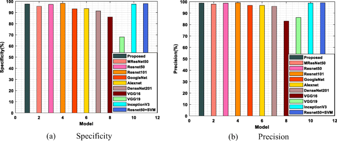

  

  Performance measures of (a) Specificity and (b) Precision for CT images with different models

  Figure 9(b) demonstrates the precision value for CT dataset images with the various existing and proposed models. In that, the different existing models to detect COVID cases are compared with the proposed model to show the effectiveness of the proposed model. The achieved precision value of the proposed model is maximum, i.e. 99.5%, compared with the achievements of the previous work. The specificity and precision metrics of existing algorithms are very low because they do not efficiently use the pooling layers. But in the proposed model, the max polling and mean pooling are utilized to eliminate the overfitting issues and increase the prediction rate.

• (b) For X-ray dataset

  The performance measure, accuracy, is to estimate the proposed model’s effectiveness. Figure 9 illustrates the proposed model accuracy and sensitivity measures for X-ray-dataset. The proposed model accomplishes an increased accuracy rate compared with some existing techniques, namely, MResNet50, ResNet50, ResNet101, GoogleNet, AlexNet, DenseNet201, VGG16, VGG19, InceptionV3 and ResNet50 + SVM [12] shown in Fig. 10(a). The proposed methods attain a maximum accuracy level of 98%, which clearly shows the achieved accuracy value of the proposed is maximum compared to the previous models. The performance degradation of existing models is due to the normalized intensities of chest X-rays are not identified accurately. Also, the existing techniques require many annotation tasks to train the model.

  Fig. 10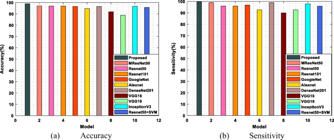

  

  Performance measures of (a) Accuracy and sensitivity for x-ray-dataset with various methods

  Figure 10(b) illustrates the sensitivity values of the proposed and existing approaches for the x-ray dataset. The graph shows the attained sensitivity value of existing methods such as MResNet50, Reanet50, Reanet101, GoogleNet, AlexNet, DenseNet201, VGG16, VGG19, InceptionV3, and Reanet50 + SVM is lower because the dataset quality of the existing methods influences the generalization and robustness of the model. The achieved sensitivity value of the proposed model, i.e. 99%, is maximum because of the best dataset quality.

  Figure 11 illustrates the specificity and precision values for the X-ray dataset and compares the proposed with existing models. The proposed model accomplishes a more specificity rate than the techniques, namely, MResNet50, Reanet50, Reanet101, GoogleNet, AlexNet, DenseNet201, VGG16, VGG19, InceptionV3 and Reanet50 + SVM. Figure 11(a) proves the proposed model achieved an enhanced specificity rate than the previous models. The improved specificity level of the proposed is 98%, and the attained specificity rate of existing techniques MResNet50 is very low. The degradation of specificity and precision rate for the existing techniques is because of the risk prediction factor. The previous VGG-16 model provides only 86% specificity value and 83% precision value as the risk prediction rate for the COVID disease.

  Fig. 11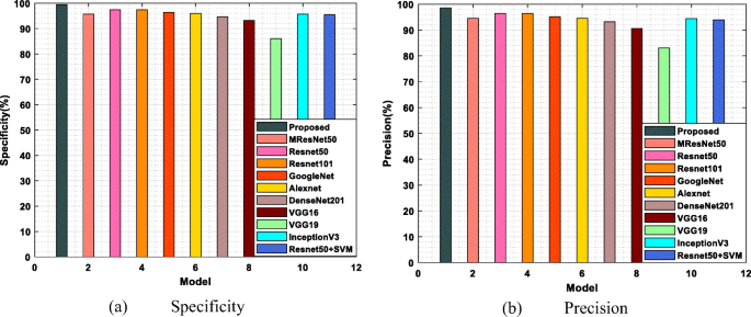

  

  Performance measures of (a) Specificity (b) Precision for X-ray dataset

  Figure 11(b) shows comparatively the achieved precision levels of proposed and existing models. The existing approaches like MResNet50, Reanet50, Reanet101, GoogleNet, AlexNet, DenseNet201, VGG16, VGG19, InceptionV3 and Reanet50 + SVM are compared with the proposed model, and the accomplished precision rate of the proposed model is 97%, which is higher than the previous model. The outcome of existing models is comparatively low because of the rapid increase of noise which is not properly minimized in the pre-processing stage. It leads to a maximum false negative rate, which causes misclassification accuracy. Table 10 tabulates the achieved performance analysis of the proposed and some of the existing models.

  Table 10 Performance analysis of proposed and existing model for X-ray dataset

  The f1-score performance metrics comparison with some existing techniques such as ResNet50, EfficientNetB0, DenseNet121 and mobileNetV2 are given in Tables 9 and 10. The achieved f1-score of the proposed algorithm is maximum compared to other COVID detection algorithms. The training time of the existing techniques is high, which leads to cause degradation in the classification performance. The number of images selected for each case in the proposed model is very few, which highly reduces the training time of the proposed model and produces an efficient f1-score.

• (c) Hybrid analysis of chest X-ray and COVID CT

  Figure 12 shows the classification performance comparison using a hybrid dataset. It is the combination of X-ray and CT datasets. The accuracy, specificity, recall and f1-score values of the proposed method with hybrid chest X-ray and COVID CT dataset are more than the other ResNet50 and EfficientNetB0 [7] with the hybrid dataset.

  Fig. 12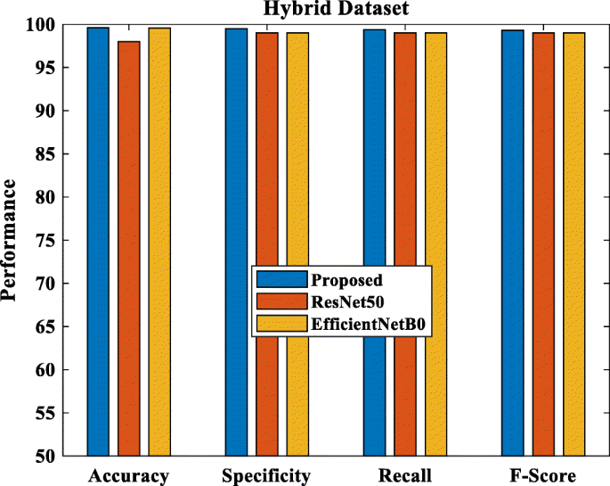

  

  Performance comparison with the hybrid dataset

4.3.2 Confusion matrix analysis

To compare the proposed system’s original value and the predicted value using a confusion matrix for the chest X-ray dataset, testing accuracy and training accuracy are shown, i.e. Figure 13(a) and (b). The classification approach’s predicted accuracy is denoted diagonally for training accuracy. There are 86 COVID cases, 652 Pneumonia cases and 228 normal cases taken into account. From this, 78 samples are correctly classified as COVID-19, and the remaining 8 samples are misclassified. 649 samples are accurately classified as Pneumonia, 3 samples are misclassified, and also 220 samples are correctly classified as normal by using the proposed method, 8 samples get misclassified. It clearly shows that the proposed method’s misclassification level is very low compared to other methods, so it accomplishes better classification accuracy.

Fig. 13

Confusion matrix for chest X-ray dataset

To compare the original value and the predicted value of the proposed system with the aid of a confusion matrix for the COVID CT dataset shown in Fig. 14. The predicted training accuracy of the classification approach is denoted diagonally. There are 245 COVID cases and 325 normal cases taken into account. From this, 242 samples are correctly classified as COVID-19, and the remaining 3 samples are misclassified. 320 samples are accurately classified as normal, and 5 samples are misclassified with the aid of the proposed method. It clearly shows that the proposed method misclassification level is very lower when compared with other methods, so it accomplishes better classification accuracy.

Fig. 14

Confusion matrix for COVID CT dataset

4.3.3 ROC curve for chest X-ray and COVID CT dataset

The receiver operating characteristics (ROC) curve is drawn between true positive rate (TPR) and false negative rate (FNR). Also, it is defined as the trade-off between sensitivity and specificity. The TPR is plotted on the y-axis and FPT on the x-axis. The medical diagnosis system requires a maximum area under the curve (AUC). The trapezoidal approach is used to calculate the AUC by classifying the area into some sections with equal width. By varying the FP rate, the achieved ROC value of the proposed model for normal is 0.9973 and COVID-19 is 0.9977, which clearly shows the proposed model has good indication and provides better classification. Figure 15 illustrates the ROC curve for the chest X-ray dataset.

Fig. 15

ROC curve of chest X-ray dataset

Figure 16 demonstrates the ROC curve for the COVID-CT dataset. The sensitivity (TPR) is plotted on the x-axis, and specificity (FPR) is plotted on the y-axis. The TPR should be higher for the best classification model, keeping FPR as low as possible. If the ROC curve of the introduced model is closest to the top left corner shows superior performance. The obtained ROC curve values for pneumonia are 0.973, for normal cases is 0.986%, and for COVID cases is 1 by changing the FPR rate for the TPR rate.

Fig. 16

ROC curve of CT scan dataset

4.3.4 Accuracy and loss analysis of proposed COVID detection model

In the accuracy curve, the comparison is made with training and validation data for CT and X-ray datasets. According to the graph, our proposed model obtained low or high equalized outcomes in both graphs. When the number of iterations is high, the accuracy is also high. The proposed method is trained for 100 iterations and is highly stable for increased iterations for training and testing the data. In the loss curve, the comparison is made with training and validation data for both CT and X-ray datasets. According to the graph, the loss percentage for the developed method is highly decreased, and if the number of iterations is high, the outcome will be very low. From this graph, can understand that our model is highly stable with increased iterations. Figures 17(a) and (b) show the accuracy and loss curves of the CT and chest X-ray datasets.

Fig. 17

Accuracy and loss curve of the proposed model for CT and X-ray dataset

4.3.5 Five fold cross validation analysis for CT and X-ray dataset

Figure 18 shows the performance measures of the accuracy, sensitivity, specificity and precision values for the proposed and the existing model under different fold counts for the CT dataset. Under flod1, flod2, fold3, fold4 and fold5 the proposed model achieves better for accuracy such as, 99, 98, 98, 97, 97.5, for sensitivity such as, 99.4, 99, 97.9, 97.4, 98.2, for specificity 95, 91.8, 95.6, 94.5, 93.1, for precision 97.6, 96.2, 97.9, 97.3, 96.7 and the achieved accuracy, sensitivity, specificity and precision values for existing MResNet 50 are 98, 96.6, 97.1, 96.5, 96.6; 100, 100, 99, 98, 99; 96, 93, 96, 95, 94; 99, 97, 99, 98, 98 respectively. Comparing the existing model with the proposed model attained a higher performance analysis result than the existing models.

Fig. 18

Performance analysis of accuracy, sensitivity, specificity and precision values for CT dataset under various folds

Figure 19 illustrates the performance analysis of accuracy, sensitivity, specificity and precision for the X-ray dataset under various folds such as fold-1, fold-2, fold-3, fold-4 and fold-5, respectively. The proposed model attains an accuracy of 98%, 97%, 97.2%, 97.4% and 96% under the fold-1, fold-2, fold-3, fold-4 and fold-5 validations. However, the existing model of MResNet50 yields an accuracy of 96.6%, 96.1%, 96.2%, 96.6% and 95.1% under fold-1, fold-2, fold-3, fold-4 and fold-5 validations. And it proves that the proposed model attains a better outcome when compared with the existing MResNet50 model.

Fig. 19

Performance analysis of accuracy, sensitivity, specificity and precision values for X-ray dataset under various folds

For X-ray dataset, the sensitivity of the proposed model is 98.4%, 97.3%, 98.1%, 96.2%, and 98.9% under five cross fold variations. In X-ray dataset, the existing model MResNet50 retains an sensitivity outcome of 99%, 98%, 99%, 97%, and 99.5% under five cross fold variations.

For specificity and precision, the obtained values for the proposed model under various folds such as, fold-1, fold-2, fold-3, fold-4 and fold-5 are 96%, 96.5%, 95.3%, 98%, 93% and 95%, 95.5%, 94.3%, 97, 92.2% respectively. The proposed model achieves maximum values from these values than the previous approaches. Table 11 tabulates the CT and X-ray datasets cross validation for the proposed and existing models.

Table 11 Cross validation results of proposed and existing model on CT and X-ray dataset

4.4 Statistical analysis

The statistical analysis is performed with the Wilcoxon signed-ranked test and computed p-values for all the models. This test is commonly referred to as the non-parametric comparison between two samples. It is implemented to compare two independent samples to carry out a paired variations test of repeated measurements on a single sample. The experimental results, it clearly shows whether its population mean ranks differ or not. The table values conclude that the proposed model achieves better performance than the existing models. If the value of the p value is less than 0.05, the model is considered more efficient than the other, and the outcome is statistically significant. Table 12 demonstrates the Wilcoxon signed-ranked test.

Table 12 Wilcoxon signed-ranked test

5 Discussion

The research work processed in this section is classified into three phases: pre-processing, feature extraction, and classification. The pre-processing phase plays a significant role in the COVID-19 diagnosis. Here, the collected images from the CT and X-ray datasets are pre-processed to eliminate unnecessary noises and enhance the collected images’ quality. By utilizing the MMG hybrid filtering technique, the unwanted noises are get eliminated for further processing. The next is the feature extraction stage, here, the first-order and second-order statistical texture features are extracted from the pre-processed images. The first order statistical textures are skewness, variance and kurtosis. The second-order statistical texture features are GLCM, GLRLM and GLSZM. The modified discrete wavelet-based mobile net model is used to extract the image features. The system’s performance gets degraded because of the maximum dimension of feature vectors. The discrete wavelet-based model is utilized to reduce the dimensionality of the feature vector and achieve more accurate results. The dimensionality reduction is the process of eliminating the minimum contributed features from the images. The presence of these may affect the performance of the proposed model.

Finally, classification stage, here the testing and training are performed on the extracted features based on DCNN. The convolutional Aquila neural network is used to minimize the obtained loss function of the developed model, and the classification of normal and COVID-19 case results are obtained accurately. The accomplished accuracy rate for the proposed model is 99% for the CT dataset and 98% for the X-ray dataset, respectively.

The evaluation results of the proposed model are compared to previous proposed models: MResNet50, Reanet50, Reanet101, GoogleNet, AlexNet, DenseNet201, VGG16 VGG19, InceptionV3 and Reanet50 + SVM models. Furthermore, the previous approaches achieve less performance analysis because of the various disadvantages. The accurate detection of COVID positive and normal cases is very difficult in the DL-based CNN model.

The dropout layer and local response normalization (LRN) layers are used to learn the network better, but in the AlexNet, these two layers are not efficiently used, leading to learning complexity. The VGG architecture consists of very few convolution layers, and each of the layers uses ReLU as the activation function, so the classification accuracy is not satisfactory. In GoogleNet, a separate stack of inception layers are used to improve the detection accuracy. This consequently increases this CNN model and does not completely solve the computational cost and the gradient vanishing issue. The ResNet50 is the most famous CNN model, but the total amount of MACs and weights degrade the detection performance of COVID-19. In DesNet, the outcome of every layer is the input of the next descendant layer this dense connectivity reduces the network parameters, but if any of the layers faces overfitting issue, it will affect the next layer automatically.

In InceptionNet V3, the proper usage of residual connections in Xception structure will cause accelerated convergence and excellent detection performance at the final. Still, it is failed to be used appropriately in this existing CNN model. The reduction blocks introduced in this module enhance the training speed, but a robust connection was required unless it makes the network learning process more complex. In the existing CapsNet, the COVID is present in the given region and is examined correctly. Still, there is a huge overlapping between the two classes available in this CNN model. These all are the issues that motivate us to design an efficient deep CNN model. The major layers exploited in this proposed architecture are depthwise separable convolution. It highly reduces the computational cost and achieves maximum training speed. The major benefit of using this model is fewer parameter usage it leads to achieving faster running time and classification outcomes. The number of images used for the COVID-19 patients is less in the existing VGG16, denseNet121, xception, NASnet, efficient net, and its minimum accuracy levels are 79.01%, 89.96%, 88.03%, 85.03% and 93.48% respectively.

Further, the CNN classification model for medical images based on different edges in a neural network achieves an accuracy level is 85%; this system classifies the images by performing the pre-processing step. It affects the accuracy level of this classification model system. In the deep LSTM model, the enormous memory bandwidth usage in the real-time application degrades the training and testing model accuracy, i.e. 80% and 20%.

Compared with the above mentioned existing methods, our proposed model achieves more accurate results in accuracy, precision, specificity and sensitivity performance measures for the dataset X-ray and CT. Our proposed approach uses a convolution Aquila neural network to fine-tune the hyperparameters and loss function minimization. Then utilize the efficient modified discrete wavelet based Mobile Net model for feature extraction and wavelet approach for dimensionality reduction. The performance metrics prove the efficiency of our proposed model. The performance can be analyzed and compared with the previously implemented models by varying folds. The previous optimization methods are not strong and may cause an imbalance in the exploitation and exploration schemes. But the Aquila optimizer provides better exploitation and exploration results. Furthermore, it attains a more flexible outcome with fine-tune parameters. The Aquila optimizer and the proposed network model for loss function reduction are normalised.

6 Conclusion and future scope

This research work introduces a novel deep learning technique for detecting the COVID-19 disease based on a DCNN. For medical specialists, detection of COVID-19 cases is a difficult task. The chest X-ray and CT plays a significant role in the COVID-19 diagnosis. Our proposed method consists of pre-processing, feature extraction, and classification stages. In the pre-processing stage, the irrelevant noises are removed from the raw images gathered from the X-ray and CT datasets. By using the MMG hybrid filtering approach, the unwanted noises are removed and enhance the quality of the images too. The next step is feature extraction, in this stage, the features are extracted based on first and second order statistical texture features.

Here, a modified Mobile Net model effectively reduces the dimensionality wavelet approach. The final stage is the classification, here, a convolutional Aquila covid detection NN is modeled to classify the normal and COVID-19 cases accurately. By using the Aquila optimizer, the loss function gets reduced. Our proposed approach achieves better accuracy for COVID-19 detection. The performance metrics such as specificity, accuracy, precision and sensitivity are analyzed for the proposed method. The obtained specificity, accuracy, precision and sensitivity values for CT dataset are: 100%, 99%, 99.5%, 98.5% and the appropriate values for X-ray dataset are: 98%, 99%, 98% and 97% accordingly. Various parameters can also be conducted in future based on deep learning techniques for better diagnosis of COVID-19. The defined model plays a major role in COVID classification; however, the defined model lacks due to some limitations, such as the inclusion of the bionic model. The Aquila model attains a local minimum due to its high dimensionality if the hidden units increase. This will corrupt the detection performance of the proposed model. Deep learning (DL) has high potential and can be utilized to mitigate and combat the spread of the COVID-19 pandemic significantly. Besides several benefits and positive results, various limitations and challenges associated with the DL implementation must be evaluated and addressed. The ultrasound scans and magnetic resonance imaging (MRI) show excellent classification results than the X-ray and CT images. Hence, for the COVID-19 classification, these schemes must be considered in the future to train the models.

References

Abd Elaziz M, Dahou A, Alsaleh NA, Elsheikh AH, Saba AI, Ahmadein M (2021) Boosting COVID-19 image classification using MobileNetV3 and aquila optimizer algorithm. Entropy 23(11):1383
Abualigah L, Yousri D, Elaziz MA, Ewees AA, Al-Qaness MAA, Gandomi AH (2021) Aquila optimizer: a novel meta-heuristic optimization algorithm. Comput Ind Eng 157:107250
Ahsan M, Based MA, Haider J, Kowalski M (2021) COVID-19 detection from chest X-ray images using feature fusion and deep learning. Sensors 21(4):1480
Akter S, Shamrat FMJM, Chakraborty S, Karim A, Azam S (2021) COVID-19 detection using deep learning algorithm on chest X-ray images. Biology 10(11):1174
Cabello F, León J, Iano Y, Arthur R (2015) Implementation of a fixed-point 2D Gaussian Filter for Image Processing based on FPGA. In 2015 Signal processing: algorithms, architectures, arrangements, and applications (SPA), IEEE 28–33
Chen JIZ (2021) Design of accurate classification of COVID-19 disease in X-ray images using deep learning approach. J ISMAC 3(02):132–148
Chola C, Mallikarjuna P, Muaad AY, Benifa JVB, Hanumanthappa J, Al-antari MA (2021) A hybrid deep learning approach for COVID-19 diagnosis via CT and X-ray medical images. Comput Sci Math Forum, MDPI 2(1):13
de Oliveira HM, Ospina R, Leiva V, Martin-Barreiro C, Chesneau C (2022) A new wavelet-Based privatization mechanism for probability distributions. Sensors 22(10):3743
Demir F (2021) DeepCoroNet: a deep LSTM approach for automated detection of COVID-19 cases from chest X-ray images. Appl Soft Comput 103:107160
El-Kenawy E-SM, Mirjalili S, Ibrahim A, Alrahmawy M, El-Said M, Zaki RM, Eid MM (2021) Advanced meta-heuristics, convolutional neural networks, and feature selectors for efficient COVID-19 X-ray chest image classification. IEEE Access 9:36019–36037
Elmuogy S, Hikal NA, Hassan E (2021) An efficient technique for CT scan images classification of COVID-19. J Intell Fuzzy Syst 40(3):5225–5238
Elpeltagy M, Sallam H (2021) Automatic prediction of COVID− 19 from chest images using modified ResNet50. Multimed Tools Appl 80(17):26451–26463
Garg G, Juneja M (2018) A survey of prostate segmentation techniques in different imaging modalities. Curr Med Imaging 14(1):19–46
Garg G, Juneja M (2018) Cancer detection with prostate zonal segmentation—a review. In: Proceedings of the international conference on computing and communication systems, springer, Singapore 829-835
Garg G, Juneja M (2018) A survey on computer-aided detection techniques of prostate Cancer. In: Progress in advanced computing and intelligent engineering, springer, Singapore 115-125
Garg G, Juneja M (2019) A survey of denoising techniques for multi-parametric prostate MRI. Multimed Tools Appl 78(10):12689–12722
Garg G, Juneja M (2021) Particle swarm optimization based segmentation of Cancer in multi-parametric prostate MRI. Multimed Tools Appl 80(20):30557–30580
Goyal M, Tewatia N, Vashisht H, Jain R, Kumar S (2021) Novel corona virus (COVID-19); global efforts and effective investigational medicines: a review. J Infect Public Health 14(7):910–921
Guptha NS, Patil KK (2017) Earth mover's distance-based CBIR using adaptive regularised kernel fuzzy C-means method of liver cirrhosis histopathological segmentation, Published Online June 21. 39–46
Guptha NS, Patil KK (2018) Detection of macro and micro nodule using online region based-active contour model in histopathological liver cirrhosis. Int J Intell Eng Syst 11(2):256–265
Hemalatha G, Sumathi CP (2016) Preprocessing techniques of facial image with median and Gabor filters. In: 2016 international conference on information communication and embedded systems (ICICES), IEEE 1-6
Houssein EH, Emam MM, Ali AA (2021) Improved manta ray foraging optimization for multi-level thresholding using COVID-19 CT images. Neural Comput & Applic 33(24):16899–16919
Huang M-L, Liao Y-C (2022) A lightweight CNN-based network on COVID-19 detection using X-ray and CT images. Comput Biol Med 146:105604
Huang S, Yang J, Fong S, Zhao Q (2021) Artificial intelligence in the diagnosis of COVID-19: challenges and perspectives. Int J Biol Sci 17(6):1581–1587
Hussein AF, ArunKumar N, Ramirez-Gonzalez G, Abdulhay E, Tavares JMRS, de Albuquerque VHC (2018) A medical records managing and securing blockchain based system supported by a genetic algorithm and discrete wavelet transform. Cogn Syst Res 52:1–11
Ismael MR, Abdel-Qader I (2018) Brain tumor classification via statistical features and back-propagation neural network. In: 2018 IEEE international conference on electro/information technology (EIT), 0252-0257
Iyer TJ, Raj ANJ, Ghildiyal S, Nersisson R (2021) Performance analysis of lightweight CNN models to segment infectious lung tissues of COVID-19 cases from tomographic images. PeerJ Computer Science 7:e368
Jamil S, Rahman M, Haider A (2021) Bag of features (BoF) Based deep learning framework for bleached corals detection. Big Data Cogn Comput 5(4):53
Kumar A, Sodhi SS (2020) Comparative analysis of gaussian filter, median filter and denoise autoenocoder. In: 2020 7th international conference on computing for sustainable global development (INDIACom), IEEE 45-51
Kumar M, Shakya D, Kurup V, Suksatan W (2022) COVID-19 prediction through X-ray images using transfer learning-based hybrid deep learning approach. Mater Today: Proc 51:2520–2524
Maheshan CM, Kumar HP (2020) Performance of image pre-processing filters for noise removal in transformer oil images at different temperatures. SN Appl Sci 2(1):1–7
Nigam B, Nigam A, Jain R, Dodia S, Arora N, Annappa B (2021) COVID-19: automatic detection from X-ray images by utilizing deep learning methods. Expert Syst Appl 176:114883
Pontone G, Scafuri S, Mancini ME, Agalbato C, Guglielmo M, Baggiano A, Muscogiuri G, Fusini L, Andreini D, Mushtaq S, Conte E, Annoni A, Formenti A, Gennari AG, Guaricci AI, Rabbat MR, Pompilio G, Pepi M, Rossi A (2021) Role of computed tomography in COVID-19. J Cardiovasc Comput Tomogr 15(1):27–36
Prashant Patel, (n.d.) Chest X-ray (Covid-19 & Pneumonia), Accessed at: https://www.kaggle.com/prashant268/chest-xray-covid19-pneumonia
Praveena HD, Guptha NS, Kazemzadeh A, Parameshachari BD, Hemalatha KL (2022) Effective CBMIR System Using Hybrid Features-Based Independent Condensed Nearest Neighbor Model. J Healthc Eng 2022:3297316
Rahman T, Khandakar A, Qiblawey Y, Tahir A, Kiranyaz S, Kashem SBA, Chowdhury ME (2021) Exploring the effect of image enhancement techniques on COVID-19 detection using chest X-ray images. Comput Biol Med 132:104319
Salehi M, Mohammadi R, Ghaffari H, Sadighi N, Reiazi R (2021) Automated detection of pneumonia cases using deep transfer learning with paediatric chest X-ray images. Br J Radiol 94(1121):20201263
Shankar K, Perumal E, Díaz VG, Tiwari P, Gupta D, Saudagar AKJ, Muhammad K (2021) An optimal cascaded recurrent neural network for intelligent COVID-19 detection using chest X-ray images. Appl Soft Comput 113:107878
Shankar K, Mohanty SN, Yadav K, Gopalakrishnan T, Elmisery AM (2021) Automated COVID-19 diagnosis and classification using convolutional neural network with fusion based feature extraction model. Cogn Neurodyn:1–14. https://doi.org/10.1007/s11571-021-09712-y
Shankar K, Perumal E, Tiwari P, Shorfuzzaman M, Gupta D (2021) Deep learning and evolutionary intelligence with fusion-based feature extraction for detection of COVID-19 from chest X-ray images. Multimed Syst:1–13
Siddiqui SY, Abbas S, Khan MA, Naseer I, Masood T, Khan KM, Almotiri SH (2021) Intelligent decision support system for COVID-19 empowered with deep learning. Comput., mater. Continua 66(2):1719–1732
Thamer SA, Alshmmri MA (2022) A review of machine learning and deep learning approaches for COVID-19 diagnosis. Int J Mech Eng 7(1):6523–6534
Tuncer T, Ozyurt F, Dogan S, Subasi A (2021) A novel Covid-19 and pneumonia classification method based on F-transform. Chemom Intell Lab Syst 210:104256
Zhao J, Zhang Y, He X, Xie P (2020) Covid-ct-dataset: a ct scan dataset about covid-19. arXiv preprint arXiv:2003.13865 490
Funding
No funding is provided for the preparation of manuscript.
Author information
Authors and Affiliations
Contributions
All authors have equal contributions in this work.
Corresponding author
Ethics declarations
Ethical approval
This article does not contain any studies with human participants or animals performed by any of the authors.
Consent to participate
All the authors involved have agreed to participate in this submitted article.
Consent to publish
All the authors involved in this manuscript give full consent for publication of this submitted article.
Conflict of interest
Authors declare that they have no conflict of interest.
Additional information
Publisher’s note
Springer Nature remains neutral with regard to jurisdictional claims in published maps and institutional affiliations.
Rights and permissions
Springer Nature or its licensor (e.g. a society or other partner) holds exclusive rights to this article under a publishing agreement with the author(s) or other rightsholder(s); author self-archiving of the accepted manuscript version of this article is solely governed by the terms of such publishing agreement and applicable law.
About this article
Cite this article
Tallapragada, V.S., Manga, N.A. & Kumar, G.P. A novel COVID diagnosis and feature extraction based on discrete wavelet model and classification using X-ray and CT images. Multimed Tools Appl 82, 26183–26224 (2023). https://doi.org/10.1007/s11042-023-14367-4
Received:
Revised:
Accepted:
Published:
Issue Date:
DOI: https://doi.org/10.1007/s11042-023-14367-4