
Abstract
We show how to construct, by exploiting adiabatic time and length scale separation between atomistic and continuum mechanics, a multiscale scheme for continuum dynamics free from macroscopic constitutive modeling. To do so, we introduce a new set of degrees of freedom that simultaneously represent the macroscopic and the microscopic dynamics, based on a space tessellation. In this new formulation, the dynamics of the macroscopic fields steers the microscopic particle dynamics by producing the conditions under which they evolve and, concurrently, the particle dynamics drives the evolution of the macroscopic fields by providing them with atomistically based constitutive information. Under conditions of adiabatic separation both in time and length scales, it is possible to decimate the tessellating cells and let the macroscopic equations of motion be driven by the time average of the terms coupling them with the microscopic degrees of freedom.
Notes
We use \(\,\approx \,,\,\gtrapprox \,,\,\lessapprox \,\) to denote, respectively, the relations ‘is of the same order of magnitude of,’ ‘is at least of the order of magnitude of,’ and ‘is at most of the order of magnitude of.’
The inner/outer diameter of a cell is the sup/inf of the diameters of inscribed/circumscribed balls. The inner/outer diameter of a face is the sup/inf of the diameters of inscribed/circumscribed disks.
We define the tensor multiplication \(\otimes \) as the one for which the tensor product of two vectors \(\varvec{a}\), \(\varvec{b}\) acts on all vector \(\varvec{u}\) as follows: \((\varvec{a}\!\otimes \!\varvec{b})\varvec{u}=(\varvec{a}\!\cdot \!\varvec{u})\varvec{b}\), where the dot denotes the inner product between vectors. In Cartesian index notation: \((\varvec{a}\!\otimes \!\varvec{b})_{\alpha \beta }=a_{\beta }b_{\alpha }\), since \(((\varvec{a}\!\otimes \!\varvec{b})\varvec{u})_{\alpha }\!=a_{\beta }u_{\beta }\,b_{\alpha }\) (sum over repeated indices). In this context, \((\varvec{a}\!\otimes \!\varvec{b})^{\!\top }\!\!=\varvec{b}\!\otimes \!\varvec{a}\). For all tensor \(\varvec{L}\), \((\varvec{L}\varvec{a})\!\cdot \!\varvec{b}=\varvec{L}\!\cdot \!(\varvec{a}\!\otimes \!\varvec{b})\), where the dot on the left-hand side denotes the inner product between vectors, while the dot on the right-hand side denotes the inner product between tensors, defined as: \(\varvec{L}\!\cdot \!\varvec{M}\,\,{:=}\,\,\textrm{tr}(\varvec{L}^{\!\top }\!\varvec{M})\) for all tensors \(\varvec{L},\varvec{M}\), with tr the trace and \(\varvec{L}^{\!\top }\!\;\)the transpose of \(\varvec{L}\). In Cartesian index notation: \(\varvec{L}\!\cdot \!\varvec{M}\!=\!L_{\alpha \beta }M_{\alpha \beta }\), and \((\varvec{L}\varvec{a})\!\cdot \!\varvec{b}=L_{\alpha \beta }a_{\beta }b_{\alpha }\). These definitions imply \(\,\varvec{a}\!\otimes \!(\varvec{L}\varvec{b})=\varvec{L}(\varvec{a}\!\otimes \!\varvec{b})\), and \(\,(\varvec{L}\varvec{a})\!\otimes \!\varvec{b}=(\varvec{a}\!\otimes \!\varvec{b})\varvec{L}^{\!\top }\!\).
The Euler tensor \(\varvec{E}\) and the widely used inertia tensor \(\varvec{J}\) are related as follows: \(\varvec{J}=(\textrm{tr}\varvec{E})\varvec{I}-\varvec{E}\).
Via the rules \((\varvec{L}\varvec{a})\!\cdot \!\varvec{b}=\varvec{L}\!\cdot \!(\varvec{a}\!\otimes \!\varvec{b})\) and \(\varvec{a}\!\otimes \!(\varvec{L}\varvec{b})=\varvec{L}(\varvec{a}\!\otimes \!\varvec{b}):\;\)see footnote 3.
We use \(\equiv \) to denote equivalence of symbols.
In Cartesian index notation, \(\textrm{L}_{\alpha \beta }\!=\textrm{v}_{\alpha ,\beta }\), where a subscript comma denotes partial derivative.
Since \(\varvec{\chi }_{\tau }\) is invertible, \(\varvec{\chi }_{\tau }(\varvec{y})\ne \varvec{\chi }_{\tau }(\varvec{x})\) for all \(\varvec{y}\ne \varvec{x}\). Then, letting \(\varvec{u}\,\,{:=}\,\,\varvec{y}\!-\!\varvec{x}\ne \varvec{0}\) tend to \(\varvec{0}\), one has that \(\varvec{\chi }_{\tau }(\varvec{x}+\varvec{u})-\varvec{\chi }_{\tau }(\varvec{x})\rightarrow {\textbf {F}}_{\tau }(\varvec{x})\varvec{u}\ne \varvec{0}\), i. e., the tensor \({\textbf {F}}_{\tau }(\varvec{x})\) maps nonzero vectors to nonzero vectors and is hence invertible.
Equality (2.43) is often written in the form

leaving out the essential detail that the gradient of \(\varvec{\chi }_{\tau }\) is taken with respect to the initial marker position, while the gradient of \(\textbf{v}_{\tau }\) is taken with respect to the current position of the same marker. This loss of information is somehow compensated by denoting the gradient operator \(\nabla \) by ‘Grad’ or ‘grad,’ depending of whether it is applied in the initial or in the current configuration. This way of writing (2.43) leaves implicit that, if \(\textrm{Grad}\varvec{\chi }_{\tau }\) is evaluated at \(\varvec{x}\), then \(\textrm{grad}\textbf{v}_{\tau }\) should be evaluated in \(\varvec{\xi }\!=\!\varvec{\chi }(\varvec{x},\tau )\).
Recall from Sect. 2.2.1 that cells are open convex polyhedra.
To prove this, consider a mesoscopic cell
 , and let
\(\varvec{n}\) be the unit outward normal to one of its faces, say
, and let
\(\varvec{n}\) be the unit outward normal to one of its faces, say
 . Then, construct the cell
 by moving
 to
to
 and extending the adjoining faces accordingly. Construct the cell
 analogously, moving
 to
to
 . For all sufficiently small
\(\varepsilon \!>0\),
. For all sufficiently small
\(\varepsilon \!>0\),
 and
and
 are mesoscopic cells. Applying (2.34)
\(_1\) to each of them yields the two equalities
are mesoscopic cells. Applying (2.34)
\(_1\) to each of them yields the two equalities
 and
and
 . Combining them with the identity
 , where
\(\sqcup \) denotes disjoint union, yields
, where
\(\sqcup \) denotes disjoint union, yields

Since
 for all
\(\varepsilon \!>\!0\), this proves that the net mass flux due to thermal velocities through
for all
\(\varepsilon \!>\!0\), this proves that the net mass flux due to thermal velocities through
 is mesoscopically negligible.
If the k-th cell lies on the periphery of
 , the force
\(\textbf{f}_i^{\ne k}\)(
\(\tau \)) includes the force exerted by the confining field, which we suppose to have nonnegligible effects only in a thin boundary layer of
, the force
\(\textbf{f}_i^{\ne k}\)(
\(\tau \)) includes the force exerted by the confining field, which we suppose to have nonnegligible effects only in a thin boundary layer of
 .
.In fact, \(\textbf{m}^h\!=-{\textstyle \frac{1}{2}}\varvec{\varepsilon }\varvec{M}^h\), with \(\varvec{\varepsilon }\) the alternating pseudo-tensor. In Cartesian index notation: \(\textrm{m}^h_{\alpha }\!\!=\!-{\textstyle \frac{1}{2}}\varepsilon _{\alpha \beta \gamma }M^h_{\beta \gamma }.\)
The square roots of the eigenvalues of \(\varvec{G}^{h}_0\) are the principal gyration radii of
 , all of which are
\(\approx L_{\mathsf m}\).
, all of which are
\(\approx L_{\mathsf m}\).See Appendix 4 for definitions and relevant properties of running time averages.
The equalities \((\varvec{L}\varvec{a})\!\cdot \!\varvec{b}=\varvec{a}\!\cdot \!(\varvec{L}^{\!\top }\varvec{b})= \varvec{L}\!\cdot \!(\varvec{a}\!\otimes \!\varvec{b})\) are used here: see footnote 3.
The rules \((\varvec{L}\varvec{a})\!\cdot \!\varvec{b}=\varvec{L}\!\cdot \!(\varvec{a}\!\otimes \!\varvec{b})\), \(\varvec{a}\!\otimes \!(\varvec{L}\varvec{b})=\varvec{L}(\varvec{a}\!\otimes \!\varvec{b})\), and \((\varvec{a}\!\otimes \!\varvec{b})^{\!\top }\!\!=\varvec{b}\!\otimes \!\varvec{a}\) (see footnote 3) are used here and below.
The rule \((\varvec{L}\varvec{a})\!\cdot \!\varvec{b}=\varvec{L}\!\cdot \!(\varvec{a}\!\otimes \!\varvec{b})\) (see footnote 3) is applied here.
By this we mean that \(\varvec{y}\) is the center of area of the face
 .
.The field \(\textbf{n}^h_{\tau }\) needs to be defined only almost-everywhere with respect to the area measure. On the boundary of a polyhedron, the unit normal field is not defined on edges and vertices—which have zero area, and hence do not contribute to the integrals in (D5)—and is piecewise constant elsewhere.
In Cartesian index notation, the divergence of \(\textbf{T}\) is represented by \((\text {div}\textbf{T})_\alpha \!=\textrm{T}_{\alpha \beta ,\beta }\). Equivalently, \(\text {div}(\textbf{T}^{\top }\!\textbf{v})\!=\) \((\text {div}\textbf{T})\!\cdot \!\textbf{v}+\textbf{T}\!\cdot \!\nabla \textbf{v}\) for all vector field \(\textbf{v}\). In fact, in Cartesian index notation, \((\textrm{T}_{\alpha \beta }\textrm{v}_{\alpha })_{,\beta }=\textrm{T}_{\alpha \beta ,\beta }\textrm{v}_{\alpha }+\textrm{T}_{\alpha \beta }\textrm{v}_{\alpha ,\beta }. \)
It can be shown [1] that the Piola stress as defined in (D13) is the field that, for all oriented mesoscopic face
 , satisfies the equality (cf. (D8) for notations)

where \(\varvec{y}\) is the center of
 and the unit vectors
\(\varvec{n}\) and
\(\varvec{n}_{_0}\) are normal, respectively, to
and the unit vectors
\(\varvec{n}\) and
\(\varvec{n}_{_0}\) are normal, respectively, to
 and its parent face
 . Equality (*) implies that
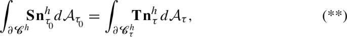
where \(\textbf{n}^h_{\tau }\) and \(\textbf{n}^h_{\tau _{_{0}}}\) denote the unit outer normal fields on
 and
and
 , respectively. Applying the divergence theorem and the change of variable theorem to (**) yields equality (D14).

 , and let
 . Then, construct the cell
 by moving
 to
to
 and extending the adjoining faces accordingly. Construct the cell
 analogously, moving
 to
to
 . For all sufficiently small
 and
and
 are mesoscopic cells. Applying (
 and
and
 . Combining them with the identity
 , where

 for all
 is mesoscopically negligible.
 , the force
 .
. , all of which are
 .
. , satisfies the equality (cf. (
 and the unit vectors
 and its parent face
 . Equality (*) implies that

 and
and
 , respectively. Applying the divergence theorem and the change of variable theorem to (**) yields equality (
References
Gurtin, M.E., Fried, E., Anand, L.: The Mechanics and Thermodynamics of Continua. Cambridge University Press, Cambridge (2010). https://doi.org/10.1017/CBO9780511762956
Parrinello, M., Rahman, A.: Crystal structure and pair potentials: a molecular-dynamics study. Phys. Rev. Lett. 45, 1196–1199 (1980). https://doi.org/10.1103/PhysRevLett.45.1196
Parrinello, M., Rahman, A.: Polymorphic transitions in single crystals: a new molecular dynamics method. J. Appl. Phys. 52(12), 7182–7190 (1981). https://doi.org/10.1063/1.328693
Andersen, H.C.: Molecular dynamics simulations at constant pressure and/or temperature. J. Chem. Phys. 72(4), 2384–2393 (1980). https://doi.org/10.1063/1.439486
Ray, J.R., Rahman, A.: Statistical ensembles and molecular dynamics studies of anisotropic solids. J. Chem. Phys. 80(9), 4423–4428 (1984). https://doi.org/10.1063/1.447221
Ribarsky, M.W., Landman, U.: Dynamical simulations of stress, strain, and finite deformations. Phys. Rev. B 38, 9522–9537 (1988). https://doi.org/10.1103/PhysRevB.38.9522
Murdoch, A.I.: The motivation of continuum concepts and relations from discrete considerations. Q. J. Mech. Appl. Math. 36(2), 163–187 (1983). https://doi.org/10.1093/qjmam/36.2.163
Murdoch, A.I.: A corpuscular approach to continuum mechanics: basic considerations. Arch. Ration. Mech. Anal. 88(4), 291–321 (1985). https://doi.org/10.1007/BF00250868
Murdoch, A.I., Bedeaux, D.: Continuum equations of balance via weighted averages of microscopic quantities. Proceedings of the Royal Society of London. Series A: Mathematical and Physical Sciences 445(1923), 157–179 (1994). https://doi.org/10.1098/rspa.1994.0054
Hardy, R.J.: Formulas for determining local properties in molecular-dynamics simulations: shock waves. J. Chem. Phys. 76(1), 622–628 (1982). https://doi.org/10.1063/1.442714
Podio-Guidugli, P.: On (Andersen-)Parrinello-Rahman molecular dynamics, the related metadynamics, and the use of the Cauchy-Born rule. J. Elast. 100(1), 145–153 (2010). https://doi.org/10.1007/s10659-010-9250-0
DiCarlo, A.: A major serendipitous contribution to continuum mechanics. Mech. Res. Commun. 93, 41–46 (2018). https://doi.org/10.1016/j.mechrescom.2017.10.002
DiCarlo, A.: Continuum mechanics as a computable coarse-grained picture of molecular dynamics. J. Elast. 135(1), 183–235 (2019). https://doi.org/10.1007/s10659-019-09734-y
DiCarlo, A., Podio-Guidugli, P.: From point particles to body points. Math. Eng. 4(1), 1–29 (2022). https://doi.org/10.3934/mine.2022007
Goldstein, H.: Classical Mechanics, 2nd edn. Addison-Wesley, Reading, MA (1980)
Tadmor, E.B., Miller, R.E.: Modelling Materials: Continuum, Atomistic and Multiscale Techniques. Cambridge University Press, Cambridge (2011). https://doi.org/10.1017/CBO9780511762956
Volosov, V.M.: Averaging in systems of ordinary differential equations. Russ. Math. Surv. 17(6), 1–126 (1962). https://doi.org/10.1070/RM1962v017n06ABEH001130
Caswell, R.S., Danos, M.: On the accuracy of the adiabatic separation method. J. Math. Phys. 11(2), 349–354 (1970). https://doi.org/10.1063/1.1665147
Papanicolaou, G.C.: Some probabilistic problems and methods in singular perturbations. Rocky Mt. J. Math. 6(4), 653–674 (1976). https://doi.org/10.1216/RMJ-1976-6-4-653
Pavliotis, G.A., Stuart, A.M.: Multiscale Methods: Averaging and Homogenization. Springer, New York, NY (2008). https://doi.org/10.1007/978-0-387-73829-1
Kevrekidis, I.G., Gear, C.W., et al.: Equation-free, coarse-grained multiscale computation: enabling microscopic simulators to perform system-level analysis. Commun. Math. Sci. 4(1), 715–762 (2003). https://doi.org/10.4310/CMS.2003.v1.n4.a5
Gear, C.W., Li, J., Kevrekidis, I.G.: The gap-tooth method in particle simulations. Phys. Lett. A 316(3), 190–195 (2003). https://doi.org/10.1016/j.physleta.2003.07.004
Kevrekidis, I.G., Samaey, G.: Equation-free multiscale computation: algorithms and applications. Annu. Rev. Phys. Chem. 60(1), 321–344 (2009). https://doi.org/10.1146/annurev.physchem.59.032607.093610
Irving, J.H., Kirkwood, J.G.: The statistical mechanical theory of transport processes. IV. The equations of hydrodynamics. J. Chem. Phys. 18(6), 817–829 (1950). https://doi.org/10.1063/1.1747782
Capecchi, D., Ruta, G., Trovalusci, P.: From classical to Voigt’s molecular models in elasticity. Arch. Hist. Exact Sci. 64(5), 525–559 (2010). https://doi.org/10.1007/s00407-010-0065-y
Born, M., Huang, K.: Dynamical Theory of Crystal Lattices, 1st edn. Clarendon Press, Oxford (1954)
Squire, D.R., Holt, A.C., Hoover, W.G.: Isothermal elastic constants for argon. Theory and Monte Carlo calculations. Physica 42(3), 388–397 (1969). https://doi.org/10.1016/0031-8914(69)90031-7
Hoover, W.G., Holt, A.C., Squire, D.R.: Adiabatic elastic constants for argon. Theory and Monte Carlo calculations. Physica 44(3), 437–443 (1969). https://doi.org/10.1016/0031-8914(69)90217-1
Ericksen, J.L.: On the Cauchy-Born rule. Math. Mech. Solids 13(3–4), 199–220 (2008). https://doi.org/10.1177/1081286507086898
Verlet, L.: Computer “experiments’’ on classical fluids. I. Thermodynamical properties of Lennard-Jones molecules. Phys. Rev. 159, 98–103 (1967). https://doi.org/10.1103/PhysRev.159.98
Swope, W.C., Andersen, H.C., Berens, P.H., Wilson, K.R.: A computer simulation method for the calculation of equilibrium constants for the formation of physical clusters of molecules: application to small water clusters. J. Chem. Phys. 76(1), 637–649 (1982). https://doi.org/10.1063/1.442716
Ryckaert, J.-P., Ciccotti, G., Berendsen, H.J.C.: Numerical integration of the Cartesian equations of motion of a system with constraints: molecular dynamics of n-alkanes. J. Comput. Phys. 23(3), 327–341 (1977). https://doi.org/10.1016/0021-9991(77)90098-5
Ciccotti, G., Ryckaert, J.P.: Molecular dynamics simulation of rigid molecules. Comput. Phys. Rep. 4(6), 346–392 (1986). https://doi.org/10.1016/0167-7977(86)90022-5
Andersen, H.C.: Rattle: a “velocity" version of the shake algorithm for molecular dynamics calculations. J. Comput. Phys. 52(1), 24–34 (1983). https://doi.org/10.1016/0021-9991(83)90014-1
Acknowledgements
We are grateful to CECAM for organizing the 2016 workshop “Marrying continuum and molecular physics: the Andersen-Parrinello-Rahman method revised into a scale bridging device,” that laid the basis of the long-term research project underlying the present paper. In that occasion, as in many others before and after—in particular, at the Spring Course “Hierarchical multiscale methods using the Andersen-Parrinello-Rahman formulation of molecular dynamics,” generously hosted in April 2017 by Eliot Fried at OIST—we profited from discussions with Paolo Podio-Guidugli, whom we gratefully thank for his contribution. We wish to thank all reviewers, whose keen criticisms and constructive suggestions greatly helped us to deepen and streamline our arguments and to make this paper more readable.
Author information
Authors and Affiliations
Corresponding author
Ethics declarations
Conflicts of interest
On behalf of all authors, the corresponding author states that there is no conflict of interest.
Additional information
Publisher's Note
Springer Nature remains neutral with regard to jurisdictional claims in published maps and institutional affiliations.
This article belongs to the themed collection: Mathematical Physics and Numerical Simulation of Many-Particle Systems; V. Bach and L. Delle Site (eds.).
Appendices
Appendix A List of selected notations
Pointers between square brackets refer to where each symbol is defined or first used.
- \(\approx \):
-
is of the same order of magnitude of [note 1]
- \(\gtrapprox \):
-
is at least of the order of magnitude of [note 1]
- \(\lessapprox \):
-
is at most of the order of magnitude of [note 1]
- \(\cong \):
-
equal to within a preset mesoscopic tolerance [(2.27)]
- \(\equiv \):
-
equivalence of symbols [note 6]
 :
:-
local streaming field at cell
 [(2.13)]
 - \(\kappa _i\):
-
locator index of the i-th particle [(2.64)]
- \(\varvec{\lambda }^{\!k}\), \(\varvec{\Lambda }^{\!k}\):
-
Lagrange multipliers affecting particles in the k-th cell [(3.9)]
 :
:-
mass coefficient of the i-th particle in cell
 [(2.8)]
 - \(\mu _i^k\):
-
mass coefficient of the i-th particle in the k-th moving cell [(2.79)]
 :
:-
volume-averaged mass of particles currently in
 [(2.35)]
 - \(\varrho \):
-
macroscopic mass density field [(2.37)]
 :
:-
presence index of the i-th particle in cell
 [(2.9)]
 - \(\varphi _i^{k}\):
-
presence index of the i-th particle in the k-th moving cell [(2.63)]
- \(\varvec{\chi }\):
-
macroscopic (marker) motion [(2.41)]
 :
:-
moving mesoscopic cell initially centered at \(\varvec{x}\) [(2.45)]
 :
:-
cell mass center ( \(\cong \) cell centroid: cf. (2.39b)) [(2.11)]
 :
:-
mesoscopic space cell [(2.5)]
- \({\textbf {C}}\):
-
change-of-metric tensor [(2.46)]
 :
:-
central Euler tensor of cell
 [(2.17)]
 - \(\varvec{E}^{k}\):
-
central Euler tensor of the k-th moving cell [(2.87)]
- \(\varvec{E}^{k}_{0}\):
-
scaled central Euler tensor of the k-th moving cell [(2.88)]
- \(\textbf{f}_i^{h}\):
-
force applied to the i-th particle from within the h-th cell [(3.12)]
- \(\textbf{f}^{h}\):
-
total internal force acting on the h-th moving cell [(3.12)]
- \(\textbf{f}^{\ne h}\):
-
total external force acting on the h-th moving cell [(3.11)]
- \({\textbf {F}}\):
-
macroscopic deformation gradient [(2.42)]
- \(\varvec{G}^{h}_0\):
-
initial square gyration tensor of the h-th cell [(4.6)]
 :
:-
central moment of momentum of cell
 [(2.16)]
  :
:-
total kinetic energy of particles currently in
 [(2.22)]
  :
:-
linear part of the local streaming field
 [(2.13)]
 - \(\textbf{L}\):
-
gradient of the macroscopic velocity field \(\textbf{v}\) [(2.31)]
- \(L_{\mu }\,\):
-
microscopic length scale [sec.2.1]
- \(L_{\mathsf m}\):
-
mesoscopic length scale [(2.5)]
- \(L_{_{\mathsf M}}\):
-
macroscopic length scale [sec. 4]
 :
:-
total mass of particles currently in
 [(2.12)]
 - \(\mathcal {M}^k\):
-
mass content of the k-th moving cell [(2.83)]
- \(\varvec{M}^h\):
-
total internal moment acting on the h-th moving cell [(3.15b)]
- \(\varvec{M}^{\ne h}\):
-
total external moment acting on the h-th moving cell [(3.14)]
 :
:-
central radius vector of the i-th particle currently in
 [(2.15)]
  :
:-
bounded region of 3D Euclidean space [sec.2.1]
- \(\textbf{s}_i\):
-
‘scaled’ radius vector of the i-th particle [(2.53)]
- \(\textbf{S}\):
-
Piola stress (Piola transform of \(\textbf{T}\)) [(4.4)]
- \(\textbf{t}\):
-
traction [(D1)]
- \(\textbf{T}\):
-
Cauchy stress [(D8)]
- \(T_{\!\mu }\):
-
microscopic time scale [sec.2.1]
- \(T_\textsf{m}\) :
-
mesoscopic time scale [(4.16)]
- \(T_{_\textsf{M}}\) :
-
macroscopic time scale [(4.16)]
- \(\tau \mapsto \mathbb T_{\tau }\):
-
moving tessellation [(2.62)]
- \(\varvec{\check{\textbf{U}}}\):
-
Piola transform of the specific virial \(\varvec{\check{\varvec{V}}}\) [(4.9)]
 :
:-
mass-averaged momentum of particles currently in
 [(2.13)]
 - \(\textbf{v}_{\tau }\!\equiv \textbf{v}(\cdot ,\tau )\):
-
global streaming field at time \(\tau \) [(2.3)]
- \(\varvec{V}^h\):
-
total virial of the h-th moving cell [(3.15a)]
- \(\varvec{\check{\varvec{V}}}\):
-
specific virial [(4.7)]
- \(\varvec{w}_i\) :
-
global thermal velocity of the i-th particle [(2.4)]
 :
:-
local thermal velocity of the i-th particle currently in
 [(2.20)]
 :
: [(
[( :
: [(
[( :
: [(
[( :
: [(
[( :
: :
: :
: :
: [(
[( :
: [(
[( :
: [(
[( :
: [(
[( :
: [(
[( :
: [(
[( :
: :
: [(
[( :
: [(
[(Appendix B Least-square minimization
Given a cell
 and a time
\(\tau \) (dropped from notations in this appendix), the differential of the convex quadratic function
\(\mathscr {Q}\) defined in (2.7) isFootnote 19
and a time
\(\tau \) (dropped from notations in this appendix), the differential of the convex quadratic function
\(\mathscr {Q}\) defined in (2.7) isFootnote 19
where
is the radius vector of the i-th particle with respect to the origin \(\varvec{o}\). Comparing the second and third lines of (B1) shows that the derivative of \(\mathscr {Q}\) with respect to the origin \(\varvec{o}\) depends linearly on its derivative with respect to \(\varvec{v}\). Hence, the points of stationarity of \(\mathscr {Q}\) are the \(\infty ^3\) (counting scalar parameters) triplets \((\varvec{o},\varvec{v},\varvec{L})\) that solve the independent linear equations
All solution triplets share the same \(\varvec{L}\), and any two of them, say \((\varvec{o}_1,\varvec{v}_1,\varvec{L})\) and \((\varvec{o}_{2},\varvec{v}_2,\varvec{L})\) satisfy the equality
It is appropriate to choose as origin \(\varvec{o}\) the cell mass center
since then
and equations (B3), (B4) uncouple, yielding straightforwardly the solution
written in unabridged notation in (2.12) & (2.14) and (2.16)–(2.18).
Appendix C Evolution equations for the new DOFs
In this Appendix, we detail the derivation of the evolution equations of the dynamical variables, taking for each of them the appropriate variations in the D’Alembert functional (3.5) augmented by the constraints as in (3.9).
In Sects. 1 and 2, for each \(h\!\in \!\{1,\dots ,K\}\), we take arbitrary variations of the macroscopic DOFs associated with the h-th cell—either \(\varvec{\chi }^{h}\)(Sect. 1) or \({\textbf {F}}^{h}\)(Sect. 2)—while setting to zero the variations of all other macroscopic DOFs ( \(\delta \varvec{\chi }^{k}=\varvec{0}\), \(\delta {\textbf {F}}^{k}\!=\varvec{0}\) for \(k\ne h\)) and of all microscopic DOFs ( \(\delta \textbf{s}_i^k=\varvec{0}\) for \(i=1,\dots ,N;k=1,\dots ,K\)). Accordingly, the integral (3.9) is null, and only one term of the sum over k in (3.5) survives, so that the integral condition to be enforced reads
for all smooth variations \(\delta \varvec{q}_i\) ( \(i\!=\!1,\dots ,N\)) satisfying
In Sect. 3, on the contrary, we will take arbitrary variations of the microscopic DOFs of each particle one by one, while setting to zero the variations of all other DOFs, either microscopic or macroscopic.
1.1 Marker dynamics
Substituting (C2) in (C1) after taking \(\delta {\textbf {F}}^{h}(\tau )=\delta \dot{{\textbf {F}}}^{h}(\tau )=\varvec{0}\), we get
for all smooth variations \(\delta \varvec{\chi }^{h}\). Substituting (3.8b) in the second sum in (C3) yields
Both sums in the second line of (C4) are mesoscopically negligible, as is seen by applying (2.19) to the cell
 with an obvious adaptation of notationsFootnote 20 for the first sum, and by recalling (2.78a) for the second. Accounting also for (3.13) reduces (C3) to
where \(\textbf{f}^{\ne h}(\tau )\) is the total external force (3.11) and \(\mathcal {M}^h(\tau )\!=\!{\textstyle \sum \limits _i}\mu _i^h(\tau )\) is the mass content of the h-th cell. Then, enforcing condition (C5) and integrating by parts yields the equality
at all times \(\tau \) when no particle enters/leaves the h-th cell. Instead, at each time t in which a particle, say the j-th one, gets in/out, on any time interval \(]t\!-\!\varsigma ,t\!+\!\varsigma [\) in which no other entry/exit occurs condition (C5) reads
Taking the limit for \(\varsigma \!\downarrow \!0\) yields
Since the particle mass \(m_j\!\!\ll \!\mathcal {M}^h(t_+)\), the velocity jumps (C8) are small. Moreover, as established in (2.83), \(\mathcal {M}^h\) is essentially constant. Hence, these small jumps compensate over time, so that their cumulative effect remains mesoscopically negligible. Accordingly, we compute the motion \(\varvec{\chi }\) via the ODEs
(rewritten in normal form in (3.10a)) dismissing the distinction between ‘equality’ and ‘equality to within a mesoscopically negligible error’ and ignoring the small self-compensating discontinuities (C8).
1.2 Deformation tensor dynamics
Substituting (C2) in (C1) after taking \(\delta \varvec{\chi }^{h}(\tau )=\delta \dot{\varvec{\chi }}^{h}(\tau )=\varvec{0}\), we get
for all variations \(\delta {\textbf {F}}^{h}\). Substituting (3.8b) in the second and third sums over i in (C3) yieldsFootnote 21
The first and the second sum in (C11a) are mesoscopically negligible, as is seen by recalling (2.78a) for the first and (2.78b) for the second; in (C11b), the first and the third sum are mesoscopically negligible, as is seen by applying (2.19) to the cell
 (as in (C4): cf. footnote 20) for the first sum, and by recalling (2.78b) for the second. Hence, (C10) reduces to
where the only nonnegligible sum in (C11b) appears in the second line, rewritten as the scaled Euler tensor \(\varvec{E}^{h}_{0}(\tau )=\!{\textstyle \sum \limits _i}\mu _i^h(\tau )\textbf{s}_i^h(\tau )\otimes \textbf{s}_i^h(\tau )\), defined in (2.88). Recalling the force splitting (3.6) and expressing \(\dot{\textbf{s}}_i^h(\tau )\) in terms of the thermal velocity \(\varvec{w}_i(\tau )\) via (2.58), we rewrite the two sums in the first line of (C12) in the form
Substituting the definitions of the total external moment (3.14) and of the total cell virial (3.15) in (C12) via (C13), we get
Then, in exact analogy with the treatment in Sect. 1, we obtain
when no particle enters/leaves the h-th cell, and
when the j-th particle gets in/out. Since \(\varvec{E}^{h}_{0}(t_+)\approx \mathcal {M}^h(t_+)L_{\mathsf m}^2\),
The term in square bracket is again of the order of \(m_j/\mathcal {M}^h(t_+)\) and the scaled Euler tensor \(\varvec{E}^{h}_{0}\) is essentially constant (see (2.90)), so that the small jumps (C16) compensate over time and their cumulative effect remains mesoscopically negligible. For the reasons discussed in Sect. 1, we compute the deformation tensor dynamics by integrating the ODEs
rewritten in normal form in (3.10b).
1.3 Particle dynamics
For each \(j\!\in \!\{1,\dots ,N\}\), we take arbitrary variations of the microscopic DOFs of the j-th particle, \(\textbf{s}_j^k~(k=1,\dots ,K)\), while setting to zero the variations of all other DOFs, either microscopic or macroscopic (i. e., we let \(\delta \varvec{\chi }^{k}=\varvec{0},\delta {\textbf {F}}^{k}=\varvec{0}\), \(\delta \textbf{s}_i^k=\varvec{0}\) for \(k=1,\dots ,K;i\ne j\)). Accordingly, only one term of the sum over i in (3.5) and (3.9) survives, and the integral condition to be enforced reads
for all variations \(\delta \varvec{q}_j\) satisfying
Substituting (C20) in (C19) yields
where \(\dot{\varvec{q}}_j\) stands for the sum of terms on the right-hand side of (3.8b). Integration by parts transforms (C21) into
The integrand of the last integral in (C22) vanishes identically on the open time intervals in which the j-th particle moves within a cell. At each time t at which it traverses the boundary between two adjacent cells passing from, say, the h-th to the \(\ell \)-th cell, \(\varphi _j^{h}\) jumps from 1 to 0 and \(\varphi _j^{\ell }\) from 0 to 1. Correspondingly, the integral in question receives the contribution
The jump condition (2.70a), rewritten for the j-th particle, reads
Taking the variations of only the microscopic DOFs of the j-th particle on both sides of (C24) yields
so that the contribution (C23) is null. In conclusion, expressing \(\ddot{\varvec{q}}_j\) in terms of the new DOFs by taking the time derivative on both sides of (3.8b) and enforcing the condition (C22) for all variations \(\delta \textbf{s}_j^k\) yields the evolution equation
which applies whenever \(\tau \) is in an open time interval in which \(\kappa _j(\tau )\!=\!k\). The transition across cell–cell interfaces is ruled by the equalities (2.70)–(2.71), implying that, if at time t the j-th particle leaves, say, the h-th cell to enter the adjacent \(\ell \)-th cell, then
Substituting the values of \(\ddot{\varvec{\chi }}^{k}\)and \(\ddot{{\textbf {F}}}^{k}\) obtained from Eqs. (C9) and (C18) in (C26) yields
(rewritten as-is in (3.10c) with
 (cf. (2.46)).
Appendix D Traction and stress
The macroscopic notions of traction and stress are defined here on an atomistic basis, and their fundamental properties are justified in terms of microscopic interactions between particles. The key observation is that, due to the hypothesis (2.2b) of short-range interactions, the force
\(\textbf{f}_i^{\ne h}(\tau )\) applied to the i-th particle in the h-th cell from outside the cell is significantly nonzero only if the i-th particle is within an
\(L_{\mu }\,\)-thick boundary layer of
 , whose linear size is
 . This motivates the assumption that a vector field—the traction (force per unit area)
 —may be defined [1] on the current cell boundary at each time
\(\tau \), such that
—may be defined [1] on the current cell boundary at each time
\(\tau \), such that
-
(i)
the surface integral of the traction is \(\cong \)-equal to the total external force applied to (the particles in) the h-th cell:
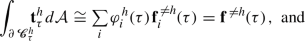 (D1a)
(D1a) -
(ii)
the surface integral of the tensor \(\textbf{r}(\cdot ,\tau )\!\otimes \!\textbf{t}^h_{\tau }\), where \(\textbf{r}(\varvec{z},\tau )\,\,{:=}\,\,\varvec{z}\!-\!\varvec{\chi }^{h}(\tau )\) for
 , is
\(\cong \)-equal to the total external moment (3.14) applied to (the particles in) the h-th cell:
, is
\(\cong \)-equal to the total external moment (3.14) applied to (the particles in) the h-th cell:
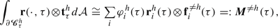 (D1b)
(D1b)with \(\textbf{r}_i^h(\tau )\,\,{:=}\,\,\varvec{q}_i(\tau )\!-\!\varvec{\chi }^{h}(\tau )\) (recall from (2.65) that \(\varvec{\chi }^{h}(\tau )\equiv \varvec{\chi }_{\tau }(\varvec{x}^h)\) is the center of
 ).
).

 , is
, is

 ).
).Statements (i) & (ii) are equivalent to the single assumption that

for all affine vector field \(\varvec{z}\mapsto \varvec{\alpha }(\varvec{z})=\varvec{v}+\varvec{L}(\varvec{z}\!-\!\varvec{\chi }^{h}(\tau ))\), with arbitrary \(\varvec{v}\) and \(\varvec{L}\). In fact, the left-hand and right-hand sides of (D2) read, respectively,Footnote 22

and
Recall from Sects. 2.2.1 and 2.3.2 that
 is well approximated by an open convex polyhedron (in the present context, a parallelepiped). Hence, each integral in (D1) splits into a sum of integrals over the polyhedron faces. Let
 be the interface separating two adjacent cells,
 and
and
 . Recall from Sects. 2.2.1 and 2.3.2 that
 is well approximated by a convex polygon having inner and outer diameters
\(\approx \!L_{\mathsf m}\) and edges whose length
\(\approx \!L_{\mathsf m}\). Hence, the contribution from the particles in an
\(L_{\mu }\,\)-neighborhood of the edges (or the vertices) of
is well approximated by a convex polygon having inner and outer diameters
\(\approx \!L_{\mathsf m}\) and edges whose length
\(\approx \!L_{\mathsf m}\). Hence, the contribution from the particles in an
\(L_{\mu }\,\)-neighborhood of the edges (or the vertices) of
 scales as
\(L_{\mathsf m}L_{\mu }\,^2\) (or as
\(L_{\mu }\,^3\)), while that from those in an
\(L_{\mu }\,\)-neighborhood of
scales as
\(L_{\mathsf m}L_{\mu }\,^2\) (or as
\(L_{\mu }\,^3\)), while that from those in an
\(L_{\mu }\,\)-neighborhood of
 scales as
\(L_{\mathsf m}^2L_{\mu }\,\). For this reason, the contributions from the particles not in
scales as
\(L_{\mathsf m}^2L_{\mu }\,\). For this reason, the contributions from the particles not in
 nor in
 but in an
\(L_{\mu }\,\)-neighborhood of the edges and vertices of
but in an
\(L_{\mu }\,\)-neighborhood of the edges and vertices of
 are negligible, and we may conclude that the external force applied to the particles close to
 from within the h-th cell is predominantly exerted by the particles close to
 from within the k-th cell. In the case of binary interactions, we may write

Swapping h with k and i with j in (D4) changes the sum on the right-hand side into its opposite, since \(\textbf{f}_{ji}\!=\!-\textbf{f}_{ij}\). Hence,

We may therefore associate the traction with the individual faces composing the boundary, provided that we endow them with an orientation. Let
 (
(
 ) be the face
 oriented with the unit normal vector
 (
(
 ) pointing outward of
 (
(
 ), with
 . Then, define

Given a point
 and a unit vector
\(\varvec{n}\), we could always design a tessellation such that, at a given time
\(\tau \), the face
and a unit vector
\(\varvec{n}\), we could always design a tessellation such that, at a given time
\(\tau \), the face
 common to two adjacent cells is centeredFootnote 23 at
\(\varvec{y}\) and normal to
\(\varvec{n}\). Let us label with k the cell toward which
\(\varvec{n}\) points and with h the other one. Under the assumption that, for every unit vector
\(\varvec{n}\), the field
\(\textbf{t}_{\tau }(\cdot ,\varvec{n})\) is approximately affine on the mesoscopic length scale
\(L_{\mathsf m}\) (recall definition in Sect. 2.2.2), equality (D5) combined with definitions (D6) yields
common to two adjacent cells is centeredFootnote 23 at
\(\varvec{y}\) and normal to
\(\varvec{n}\). Let us label with k the cell toward which
\(\varvec{n}\) points and with h the other one. Under the assumption that, for every unit vector
\(\varvec{n}\), the field
\(\textbf{t}_{\tau }(\cdot ,\varvec{n})\) is approximately affine on the mesoscopic length scale
\(L_{\mathsf m}\) (recall definition in Sect. 2.2.2), equality (D5) combined with definitions (D6) yields
for all
 and all unit vector
\(\varvec{n}\).
and all unit vector
\(\varvec{n}\).
On this basis, the Cauchy stress theorem—fundamental to continuum mechanics—can be proved [1]: for every
 , the traction
\(\textbf{t}_{\tau }(\varvec{y},\varvec{n})\) depends linearly on
\(\varvec{n}\). In other terms, there exists a tensor field, the Cauchy stress field
\(\textbf{T}_{\tau }\equiv \textbf{T}(\cdot ,\tau )\), smooth and approximately affine on the mesoscopic length scale
\(L_{\mathsf m}\), such that
, the traction
\(\textbf{t}_{\tau }(\varvec{y},\varvec{n})\) depends linearly on
\(\varvec{n}\). In other terms, there exists a tensor field, the Cauchy stress field
\(\textbf{T}_{\tau }\equiv \textbf{T}(\cdot ,\tau )\), smooth and approximately affine on the mesoscopic length scale
\(L_{\mathsf m}\), such that
Now, let
\(\textbf{n}^h_{\tau }\) denote the unit outer normal field on
 .Footnote 24 Then,

Substituting (D9) in the integral on the left-hand side of (D2) and using the divergence theoremFootnote 25 yields

since
\(\textbf{T}_{\tau }\) is approximately affine (and hence its divergence approximately constant) on the scale of
 ; moreover,
 . Comparing (D10) with (D3a) and (D1), we finally obtain expressions for the total external force
\(\textbf{f}^{\ne h}(\tau )\) and the total external moment
\(\varvec{M}^{\ne h}(\tau )\) acting on the h-th cell in terms of the Cauchy stress and its divergence at the cell center:
. Comparing (D10) with (D3a) and (D1), we finally obtain expressions for the total external force
\(\textbf{f}^{\ne h}(\tau )\) and the total external moment
\(\varvec{M}^{\ne h}(\tau )\) acting on the h-th cell in terms of the Cauchy stress and its divergence at the cell center:
where \(\mathcal {V}^h(\tau )\) is the current volume of the h-th cell. Substituting (D11a) and (D11b) in, respectively, (3.10a) and (3.10b), we get
The form of equations (D12b) suggests introducing the field \(\textbf{S}_{\tau }\!\!\equiv \!\textbf{S}(\cdot ,\tau )\), defined as the Piola transform of \(\textbf{T}_{\tau }\):
whose divergence enjoys the propertyFootnote 26
Substituting (D13) and (D14) in (D11) yields
i. e., equations (4.4).
Appendix E Running time averages
Definition and general properties Any integrable function f defined on a time interval \(\mathscr {I}\) whose duration \(\vert \mathscr {I}\vert \gg \!T\) can be split into the sum of its centered running \(\theta \)-average
with \(\theta \approx T\), and its \(\theta \)-fluctuating component
Of course, \(\overline{f'^{\theta }}^{\theta }\!\!=0\). Whenever \(\theta \) is clear from the context, we omit the superscript in \(\overline{f}^{\theta }\) and \(f'^{\theta }\). The bilinear product of two functions of time f, h satisfies the equality
Since both averaging and differentiating are linear operations, the time rate of the running average equals the running average of the time rate:
Running average of \(\,T\)-constant functions of time By definition (cf. Sect. 2.2.2), a function of time f is approximately constant on the T time scale (or T-constant) if
If f is T-constant, then it is \(\cong \)-equal to its running \(\theta \)-average for all \(\theta \approx T\) and, equivalently, its \(\theta \)-fluctuating component is \(\cong 0\):
Combining (E5) with (E3), we obtain that if at least one of two functions of time \(f,h\) is T-constant, then the running \(\theta \)-average of their product is \(\cong \)-equal to the product of their running \(\theta \)-averages, for all \(\theta \approx T\):
Any time interval \(\mathscr {I}\)such that \(\vert \mathscr {I}\vert \gg T\) can be subdivided into the disjoint union of a large number of subintervals \(\mathscr {I}_{_{1}},\dots ,\mathscr {I}_{_{\!S}}\) of duration \(\theta \approx T\), i. e.,
Let \(t_\iota \) be the middle point of \(\mathscr {I}_{\!\iota }\). Then, the integral of f over \(\mathscr {I}\) equals the sum over \(\iota \) of the integrals over \(\mathscr {I}_{\!\iota }\) of f, each of which equals \(\theta \overline{f}(t_\iota )\), due to (E1). If f is T-constant, then
on account of (E5). Hence,
Summing over \(\iota \), we obtain that the integral over \(\mathscr {I}\)of f is \(\cong \)-equal to the integral over \(\mathscr {I}\)of its running \(\theta \)-average \(\overline{f}\):
Combining (E10) with (E6), we obtain that the integral over \(\mathscr {I}\)of the bilinear product of two functions of time, of which one is T-constant, is \(\cong \)-equal to the integral of the product of their running \(\theta \)-averages:
Properties of essentially constant functions of time By definition (cf. Sect. 2.2.2), a function of time f is essentially constant if
If f is essentially constant, then it is \(\cong \)-equal to its running average \(\overline{f}\):
An essentially constant function of time f need not be continuous, let alone differentiable. However, there exists a time scale \(T_{f}\) such that, for all \(\theta \gtrapprox T_{f}\), the time derivative of its running \(\theta \)-average is zero to within a preset tolerance:
Appendix F Computing Lagrange multipliers
The i label being local to each representative cell, we rewrite (4.24) dropping the superscript h from \(\textbf{s}_i^h\) and its time derivatives. Premultiplying both sides of the equation by \({\textbf {F}}^{h}(t)^{-1}\) and reordering terms, we obtain
(recall that \(\textbf{f}_i(\tau )\) is computed as indicated in (4.2)). In each round of time integration of equations (F1), the initial state of the \(n^h\) representative particles populating the h-th cell can always be defined in such a way that
and that no particle leaves the cell at the initial time \(\tau _{_{0}}\). If (and only if) a particle sits initially on the cell boundary, at least one of its images also sits on the boundary. Moreover, if at time \(\tau _{_{0}}\) the thermal velocity of that particle points outward, then the thermal velocity of (at least) one of its images points inward. Therefore, it suffices to swap roles between particle and image to fix the initial conditions. Then, the time derivatives of constraints (2.78) at \(\tau _{_{0}}\) read
Substituting (F1) in (F3), taking into account (4.3), (4.5a), (F2), (3.14), (3.15), (2.88), (2.53), and (2.58) and using the fact that constraints (2.78) are satisfied at \(\tau _{_{0}}\), we get
with
Then, the solution to (F1) is propagated stepwise by a two-stage velocity Verlet algorithm [30, 31]:
where \(f_{n}\) stands for \(f(\tau _n)\) for each function of time f and each \(\tau _0,\tau _1,\dots \). The updated thermal velocity \(\dot{\textbf{s}}_{i(n+1)}\) is accepted as is, while the ‘scaled’ radius vector \(\textbf{s}_{i(n+1)}\) delivered by (F7) is accepted as final only if

i. e., if the i-th particle is still in
 at time
\(\tau _{n+1}\). Otherwise, it gets shifted by the unique linear combination of the edges of
at time
\(\tau _{n+1}\). Otherwise, it gets shifted by the unique linear combination of the edges of
 with coefficients taken in
\(\{0,\pm 1\}\), denoted
\(\textbf{u}_{i(n)}\), satisfying the condition
with coefficients taken in
\(\{0,\pm 1\}\), denoted
\(\textbf{u}_{i(n)}\), satisfying the condition

Since for \(\textbf{u}_{i(n)}\!=\varvec{0}\) (F10) coincides with (F9), in the following we take the (possibly) shifted update \(\textbf{s}_{i(n+1)}+\textbf{u}_{i(n)}\) as the scaled radius vector at time \(\tau _{n+1}\) of the i-th particle, be it the same particle as at time \(\tau _n\) or a new one.Footnote 27
Then, equations (F8) are solved expressing \(\dot{\textbf{s}}_{i(n+1)}\) ( \(i\!=\!1,\dots ,n^h\)) in terms of \(\varvec{\lambda }_{(n+1)}^{h}\) and \(\varvec{\Lambda }_{(n+1)}^{h}\), as follows:
where \({\textbf {C}}^{h}(t)={\textbf {F}}^{h}(t)^{\top }{\textbf {F}}^{h}(t)\), \(\textbf{A}^{\!h}(t)\!\,\,{:=}\,\,\big (\textbf{I}+\epsilon \big ({\textbf {F}}^{h}(t)^{-\top }\dot{{\textbf {F}}}^{h}(t)\big )^{\!-1}\!\), and
According to the SHAKE procedure [32,33,34], substituting (F11a) in the constraint equations (2.78) enforced at time \(\tau _{n+1}\), namely
we get
Under the assumption that
equations (F13) uncouple and deliver (the distinction between ‘equality’ and ‘equality to within a mesoscopically negligible error’ having been dismissed)
After substituting (F11b) in (F15), a simple but tedious calculation yields
on account of (4.3). The initial value (F4) entails
Then, after substituting (F7) and (F11b) in (F16), a calculation analogous to the one leading to (F17), but rather more tedious, yields
where
Combining (F19) with the initial value (F5), we see that \(\varvec{\Lambda }^{h}\) fluctuates around \({\textbf {F}}^{h}(t)^{\top }\ddot{{\textbf {F}}}^{h}(t)\). We remark that under PBCs, whenever a particle leaves the cell and one of its images enters it, the two simultaneous supplies of momentum compensate each other, while the corresponding supplies of moment of momentum do not, in general. This explains why \(\varvec{\Lambda }^{h}\) fluctuates, while \(\varvec{\lambda }^{h}\) does not (cf. (F18)).
Rights and permissions
Springer Nature or its licensor (e.g. a society or other partner) holds exclusive rights to this article under a publishing agreement with the author(s) or other rightsholder(s); author self-archiving of the accepted manuscript version of this article is solely governed by the terms of such publishing agreement and applicable law.
About this article

Cite this article
DiCarlo, A., Bonella, S., Ferrario, M. et al. Continuum mechanics from molecular dynamics via adiabatic time and length scale separation. Lett Math Phys 113, 24 (2023). https://doi.org/10.1007/s11005-022-01616-0
Received:
Revised:
Accepted:
Published:
DOI: https://doi.org/10.1007/s11005-022-01616-0