
Abstract
Multi-label classification extends the standard multi-class classification paradigm by dropping the assumption that classes have to be mutually exclusive, i.e., the same data item might belong to more than one class. Multi-label classification has many important applications in e.g. signal processing, medicine, biology and information security, but the analysis and understanding of the inference methods based on data with multiple labels are still underdeveloped. In this paper, we formulate a general generative process for multi-label data, i.e. we associate each label (or class) with a source. To generate multi-label data items, the emissions of all sources in the label set are combined. In the training phase, only the probability distributions of these (single label) sources need to be learned. Inference on multi-label data requires solving an inverse problem, models of the data generation process therefore require additional assumptions to guarantee well-posedness of the inference procedure. Similarly, in the prediction (test) phase, the distributions of all single-label sources in the label set are combined using the combination function to determine the probability of a label set. We formally describe several previously presented inference methods and introduce a novel, general-purpose approach, where the combination function is determined based on the data and/or on a priori knowledge of the data generation mechanism. This framework includes cross-training and new source training (also named label power set method) as special cases. We derive an asymptotic theory for estimators based on multi-label data and investigate the consistency and efficiency of estimators obtained by several state-of-the-art inference techniques. Several experiments confirm these findings and emphasize the importance of a sufficiently complex generative model for real-world applications.
1 Introduction
Multi-labelled data are encountered in classification of acoustic and visual scenes (Boutell et al. 2004), in text categorization (Joachims 1998; McCallum 1999), in medical diagnosis (Kawai and Takahashi 2009) and other application areas. For the classification of acoustic scenes, consider for example the well-known Cocktail-Party problem (Arons 1992), where several signals are mixed together and the objective is to detect the original signal. For a more detailed overview, we refer to Tsoumakas et al. (2010) and Zhang et al. (2013).
1.1 Prior art in multi-label learning and classification
In spite of its growing significance and attention, the theoretical analysis of multi-label classification is still in its infancy with limited literature. Some recent publications, however, show an interest to gain a fundamental insight into the problem of classifying multi-label data. Most attention is thereby attributed to correlations in the label sets. Using error-correcting output codes for multi-label classification (Dietterich and Bakiri 1995) has been proposed very early to “correct” invalid (i.e. improbable) label sets. The principle of maximum entropy is employed in Zhu et al. (2005) to capture correlations in the label set. The assumption of small label sets is exploited in the framework of compressed sensing by Hsu et al. (2009). Conditional random fields are used in Ghamrawi and McCallum (2005) to parameterize label co-occurrences. Instead of independent dichotomies, a series of classifiers is built in Read et al. (2009), where a classifier gets the output of all preceding classifiers in the chain as additional input. A probabilistic version thereof is presented in Dembczyński et al. (2010).
Two important gaps in the theory of multi-label classification have attracted the attention of the community in recent years: first, most research programs primarily focus on the label set, while an interpretation of how multi-label data arise is missing in the vast majority of the cases. Deconvolution problems (Streich 2010) define a special case of inference from multi-label data, as discussed in Chap. 2. In-depth analysis of the asymptotic behaviour of the estimators has been presented in Masry (1991, 1993). Secondly, a large number of quality measures has been presented, the understanding of how these are related with each other is underdeveloped. Dembczyński et al. (2012) analyses the interrelation between some of the most commonly used performance metrics. A theoretical analysis on the Bayes consistency of learning algorithm with respect to different loss functions is presented in Gao and Zhou (2013).
This contribution mainly addresses the issue how multi-label data are generated, i.e., we propose a generative model for multi-label data. A datum is composed of emissions by multiple sources. The emitting sources are indicated by the label set. These emissions are combined by a problem specific combination function like the linear superposition principle in optics or acoustics. The combination function specifies a core model assumption in the data generation process. Each source generates data items according to a source specific probability distribution. This point of view, as the reader should note, points into a direction that is orthogonal to the previously mentioned literature on label correlation: extra knowledge on the distribution of the label sets can coherently be represented by a prior over the label sets.
Furthermore, we assume that the sources are described by parametric distributions.Footnote 1 In this setting, the accuracy of the parameter estimators is a fundamental value to assess the quality of an inference scheme. This measure is of central interest in asymptotic theory, which investigates the distribution of a summary statistic in the asymptotic limit (Brazzale et al. 2007). Asymptotic analysis of parametric models has become an essential tool in statistics, as the exact distributions of the quantities of interest cannot be measured in most settings. In the first place, asymptotic analysis is used to check whether an estimation method is consistent, i.e. whether the obtained estimators converge to the correct parameter values if the number of data items available for inference goes to infinity. Furthermore, asymptotic theory provides approximate answers where exact ones are not available, namely in the case of data sets of finite size. Asymptotic analysis describes for example how efficiently an inference method uses the given data for parameter estimation (Liang and Jordan 2008).
Consistent inference schemes are essential for generative classifiers, and a more efficient inference scheme yields more precise classification results than a less efficient one, given the same training data. More specifically, the expected error of a classifier converges to the Bayes error for maximum a posteriori classification, if the estimated parameters converge to the true parameter values (Devroye et al. 1996). In this paper, we first review the state-of-the-art asymptotic theory for estimators based on single-label data. We then extend the asymptotic analysis to inference on multi-label data and prove statements about the identifiability of parameters and the asymptotic distribution of their estimators in this demanding setting.
1.2 Advantages of generative models
Generative models define only one approach to machine learning problems. For classification, discriminative models directly estimate the posterior distributions of class labels given data and, thereby, they avoid an explicit estimate of class specific likelihood distributions. A further reduction in complexity is obtained by discriminant functions, which map a data item directly to a set of classes or clusters (Hastie et al. 1993).
Generative models are the most demanding of all alternatives. If the only goal is to classify data in an easy setting, designing and inferring the complete generative model might be a wasteful use of resources and demand excessive amounts of data. However, namely in demanding scenarios, there exist well-founded reasons for generative models (Bishop 2007):
-
Generative description of data Even though this may be considered as stating the obvious, we emphasize that assumptions on the generative process underlying the observed data naturally enter into a generative model. Incorporating such prior knowledge into discriminative models proves typically significantly more difficult.
-
Interpretability The nature of multi-source data is best understood by studying how such data are generated. In most applications, the sources in the generative model come with a clear semantic meaning. Determining their parameters is thus not only an intermediate step to the final goal of classification, but an important piece of information on the structure of the data. Consider the cocktail party problem, where several speech and noise sources are superposed to the speech of the dialogue partner. Identifying the sources which generate the perceived signal is a demanding problem. The final goal, however, might go even further and consist of finding out what your dialogue partner said. A generative model for the sources present in the current acoustic situation enables us to determine the most likely emission of each source given the complete signal. This approach, referred to as model-based source separation (Hershey et al. 2010), critically depends on a reliable source model.
-
Reject option and outlier detection Given a generative model, we can also determine the probability of a particular data item. Samples with a low probability are called outliers. Their generation is not confidently represented by the generative model, and no reliable assignment of a data item to a set of sources is possible. Furthermore, outlier detection might be helpful in the overall system in which the machine learning application is integrated: outliers may be caused by defective measurement device or by fraud.
Since these advantages of generative models are prevalent in the considered applications, we restrict ourselves to generative methods when comparing our approaches with existing techniques.
1.3 A generative understanding of multi-label data
When defining a generative model, a distribution for each source has to be defined. To do so, one usually employs a parametric distribution, possibly based on prior knowledge or a study of the distribution of the data with a particular label. In the multi-label setting, the combination function is a further key component of the generative model. This function defines the semantics of the multi-label: while each single-labelled observation item is understood as a sample from a probability distribution identified by its label, multi-label observations are understood as a combination of the emissions of all sources in the label set. The combination function describes how the individual source emissions are combined to the observed data. Choosing an appropriate combination function is essential for successful inference and prediction. As we demonstrate in this paper, an inappropriate combination function might lead to inconsistent parameter estimators and worse label predictions, both compared to a simplistic approach where multi-label data items are ignored. Conversely, choosing the right combination function will allow us to extract more information from the training data, thus yielding more precise parameter estimators and superior classification accuracy.
The prominence of the combination function in the generative model naturally raises the question how this combination function can be determined. Specifying the combination function can be a challenging task when applying the deconvolutive method for multi-label classification. However, in our previous work, we achieved the insight that the combination function can typically be determined based on the data and prior knowledge, i.e. expertise in the field. For example in role mining, the disjunction of Boolean data is the natural choice (see Streich et al. 2009 for details), while the addition of (supposedly) Gaussian emissions is widely used in the classification of sounds (Streich and Buhmann 2008).
2 A generative model for multi-label data
We now present the generative process that we assume to have produced the observed data. Such generative models are widely found for single-label classification and clustering, but have not yet been formulated in a general form for multi-label data.
2.1 Label sets and source emissions
Let \(K\) denote the number of sources, and \(N\) the number of data items. We assume that the systematic regularities of the observed data are generated by a set \(\mathcal {K}= \{1,\ldots ,K\}\) of \(K\) sources. Furthermore, we assume that all sources have the same sample space \(\Omega \). Each source \(k \in \mathcal {K}\) emits samples \(\Xi _k \in \Omega \) according to a given parametric probability distributions \(P(\Xi _k|\theta _k)\), where \(\theta _k\) is the parameter tuple of source \(k\). Realizations of the random variables \(\Xi _k\) are denoted by \(\xi _k\). Note that both the parameters \(\theta _k\) and the emission \(\Xi _k\) can be vectors. In this case, \(\theta _{k,1}, \theta _{k,2},\ldots \) and \(\Xi _{k,1},\Xi _{k,2},\ldots \), denote different components of these vectors, respectively. Emissions of different sources are assumed to be independent of each other. The tuple of all source emissions is denoted by \(\varvec{\Xi } := (\Xi _1,\ldots ,\Xi _K)\), its probability distribution is given by \(P(\varvec{\Xi }|\varvec{\theta }) = \prod _{k=1}^K P(\Xi _k|\theta _k)\). The tuple of the parameters of all \(K\) sources is denoted by \(\varvec{\theta }:=(\theta _1,\ldots ,\theta _K)\).
Given an observation \(X=x\), the source set \(\mathcal {L}= \{ \lambda _1,\ldots ,\lambda _M\} \subseteq \mathcal {K}\) denotes the set of all sources involved in generating \(X\). The set of all possible label sets is denoted by \({\mathbb {L}}\). If \(\mathcal {L}= \{ \lambda \}\), i.e. \(|\mathcal {L}|=1\), \(X\) is called a single-label data item, and \(X\) is assumed to be a sample from source \(\lambda \). On the other hand, if \(|\mathcal {L}|>1\), \(X\) is called a multi-label data item and is understood as a combination of the emissions of all sources in the label set \(\mathcal {L}\). This combination is formalized by the combination function \(\mathrm c _{\kappa } : \Omega ^K \times {\mathbb {L}}\rightarrow \Omega \), where \(\kappa \) is a set of parameters the combination function might depend on. Note that the combination function only depends on emissions of sources in the label set and is independent of any other emissions.
The generative process \(\mathfrak {A}\) for a data item, as illustrated in Fig. 1, consists of the following three steps:
-
(1)
Draw a label set \(\mathcal {L}\) from the distribution \(P(\mathcal {L})\).
Fig. 1 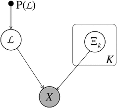
The generative model \(\mathfrak {A}\) for an observation \(X\) with source set \(\mathcal {L}\). An independent sample \(\Xi _k\) is drawn from each source \(k\) according to the distribution \(P(\Xi _k|\theta _k)\). The source set \(\mathcal {L}\) is sampled from the source set distribution \(P(\mathcal {L})\). These samples are then combined to observation by the combination function \(\mathrm c _{\kappa }(\varvec{\Xi }, \mathcal {L})\). Note that the observation \(X\) only depends on emissions from sources contained in the source set \(\mathcal {L}\)
-
(2)
For each \(k \in \mathcal {K}\), draw an independent sample \(\Xi _k \sim P(\Xi _k | \theta _k)\) from source \(k\). Set \(\varvec{\Xi } := (\Xi _1,\ldots ,\Xi _K)\).
-
(3)
Combine the source samples to the observation \(X = \mathrm c _{\kappa }(\varvec{\Xi }, \mathcal {L})\).

2.2 The combination function
The combination function models how emissions of one or several sources are combined to the structure component of the observation \(X\). Often, the combination function reflects a priori knowledge of the data generation process like the linear superposition law of electrodynamics and acoustics or disjunctions in role mining. For source sets of cardinality one, i.e. for single-label data, the combination function chooses the emission of the corresponding source: \(\mathrm c _{\kappa }(\varvec{\Xi }, \{\lambda \}) = \Xi _{\lambda }\).
For source sets with more than one source, the combination function can be either deterministic or stochastic. Examples for deterministic combination functions are the (weighted) sum and the Boolean OR operation. In this case, the value of \(X\) is completely determined by \(\varvec{\Xi }\) and \(\mathcal {L}\). In terms of probability distribution, a deterministic combination function corresponds to a point mass at \(X = \mathrm c _{\kappa }(\varvec{\Xi }, \mathcal {L})\):
Stochastic combination functions allow us to formulate e.g. the well-known mixture discriminant analysis as a multi-label problem (Streich 2010). However, stochastic combination functions render inference more complex, since a description of the stochastic behaviour of the function has to be learned in addition to the parameters of the source distributions. In the considered applications, deterministic combination functions suffice to model the assumed generative process. For this reason, we will not further discuss probabilistic combination functions in this paper.
2.3 Probability distribution for structured data
Given the assumed generative process \(\mathfrak {A}\), the probability of an observation \(X\) for source set \(\mathcal {L}\) and parameters \(\varvec{\theta }\) amounts to
We refer to \(P(X|\mathcal {L}, \varvec{\theta })\) as the proxy distribution of observations with source set \(\mathcal {L}\). Note that in the presented interpretation of multi-label data, the distributions \(P(X|\mathcal {L}, \varvec{\theta })\) for all source sets \(\mathcal {L}\) are derived from the single source distribution.
For a full generative model, we introduce \(\pi _{\mathcal {L}}\) as the probability of source set \(\mathcal {L}\). The overall probability of a data item \(D=(X,\mathcal {L})\) is thus
Several samples from the generative process are assumed to be independent and identically distributed (\(i.i.d.\)). The probability of \(N\) observations \(\varvec{X} =(X_1,\ldots , X_N)\) with source sets \(\varvec{\mathcal {L}}=(\mathcal {L}_1,\ldots ,\mathcal {L}_N)\) is thus \(P(\varvec{X}, \varvec{\mathcal {L}}|\varvec{\theta }) = \prod _{n=1}^N P(X_n,\mathcal {L}_n|\varvec{\theta })\). The assumption of \(i.i.d.\) data items allows us a substantial simplification of the model but is not a requirement for the assumed generative model.
To give an example of our generative model, we re-formulate the model used in McCallum (1999) in the terminology of this contribution. Omitting the mixture weights of individual classes within the label set (denoted by \(\varvec{\lambda }\) in the original contribution) and understanding a single document as a collection of \(W\) words, the probability of a single document is \(P(X) = \sum _{\mathcal {L}\in {\mathbb {L}}} P(\mathcal {L}) \prod _{w=1}^W \sum _{\lambda \in \mathcal {L}} P(X_w|\lambda )\). Comparing with the assumed data likelihood (Eq. 1), we find that the combination function is the juxtaposition, i.e. every word emitted by a source during the generative process will be found in the document.
A similar word-based mixture model for multi-label text classification is presented in Ueda and Saito (2006). Rosen-Zvi et al. (2004) introduce the author-topic model, a generative model for documents that combines the mixture model over words with Latent Dirichlet Allocation (Blei et al. 2003) to include authorship information: each author is associated with a multinomial distribution over topics and each topic is associated with a multinomial distribution over words. A document with multiple authors is modeled as a distribution over topics that is a mixture of the distributions associated with the authors. An additional dependency on the recipient is introduced in McCallum et al. (2005) in order to predict people’s roles from email communications. Yano et al. (2009) uses the topic model to predict the response to political blogs. We are not aware of any generative approaches to multi-label classification in other domains then text categorization.
2.4 Quality measures for multi-label classification
The quality measure mathematically formulates the evaluation criteria for the machine learning task at hand. A whole series of measures has been defined (Tsoumakas and Katakis 2007) to cover different requirements to multi-label classification. Commonly used are average precision, coverage, hamming loss, one-error and ranking loss (Schapire and Singer 2000; Zhang and Zhou 2006) as well as accuracy, precision, recall and F-Score (Godbole and Sarawagi 2004; Qi et al. 2007). We will focus on the balanced error rate (BER) (adapted from single-label classification) and precision, recall and F-score (inspired by information retrieval).
The BER is the ratio of incorrectly classified samples per label set, averaged (with equal weight) over all label sets:
While the BER considers the entire label set, precision and recall are calculated first per label. We first calculate the true positives \(tp_k = \sum _{n=1}^N ( 1_{\{k \in \hat{\mathcal {L}}_n\}} 1_{\{k \in \mathcal {L}_n\}} )\), false positives \(fp_k = \sum _{n=1}^N ( 1_{\{k \in \hat{\mathcal {L}}_n\}} 1_{\{k \notin \mathcal {L}_n\}} )\) and false negatives \(fn_k = \sum _{n=1}^N ( 1_{\{k \notin \hat{\mathcal {L}}_n\}} 1_{\{k \in \mathcal {L}_n\}} )\) for each class \(k\). The precision \(prec_k\) of class \(k\) is the fraction of data items correctly identified as belonging to \(k\), divided by the number of all data items identified as belonging to \(k\). The recall \(rec_k\) for a class \(k\) is the fraction of instances correctly recognized as belonging to this class, divided by the number of instances which belong to class \(k\):
Good performance with respect to either precision or recall alone can be obtained by either very conservatively assigning data items to classes (leading to typically small label sets and a high precision, but a low recall) or by attributing labels in a very generous way (yielding high recall, but low precision). The F-score \(F_k\), defined as the harmonic mean of precision and recall, finds a balance between the two measures:
Precision, recall and the F-score are determined individually for each base label \(k\). We report the average over all labels \(k\) (macro averaging). All these measures take values between 0 (worst) and 1 (best). The error rate and the BER are quality measures computed on an entire data set. Its values also range from 0 to 1, but here 0 is best.
Besides the quality criteria on the classification output, the accuracy of the parameter estimator compares the estimated source parameters with the true source parameters. This model-based criterion thus assesses the obtained solution of the essential inference problem in generative classification. However, a direct comparison between true and estimated parameters is typically only possible for experiments with synthetically generated data. The possibility to directly assess the inference quality and the extensive control over the experimental setting are actually the main reasons why, in this paper, we focus on experiments with synthetic data. We measure the accuracy of the parameter estimation by the mean square error (MSE), defined as the average squared distance between the true parameter \(\varvec{\theta }\) and its estimator \(\hat{\varvec{\theta }}\):
The MSE can be decomposed as follows:
The first term \({\mathbb {E}}_{\hat{\theta }_k}\![{|| \theta _{k,\cdot } - \hat{\theta }_{\pi (k), \cdot } ||}]\) is the expected deviation of the estimator \(\hat{\theta }_{\pi (k),\cdot }\) from the true value \(\theta _{k,\cdot }\), called the bias of the estimator. The second term \(\mathbb {V}_{\!\hat{\theta }_k}\![\hat{\theta }_k]\) indicates the variance of the estimator over different data sets. We will rely on this bias-variance decomposition when computing the asymptotic distribution of the mean-squared error of the estimators. In the experiments, we will report the root mean square error (RMS).
3 Preliminaries
Preliminaries to study the asymptotic behaviour of the estimators obtained by different inference methods are introduced in this section. This paper contains an elaborate notation, the probability distributions used are summarized in Table 1.
3.1 Exponential family distributions
In the following, we assume that the source distributions are members of the exponential family (Wainwright and Jordan 2008). This assumption implies that the distribution \(P_{\theta _k}(\Xi _k)\) of source \(k\) admits a density \(p_{\theta _k}(\xi _k)\) in the following form:
Here \(\theta _k\) are the natural parameters, \(\phi (\xi _k)\) are the sufficient statistics of the sample \(\xi _k\) of source \(k\), and \(A(\theta _k) := \log \left( \int \exp \left( \langle \theta _k, \phi (\xi _k)\rangle \right) {\,\mathrm d}\xi _k \right) \) is the log-partition function. The expression \(\langle \theta _k, \phi (\xi _k)\rangle := \sum _{s =1}^S \theta _{k,s} \cdot \left( \phi (\xi _k)\right) _s\) denotes the inner product between the natural parameters \(\theta _k\) and the sufficient statistics \(\phi (\xi _k)\). The number \(S\) is called the dimensionality of the exponential family. \(\theta _{k,s}\) is the \(s\mathrm{th }\) dimension of the parameter vector of source \(k\), and \(\left( \phi (\xi _k)\right) _s\) is the \(s\mathrm{th }\) dimension of the sufficient statistics. The (\(S\)-dimensional) parameter space of the distribution is denoted by \(\Uptheta \). The class of exponential family distributions contains many of the widely used probability distributions: the Bernoulli, Poisson and the \(\chi ^2\) distribution are one-dimensional exponential family distributions; the Gamma, Beta and normal distribution are examples of two-dimensional exponential family distributions.
The joint distribution of the independent sources is \(P_{\varvec{\theta }}(\varvec{\Xi }) = \prod _{k=1}^K P_{\varvec{\theta }_k}(\Xi _k) \), with the density function \(p_{\varvec{\theta }}(\varvec{\xi }) = \prod _{k=1}^K p_{\theta _k}(\xi _k)\). To shorten the notation, we define the vectorial sufficient statistic \(\varvec{\phi }(\varvec{\xi }) := (\phi (\xi _1),\ldots , \phi (\xi _K))^T\), the parameter vector \(\varvec{\theta }:=(\theta _1,\ldots ,\theta _K)^T\) and the cumulative log-partition function \(A(\varvec{\theta }) := \sum _{k=1}^K A(\theta _k)\). Using the parameter vector \(\varvec{\theta }\) and the emission vector \(\varvec{\xi }\), the density function \(p_{\varvec{\theta }}\) of the source emissions is \(p_{\varvec{\theta }}(\varvec{\xi }) = \prod _{k=1}^K p_{\theta _k}(\xi _k) = \exp \left( \langle \varvec{\theta }, \varvec{\phi }(\varvec{\xi })\rangle - A(\varvec{\theta })\right) \).
Exponential family distributions have the property that the derivatives of the log-partition function with respect to the parameter vector \(\varvec{\theta }\) are moments of the sufficient statistics \(\varvec{\phi }(\cdot )\). Namely the first and second derivative of \(A(\cdot )\) are the expected first and second moment of the statistics:
where \({\mathbb {E}}_{X\sim P\ }\!\left[ {X}\right] \) and \(\mathbb {V}_{\!X\sim P\ }\!\left[ X\right] \) denote the expectation value and the covariance matrix of a random variable \(X\) sampled from distribution \(P\). In all statements in this paper, we assume that all considered variances are finite.
3.2 Identifiability
The representation of exponential family distributions in Eq. 3 may not be unique, e.g. if the sufficient statistics \(\phi (\xi _k)\) are mutually dependent. In this case, the dimensionality \(S\) of the exponential family distribution can be reduced. Unless this is done, the parameters \(\theta _k\) are unidentifiable: there exist at least two different parameter values \(\theta _k^{(1)} \ne \theta _k^{(2)}\) which imply the same probability distribution \(p_{\theta _k^{(1)}}=p_{\theta _k^{(2)}}\). These two paramter values cannot be distinguished based on observations, they are therefore called unidentifiable (Lehmann and Casella 1998).
Definition 1
(Identifiability) Let \(\wp = \{ p_\theta : \theta \in \Theta \}\) be a parametric statistical model with parameter space \(\Theta \). \(\wp \) is called identifiable if the mapping \(\theta \rightarrow p_{\theta }\) is one-to-one: \(p_{\theta ^{(1)}} = p_{\theta ^{(2)}} \Longleftrightarrow \theta ^{(1)} = \theta ^{(2)}\) for all \(\theta ^{(1)}, \theta ^{(2)} \in \Theta \).
Identifiability of the model in the sense that the mapping \(\theta \rightarrow p_{\theta }\) can be inverted is equivalent to being able to learn the true parameters of the model if an infinite number of samples from the model can be observed (Lehmann and Casella 1998).
In all concrete learning problems, identifiability is always conditioned on the data. Obviously, if there are no observations from a particular source (class), the likelihood of the data is independent of the parameter values of the never-occurring source. The parameters of the particular source are thus unidentifiable.
3.3 \(M\)- and \(Z\)-estimators
A popular method to determine the estimators \(\hat{\varvec{\theta }} = (\hat{\theta }_1, \ldots , \hat{\theta }_K)\) for a generative model based on independent and identically-distributed (\(i.i.d.\)) data items \(\mathbf{D}= (D_1,\ldots ,D_N)\) is to maximize a criterion function \(\varvec{\theta } \mapsto M_N(\varvec{\theta }) = \frac{1}{N} \sum _{n=1}^N m_{\varvec{\theta }}(D_n)\), where \(m_{\varvec{\theta }} : \mathbf{D}\mapsto \mathbb R\) are known functions. An estimator \(\hat{\varvec{\theta }} = \arg \max _{\varvec{\theta }} M_N(\varvec{\theta })\) maximizing \(M_N(\varvec{\theta })\) is called an M-estimator, where \(M\) stands for maximization.
For continuously differentiable criterion functions, the maximizing value is often determined by setting the derivative with respect to \(\varvec{\theta }\) equal to zero. With \(\psi _{\varvec{\theta }}(D) := \nabla _{\varvec{\theta }} m_{\varvec{\theta }}(D)\), this yields an equation of the type \(\Psi _N(\varvec{\theta }) = \frac{1}{N} \sum _{n=1}^N \psi _{\varvec{\theta }}(D_n) \), and the parameter \(\varvec{\theta }\) is then determined such that \( \Psi _N(\varvec{\theta }) = 0\). This type of estimator is called Z-estimator, with \(Z\) standing for zero.
Maximum-likelihood estimators Maximum likelihood estimators are \(M\)-estimators with the criterion function \(m_{\varvec{\theta }}(D) := \ell (\varvec{\theta };D)\). The corresponding \(Z\)-estimator, which we will use in this paper, is obtained by computing the derivative of the log-likelihood with respect to the parameter vector \(\varvec{\theta }\), called the score:
Convergence Assume that there exists an asymptotic criterion function \(\varvec{\theta } \mapsto \Psi (\varvec{\theta })\) such that the sequence of criterion functions converges in probability to a fixed limit: \(\Psi _N(\varvec{\theta }) \mathop {\rightarrow }\limits ^{P} \Psi (\varvec{\theta })\) for every \(\varvec{\theta }\). Convergence can only be obtained if there is a unique zero \(\varvec{\theta }_0\) of \(\Psi (\cdot )\), and if only parameters \(\varvec{\theta }\) close to \(\varvec{\theta }_0\) yield a value of \(\Psi (\varvec{\theta })\) close to zero. Thus, \(\varvec{\theta }_0\) has to be a well-separated zero of \(\Psi (\cdot )\) (van der Vaart 1998):
Theorem 1
Let \(\Psi _N\) be random vector-valued functions and let \(\Psi \) be a fixed vector-valued function of \(\varvec{\theta }\) such that for every \(\epsilon >0\)
Then any sequence of estimators \(\hat{\varvec{\theta }}_N\) such that \(\Psi _N(\hat{\varvec{\theta }}_N) = o_P \left( 1 \right) \) converges in probability to \(\varvec{\theta }_0\).
The notation \(o_P \left( 1 \right) \) denotes a sequence of random vectors that converges to 0 in probability, and \(d(\varvec{\theta },\varvec{\theta }_0)\) indicates the Euclidian distance between the estimator \(\varvec{\theta }\) and the true value \(\varvec{\theta }_0\). The second condition implies that \(\varvec{\theta }_0\) is the only zero of \(\Psi (\cdot )\) outside a neighborhood of size \(\epsilon \) around \(\varvec{\theta }_0\). As \(\Psi (\cdot )\) is defined as the derivative of the likelihood function (Eq. 5), this criterion is equivalent to a concave likelihood function over the whole parameter space \(\Uptheta \). If the likelihood function is not concave, there are several (local) optima, and convergence to the global maximizer \(\varvec{\theta }_0\) cannot be guaranteed.
Asymptotic normality Given consistency, the question about how the estimators \(\hat{\varvec{\theta }}_N\) are distributed around the asymptotic limit \(\varvec{\theta }_0\) arises. Assuming the criterion function \(\varvec{\theta } \mapsto \psi _{\varvec{\theta }}(D)\) to be twice continuously differentiable, \(\Psi _N(\hat{\varvec{\theta }}_N)\) can be expanded through a Taylor series around \(\varvec{\theta }_0\). Then, using the central limit theorem, \(\hat{\varvec{\theta }}_N\) is found to be normally distributed around \(\varvec{\theta }_0\) (van der Vaart 1998). Defining \(\varvec{v}^{\otimes } := \varvec{v} \varvec{v}^T\), we get the following theorem (all expectation values w.r.t. the true distribution of the data items \(D\)):
Theorem 2
Assume that \({\mathbb {E}}_{D}\!\left[ {\psi _{\varvec{\theta }_0}(D)^{\otimes }}\right] < \infty \) and that the map \(\varvec{\theta } \mapsto {\mathbb {E}}_{D}\!\left[ {\psi _{\varvec{\theta }}(D)}\right] \) is differentiable at a zero \(\varvec{\theta }_0\) with non-singular derivative matrix. Then, the sequence \(\sqrt{N} \cdot (\hat{\varvec{\theta }}_N - \varvec{\theta }_0)\) is asymptotically normal: \( \sqrt{N} \cdot (\hat{\varvec{\theta }}_N - \varvec{\theta }_0) \rightarrow \mathcal {N}(0, \Sigma ) \) with asymptotic variance
3.4 Maximum-likelihood estimation on single-label data
To estimate parameters on single-label data, a data set \(\mathbf{D}=\{(X_n, \lambda _n) \}\), \(n=1,\ldots , N\), with \(\lambda _n \in \{1,\ldots ,K\}\) for all \(n\), is separated according to the class label, so that one gets \(K\) sets \(\mathbf{X}_1,\ldots ,\mathbf{X}_K\), where \(\mathbf{X}_k := \{ X_n | (X_n, \lambda _n) \in \mathbf{D}, \lambda _n = k \}\) contains all observations with label \(k\). All samples in \(\mathbf{X}_k\) are assumed to be \(i.i.d.\) random variables distributed according to \(P(X|\theta _k)\). It is assumed that the samples in \(\mathbf{X}_k\) do not provide any information about \(\theta _{k'}\) if \(k \ne k'\), i.e. parameters for the different classes are functionally independent of each other (Duda et al. 2000). Therefore, we obtain \(K\) independent parameter estimation problems, each with criterion function \(\Psi _{N_k}(\theta _k) = \frac{1}{N_k} \sum _{X \in \mathbf{X}_k} \psi _{\theta _k}( (X,k) ) \), where \(N_k := |\mathbf{X}_k|\). The parameter estimator \(\hat{\theta }_k\) is then determined such that \(\Psi _{N_k}(\theta _k)=0\). More specifically for maximum-likelihood estimation of parameters of exponential family distributions (Eq. 3), the criterion function \(\psi _{\theta _k}(D) = \nabla _{\varvec{\theta }} \ell (\varvec{\theta };D)\) (Eq. 5) for a data item \(D=(X,\{k\})\) becomes \(\psi _{\theta _k}(D) = \phi (X) - {\mathbb {E}}_{\Xi _k \sim P_{\theta _k}}\!\left[ {\phi (\Xi _k)}\right] \). Choosing \(\hat{\theta }_k\) such that the criterion function \(\Psi _{N_k}(\theta _k)\) is zero means changing the model parameter such that the average value of the sufficient statistics of the observations coincides with the expected sufficient statistics:
Hence, maximum-likelihood estimators in exponential families are moment estimators (Wainwright and Jordan 2008). The theorems of consistency and asymptotic normality are directly applicable.
With the same formalism, it becomes clear why the inference problems for different classes are independent: assume an observation \(X\) with label \(k\) is given. Under the assumption of the generative model, the label \(k\) states that \(X\) is a sample from source \(p_{\theta _k}\). Trying to derive information about the parameter \(\theta _{k'}\) of a second source \(k' \ne k\) from \(X\), we would derive \(p_{\theta _k}\) with respect to \(\theta _{k'}\) to get the score function. Since \(p_{\theta _k}\) is independent of \(\theta _{k'}\), this derivative is zero, and the data item \((X,k)\) does not contribute to the criterion function \(\Psi _{N_{k'}}(\theta _{k'})\) (Eq. 7) for \(\theta _{k'}\).
Fisher information For inference in a parametric model with a consistent estimator \(\hat{\theta }_k \rightarrow \theta _k\), the Fisher information \(\mathcal {I}\) (Fisher 1925) is defined as the second moment of the score function. Since the parameter estimator \(\hat{\theta }\) is chosen such that the average of the score function is zero, the second moment of the score function corresponds to its variance:
where the expectation is taken with respect to the true distribution \(P_{\theta ^G_k}\). The Fisher information thus indicates to what extend the score function depends on the parameter. The larger this dependency is, the more the observed data depends on the parameter value, and the more accurately this parameter value can be determined for a given set of training data. According to the Cramér–Rao bound (Rao 1945; Cramér 1946, 1999), the reciprocal of the Fisher information is a lower bound on the variance of any unbiased estimator of a deterministic parameter. An estimator \(\hat{\theta }_k \) is called efficient if \(\mathbb {V}_{X \sim P_{\theta ^G_k}} [\hat{\theta }_k] = ( \mathcal {I}_{\mathbf{X}_k}(\theta _k) )^{-1}\).
4 Asymptotic distribution of multi-label estimators
We now extend the asymptotic analysis to estimators based on multi-label data. We restrict ourselves to maximum likelihood estimators for the parameters of exponential family distributions. As we are mainly interested in comparing different ways to learn from data, we also assume the parametric form of the distribution to be known.
4.1 From observations to source emissions
In single-label inference problems, each observation provides a sample of a source indicated by the label, as discussed in Sect. 3.4. In the case of inference based on multi-label data, the situation is more involved, since the source emissions cannot be observed directly. The relation between the source emissions and the observations are formalized by the combination function (see Sect. 2) describing the observation \(X\) based on an emission vector \(\varvec{\Xi }\) and the label set \(\mathcal {L}\).
To perform inference, we have to determine which emission vector \(\varvec{\Xi }\) has produced the observed \(X\). To solve this inverse problem, an inference method relies on additional constraints besides assuming the parametric form of the distribution, namely on the combination function. These design assumptions — made implicitly or explicitly — enable the inference scheme to derive information about the distribution of the source emissions given an observation.
In this analysis, we focus on differences in the assumed combination function. \(P^{\mathcal {M}}(X|\varvec{\Xi }, \mathcal {L})\) denotes the probabilistic representations of the combination function: it specifies the probability distribution of an observation \(X\) given the emission vector \(\varvec{\Xi }\) and the label set \(\mathcal {L}\), as assumed by method \(\mathcal {M}\). We formally describe several techniques along with the analysis of their estimators in Sect. 5. It is worth mentioning that for single-label data, all estimation techniques considered in this work are equal and yield consistent and efficient parameter estimators, as they agree on the combination function for single-label data: the identity function is the only reasonable choice in this case.
The probability distribution of \(X\) given the label set \(\mathcal {L}\), the parameters \(\varvec{\theta }\) and the combination function assumed by method \(\mathcal {M}\) is computed by marginalizing \(\varvec{\Xi }\) out of the joint distribution of \(\varvec{\Xi }\) and \(X\):
For the probability of a data item \(D=(X,\mathcal {L})\) given the parameters \(\varvec{\theta }\) and under the assumptions made by model \(\mathcal {M}\), we have
Estimating the probability of the label set \(\mathcal {L}\), \(\pi _{\mathcal {L}}\), is a standard problem of estimating the parameters of a categorical distribution. According to the law of large numbers, the empirical frequency of occurrence converges to the true probability for each label set. Therefore, we do not further investigate this estimation problem and assume that the true value of \(\pi _{\mathcal {L}}\) can be determined for all \(\mathcal {L}\in {\mathbb {L}}\).
The probability of a particular emission vector \(\varvec{\Xi }\) given a data item \(D\) and the parameters \(\varvec{\theta }\) is computed using Bayes’ theorem:
The dependency of \(\varvec{\theta }\) on the parameter vector \(\varvec{\theta }\) indicates that the estimation of the contributions of a source may depend on the parameters of a different source. When solving clustering problems, we also find cross-dependencies between parameters of different classes. However, these dependencies are due to the fact that the class assignments are not known but are probabilistically estimated. If the true class labels were known, the dependencies would disappear. In the context of multi-label classification, however, the mutual dependencies persist even when the true labels (called label set in our context) are known.
The distribution \(P^{\mathcal {M}}(\varvec{\Xi }|D,\varvec{\theta })\) describes the essential difference between inference methods for multi-label data. For an inference method \(\mathcal {M}\) which assumes that an observation \(X\) is a sample from each source contained in the label set \(\mathcal {L}\), \(P^{\mathcal {M}}(\Xi _k|D,\varvec{\theta })\) is a point mass (Dirac mass) at \(X\). In the above example of the sum of Gaussian emissions, \(P^{\mathcal {M}}(\varvec{\Xi }|D,\varvec{\theta })\) has a continuous density function.
4.2 Conditions for identifiability
As in the standard scenario of learning from single-label data, parameter inference is only possible if the parameters \(\varvec{\theta }\) are identifiable. Conversely, parameters are unidentifiable if \(\varvec{\theta }^{(1)} \ne \varvec{\theta }^{(2)}\), but \(P_{\varvec{\theta }^{(1)}}= P_{\varvec{\theta }^{(2)}}\). For our setting as specified in Eq. 9, this is the case if
but \(\varvec{\theta }^{(1)} \ne \varvec{\theta }^{(2)}\). The following situations imply such a scenario:
-
A particular source \(k\) never occurs in the label set, formally \(\left| \{ \mathcal {L}\in {\mathbb {L}}| k \in \mathcal {L}\} \right| = 0\) or \(\pi _{\mathcal {L}}= 0 \quad \forall \mathcal {L}\in {\mathbb {L}}: \mathcal {L}\ni k\). This excess parameterization is the trivial case — one cannot infer the parameters of a source without observing emissions from that source. In such a case, the probability of the observed data (Eq. 9) is invariant of the parameters \(\theta _k\) of source \(k\).
-
The combination function ignores all (!) emissions of a particular source \(k\). Thus, under the assumptions of the inference method \(\mathcal {M}\), the emission \(\Xi _k\) of source \(k\) never has an influence on the observation. Hence, the combination function does not depend on \(\Xi _k\). If this independence holds for all \(\mathcal {L}\), information on the source parameters \(\theta _k\) cannot be obtained from the data.
-
The data available for inference does not support distinguishing different parameters of a pair of sources. Assume e.g. that source \(2\) only occurs together with source \(1\), i.e. for all \(n\) with \(2 \in \mathcal {L}_n\), we also have \(1 \in \mathcal {L}_n\). Unless the combination function is such that information can be derived about the emissions of the two sources \(1\) and \(2\) for at least some of the data items, there is a set of parameters \(\theta _1\) and \(\theta _2\) for the two sources that yields the same likelihood.
If the distribution of a particular source is unidentifiable, the chosen representation is problematic for the data at hand and might e.g. contain redundancies, such as a source (class) which is never observed. More specifically, in the first two cases, there does not exist any empirical evidence for the existence of a source which is either never observed or has no influence on the data. In the last case, one might doubt if the two classes \(1\) and \(2\) are really separate entities, or whether it might be more reasonable to merge them to a single class. Conversely, non-compliance to the three above conditions is a necessary (but not sufficient!) condition for parameter identifiability in the model.
4.3 Maximum likelihood estimation on multi-label data
Based on the probability of a data item \(D\) given the parameter vector \(\varvec{\theta }\) under the assumptions of the inference method \(\mathcal {M}\) (Eq. 9) and using a uniform prior over the parameters, the log-likelihood of a parameter \(\varvec{\theta }\) given a data item \(D=(X,\mathcal {L})\) is given by \( \ell ^{\mathcal {M}}(\varvec{\theta };D) = \log ( P^{\mathcal {M}}(X,\mathcal {L}|\varvec{\theta }) ) \). Using the particular properties of exponential family distributions (Eq. 4), the score function is
Comparing with the score function obtained in the single-label case (Eq. 7), the difference in the first term becomes apparent. While the first term is the sufficient statistic of the observation in the previous case, we now find the expected value of the sufficient statistic of the emissions, conditioned on \(D=(X,\mathcal {L})\). This formulation contains the single-label setting as a special case: given the single-label observation \(X\) with label \(k\), we are sure that the \(k\)th source has emitted \(X\), i.e. \(\Xi _k=X\). In the more general case of multi-label data, several emission vectors \(\varvec{\Xi }\) might have produced the observed \(X\). The distribution of these emission vectors (\(D\) and \(\varvec{\theta }\)) is given by Eq. 10. The expectation of the sufficient statistics of the emissions with respect to this distribution now plays the role of the sufficient statistic of the observation in the single-label case.
As in the single-label case, we assume that several emissions are independent given their sources (conditional independence). The likelihood and the criterion function for a data set \(\mathbf{D}=(D_1,\ldots ,D_N)\) thus factorize:
In the following, we study \(Z\)-estimators \(\hat{\varvec{\theta }}_N^{\mathcal {M}}\) obtained by setting \(\Psi _N^{\mathcal {M}}(\hat{\varvec{\theta }}{}^{\mathcal {M}}_N) = 0\). We analyse the asymptotic behaviour of the criterion function \(\Psi _N^{\mathcal {M}}\) and derive conditions for consistent estimators as well as their convergence rates.
4.4 Asymptotic behaviour of the estimation equation
We analyse the criterion function in Eq. 13. The \(N\) observations used to estimate \(\Psi _N^{\mathcal {M}}(\varvec{\theta }_0^{\mathcal {M}})\) originate from a mixture distribution specified by the label sets. Using the \(i.i.d.\) assumption and defining \(\mathbf{D}_{\mathcal {L}} := \{(X',\mathcal {L}') \in \mathbf{D}| \mathcal {L}' = \mathcal {L}\}\), we derive
Denote by \(P_{\mathcal {L}, \mathbf{D}}\) the empirical distribution of observations with label set \(\mathcal {L}\). Then,
is an average of independent, identically distributed random variables. By the law of large numbers, this empirical average converges to the true average as the number of data items, \(N_{\mathcal {L}}\), goes to infinity:
Furthermore, define \(\hat{\pi }_{\mathcal {L}} := {N_{\mathcal {L}}}/N\). Again by the law of large numbers, we get \(\hat{\pi }_{\mathcal {L}} \rightsquigarrow \pi _{\mathcal {L}}\). Inserting (15) into (14), we derive
Inserting the value of the score function (Eq. 12) into Eq. 16 yields
This expression shows that the maximum likelihood estimator is a moment estimator also for inference based in multi-label data. However, the source emissions cannot be observed directly, and the expected value of its sufficient statistic substitutes for this missing information. The average is taken with respect to the distribution of the source emissions assumed by the inference method \(\mathcal {M}\).
4.5 Conditions for consistent estimators
Estimators are characterized by properties like consistency and efficiency. The following theorem specifies conditions under which the estimator \(\hat{\varvec{\theta }} \ \!_N^{\mathcal {M}}\) is consistent.
Theorem 3
(Consistency of estimators.) Assume the inference method \(\mathcal {M}\)uses the true conditional distribution of the source emissions \(\varvec{\Xi }\) given data items, i.e. for all data items \(D=(X,\mathcal {L})\), \(P^{\mathcal {M}}(\varvec{\Xi } | (X,\mathcal {L}),\varvec{\theta } ) = P^G(\varvec{\Xi }|(X,\mathcal {L}),\varvec{\theta })\), and that \(P^{\mathcal {M}}(\varvec{X} | \mathcal {L},\varvec{\theta })\) is concave. Then the estimator \(\hat{\varvec{\theta }}\) determined as a zero of \(\Psi _N^{\mathcal {M}}(\varvec{\theta })\) (Eq. 17) is consistent.
Proof
The true parameter of the generative process, denoted by \(\varvec{\theta }^G\), is a zero of \(\Psi ^G(\varvec{\theta })\), the criterion function derived from the true generative model. According to Theorem 1, \(\sup _{\varvec{\theta } \in \varvec{\Theta }} || \Psi ^{\mathcal {M}}_N(\varvec{\theta }) - \Psi ^G(\varvec{\theta })|| \mathop {\rightarrow }\limits ^{P} 0\) is a necessary condition for consistency of \(\hat{\varvec{\theta }}{}_N^{\mathcal {M}}\). Inserting the criterion function \(\Psi ^{\mathcal {M}}_N(\varvec{\theta })\) (Eq. 17) yields the condition
Splitting the generative process for the data items \(D \sim P_{\varvec{\theta }^G}\) into a separate generation of the label set \(\mathcal {L}\) and an observation \(X\), \(\mathcal {L}\sim P_{\pi ^G}\), \(X \sim P_{\mathcal {L}, \varvec{\theta }^G}\), Eq. 18 is fulfilled if
Using the assumption that \(P_{(X,\mathcal {L}),\varvec{\theta }}^{\mathcal {M}} = P_{(X,\mathcal {L}),\varvec{\theta }}^G\) for all data items \(D=(X,\mathcal {L})\), this condition is trivially fulfilled. \(\square \)
Differences between \(P_{D^{\delta },\varvec{\theta }}^{\mathcal {M}}\) and \(P_{D^{\delta },\varvec{\theta }}^G\) for some data items \(D^{\delta } = (X^{\delta }, \mathcal {L}^{\delta })\), on the other hand, have no effect on the consistency of the result if either the probability of \(D^{\delta }\) is zero, or if the expected value of the sufficient statistics is identical for the two different parameter vectors. The first situation implies that either the label set \(\mathcal {L}^{\delta }\) never occurs in any data item, or the observation \(X^{\delta }\) never occurs with label set \(\mathcal {L}^{\delta }\). The second situation implies that the parameters are unidentifiable. Hence, we formulate the stronger conjecture that if an inference procedure yields inconsistent estimators on data with a particular label set, its overall parameter estimators are inconsistent. This implies, in particular, that inconsistencies on two (or more) label sets cannot compensate each other to yield an estimator which is consistent on the entire data set.
As we show in Sect. 5, ignoring all multi-label data yields consistent estimators. However, discarding a possibly large part of the data is not efficient, which motivates the quest for more advanced inference techniques to retrieve information of the source parameters from multi-label data.
4.6 Efficiency of parameter estimation
Given that an estimator \(\hat{\varvec{\theta }}\) is consistent, the next question of interest concerns the rate at which the deviation from the true parameter value converges to zero. This rate is given by the asymptotic variance of the estimator (Eq. 6). We will compute the asymptotic variance specifically for maximum likelihood estimators in order to compare different inference techniques which yield consistent estimators in terms of how efficiently they use the provided data set for inference.
Fisher information The Fisher information is introduced to measure the information content of a data item for the parameters of the source that is assumed to have generated the data. In multi-label classification, the definition of the Fisher information (Eq. 8) has to be extended, as the source emissions are only indirectly observed:
Definition 2
Fisher information of multi-label data The Fisher information \(\mathcal {I}_{\mathcal {L}}\) measures the amount of information a data item \(D=(X,\mathcal {L})\) with label set \(\mathcal {L}\) contain about the parameter vector \(\varvec{\theta }\):
The term \(\mathbb {V}_{\!\varvec{\Xi }\sim P_{D,\varvec{\theta }}^{\mathcal {M}}}\!\left[ \varvec{\phi }(\varvec{\Xi })\right] \) measures the uncertainty about the emission vector \(\varvec{\Xi }\), given a data item \(D\). This term vanishes if and only if the data item \(D\) completely determines the source emission(s) of all involved sources. In the other extreme case where the data item \(D\) does not reveal any information about the source emissions, this is equal to \(\mathbb {V}_{\!\varvec{\Xi } \sim P_{\varvec{\theta }}}\!\left[ \varvec{\phi }(\varvec{\Xi })\right] \), and the Fisher information vanishes.
Asymptotic variance We now determine the asymptotic variance of an estimator.
Theorem 4
(Asymptotic variance.) Denote by \(P_{D,\varvec{\theta }}^{\mathcal {M}}(\varvec{\Xi })\) the distribution of the emission vector \(\varvec{\Xi }\) given the data item \(D\) and the parameters \(\varvec{\theta }\), under the assumptions made by the inference method \(\mathcal {M}\). Furthermore, let \(\mathcal {I}_{\mathcal {L}}\) denote the Fisher information of data with label set \(\mathcal {L}\). Then, the asymptotic variance of the maximum likelihood estimator \(\hat{\varvec{\theta }}\) is given by
where all expectations and variances are computed with respect to the true distribution.
Proof
We derive the asymptotic variance based on Theorem 2 on asymptotic normality of \(Z\)-estimators. The first and last factor in Eq. 6 are the derivative of the criterion function \(\psi _{\varvec{\theta }}^{\mathcal {M}}(D)\) (Eq. 11):
where \(\varvec{v}^{\otimes }\) denotes the outer product of vector \(\varvec{v}\). The particular properties of the exponential family distributions imply
with \( \nabla P^{\mathcal {M}}_{\varvec{\theta }}(D) / P^{\mathcal {M}}_{\varvec{\theta }}(D) = \psi _{\varvec{\theta }}^{\mathcal {M}}(D)\) and using Eq. 12, we get
The expected Fisher information matrix over all label sets results from computing the expectation over the data items \(D\):
For the middle term of Eq. 6, we have
The condition for \(\hat{\varvec{\theta }}\) given in Eq. 17 implies
Using Eq. 6, we derive the expression for the asymptotic variance of the estimator \(\varvec{\theta }\) stated in the theorem. \(\square \)
According to this result, the asymptotic variance of the estimator is determined by two factors. We analyse them in the following two subsections and afterwards derive some well-known results for special cases.
(A) Bias-variance decomposition
We define the expectation-deviance for label set \(\mathcal {L}\) as the difference between the expected value of the sufficient statistics under the distribution assumed by method \(\mathcal {M}\), given observations with label set \(\mathcal {L}\), and the expected value of the sufficient statistic given all data items:
The middle factor (Eq. 22) of the estimator variance is the variance in the expectation values of the sufficient statistics of \(\varvec{\Xi }\). Using \({\mathbb {E}}_{X}\!\left[ {X^2}\right] ={\mathbb {E}}_{X}\!\left[ {X}\right] ^2+\mathbb {V}_{\!X}\!\left[ X\right] \) and splitting \(D=(X,\mathcal {L})\) into the observation \(X\) and the label set \(\mathcal {L}\), it can be decomposed as
Two independent effects thus cause a high variance of the estimator:
-
(1)
The expected value of the sufficient statistics of the source emissions based on observations with a particular label \(\mathcal {L}\) deviates from the true parameter value. Note that this effect can be present even if the estimator is consistent: these deviations of sufficient statistics conditioned on a particular label set might cancel out each other when averaging over all label sets and thus yield a consistent estimator. However, an estimator obtained by such a procedure has a higher variance than an estimator which is obtained by a procedure which yields consistent estimators also conditioned on every label set.
-
(2)
The expected value of the sufficient statistics of the source emissions given the observation \(X\) varies with \(X\). This contribution is typically large for one-against-all methods (Rifkin and Klautau 2004).
Note that for inference methods which fulfil the conditions of Theorem 3, we have \(\Delta {\mathbb {E}}_{\mathcal {L}}^{\mathcal {M}}=0\). Methods which yield consistent estimators on any label set are thus not only provably consistent, but also yield parameters with less variation.
(B) Special cases
The above result reduces to well-known formula for some special cases of single label assignments.
Variance of estimators on single-label data If estimation is based on single-label data, i.e. \(D=(X,\mathcal {L})\) and \(\mathcal {L}=\{\lambda \}\), the source emissions are fully determined by the available data, as the observations are considered to be direct emissions of the respective source.
The estimation procedure is thus independent for every source \(k\). Furthermore, we have \({\mathbb {E}}_{\Xi _k \sim P_{D,\theta _k}^{\mathcal {M}}}\![{\phi (\Xi _k)}] = X\) and \(\mathbb {V}_{\!\Xi _k\sim P_{D,\theta _k}^{\mathcal {M}}}\![\phi (\Xi _k)] = 0\). Hence, \(\Sigma \) is a diagonal matrix, with diagonal elements
Variance of consistent estimators Consistent estimators are characterized by the expression \({\mathbb {E}}_{D\sim P_{\varvec{\theta }^G}}\!\left[ { {\mathbb {E}}_{\varvec{\Xi }\sim P_{D,\varvec{\theta }}^{\mathcal {M}}}\!\left[ {\varvec{\phi }(\varvec{\Xi })}\right] }\right] = {\mathbb {E}}_{\varvec{\Xi }\sim P_{\varvec{\theta }}}\!\left[ {\varvec{\phi }(\varvec{\Xi })}\right] \) and thus
Variance of consistent estimators on single-label data Combining the two aforementioned conditions, we derive
which corresponds to the well-known result for single-label data (Eq. 8).
5 Asymptotic analysis of multi-label inference methods
In this section, we formally describe several techniques for inference based on multi-label data and apply the results obtained in Sect. 4 to study the asymptotic behaviour of estimators obtained with these methods.
5.1 Ignore training (\(\mathcal {M}_{ignore}\))
The ignore training is probably the simplest, but also the most limited way of treating multi-label data: data items which belong to more than one class are simply ignored (Boutell et al. 2004), i.e. the estimation of source parameters is uniquely based on single-label data. The overall probability of an emission vector \(\varvec{\Xi }\) given the data item \(D\) thus factorizes:
Each of the factors \(P_{D,\varvec{\theta },k}^{ignore}(\Xi _k)\), representing the probability distribution of source \(k\), only depends on the parameter \(\theta _k\), i.e. we have \(P_{D,\varvec{\theta },k}^{ignore}(\Xi _k) = P_{D,\theta _k}^{ignore}(\Xi _k)\) for all \(k=1,\ldots ,K\). A data item \(D=(X,\mathcal {L})\) does exclusively provide information about source \(k\) if \(\mathcal {L}= \{k\}\). In the case \(\mathcal {L}\ne \{k\}\), the probability distribution of emissions \(\Xi _k\), \(P_{D,\hat{\theta }_k}^{ignore}(\Xi _k)\), is invariant to data item \(D\).
Observing a multi-label data items does not change the assumed probability distribution of any of the classes, as these data items are discarded by \(\mathcal {M}_{ignore}\). From Eqs. 26 and 27, we obtain the following criterion function given a data item \(D\):
The estimator \(\hat{\varvec{\theta }}{}^{ignore}\) is consistent and normally distributed:
Lemma 1
The estimator \(\hat{\varvec{\theta }}{}^{ignore}_N\) determined as a zero of \(\Psi _N^{ignore}(\varvec{\theta })\) as defined in Eqs. 13 and 28 is distributed according to \(\sqrt{N} \cdot (\hat{\varvec{\theta }}{}_N^{ignore} - \varvec{\theta }^G) \rightarrow \mathcal {N}(0, \Sigma ^{ignore})\). The covariance matrix \(\Sigma ^{ignore}\) is given by \(\Sigma ^{ignore} = \mathrm diag (\Sigma ^{ignore}_{11}, \ldots , \Sigma ^{ignore}_{KK} )\), with \(\Sigma ^{ignore}_{kk} = \mathbb {V}_{\!X \sim P_{\theta _k}}\![\psi _{\theta _k}^{ignore}((X, \{k\}))]^{-1}\).
This statement follows directly from Theorem 2 about the asymptotic distribution of estimators based on single-label data. A formal proof is given in Sect. 1 in the appendix.
5.2 New source training (\(\mathcal {M}_{new}\))
New source training defines new meta-classes for each label set such that every data item belongs to a single class (in terms of these meta-labels) (Boutell et al. 2004). Doing so, the number of parameters to be inferred is heavily increased as compared to the generative process. We define the number of possible label sets as \(L := |{\mathbb {L}}|\) and assume an arbitrary, but fixed, ordering of the possible label sets. Let \({\mathbb {L}}[l]\) be the \(l^\mathrm{th }\) label set in this ordering. Then, we have: \(P_{D,\varvec{\theta }}^{new}(\varvec{\Xi }) = \prod _{l=1}^L P_{D,\varvec{\theta }, l}^{new}(\Xi _l) \). As for \(\mathcal {M}_{ignore}\), each of the factors represents the probability distribution of one of the sources given the data item \(D\). Hence
For the criterion function on a data item \(D=(X,\mathcal {L})\), we thus have
The estimator \(\hat{\varvec{\theta }}{}^{new}_N\) is consistent and normally distributed:
Lemma 2
The estimator \(\hat{\varvec{\theta }}{}^{new}_N\) obtained as a zero of the criterion function \(\Psi _N^{new}(\varvec{\theta })\) is asymptotically distributed as \(\sqrt{N} \cdot (\hat{\varvec{\theta }}{}_N^{new} - \varvec{\theta }^G) \rightarrow \mathcal {N}(0, \Sigma ^{new})\). The covariance matrix is block-diagonal: \(\Sigma ^{new} = \mathrm diag (\Sigma ^{new}_{11},\ldots ,\Sigma ^{new}_{LL} )\), with the diagonal elements given by \(\Sigma ^{new}_{ll} = \mathbb {V}_{\!X \sim P_{{\mathbb {L}}[l], \theta _l}^{new}}\![\psi _{\theta _l^G}(X)]^{-1}\).
Again, this corresponds to the result obtained for consistent single-label inference techniques in Eq. 25. The main drawback of this method is that there are typically not enough training data available to reliably estimate a parameter set for each label set. Furthermore, it is not possible to assign a new data item to a label set which is not seen in the training data.
5.3 Cross-training (\(\mathcal {M}_{cross}\))
Cross-training (Boutell et al. 2004), takes each sample \(X\) which belongs to class \(k\) as an emission of class \(k\), independent of other labels the data item has. The probability of \(\varvec{\Xi }\) thus factorizes into a product over the probabilities of the different source emissions:
As all sources are assumed to be independent of each other, we have for all \(k\)
Again, \(P_{D,\theta _k}^{cross} = P_{\theta _k}(\Xi _k)\) in the case \(k \notin \mathcal {L}\) means that \(X\) does not provide any information about the assumed \(P_{\theta _k}\), i.e. the estimated distribution is unchanged. For the criterion function, we have
The parameters obtained by \(\mathcal {M}_{cross}\) are not consistent:
Lemma 3
The estimator \(\hat{\varvec{\theta }}{}^{cross}\) obtained as a zero of the criterion function \(\psi _N^{cross}(\varvec{\theta })\) are inconsistent if the training data set contains at least one multi-label data item.
The inconsistency is due to the fact that multi-label data items are used to estimate the parameters of all sources the data item belongs to without considering the influence of the other sources. The bias of the estimator grows if the fraction of multi-label data used for the estimation increases. A formal proof is given in the appendix (Sect. 1).
5.4 Deconvolutive training (\(\mathcal {M}_{deconv}\))
The deconvolutive training method estimates the distribution of the source emissions given a data item. Modelling the generative process, the distribution of an observation \(X\) given the emission vector \(\varvec{\Xi }\) and the label set \(\mathcal {L}\) is
Integrating out the source emissions, we obtain the probability of an observation \(X\) as \(P^{deconv}(X|\mathcal {L},\varvec{\theta }) = \int P(X|\varvec{\Xi }, \mathcal {L}) {\,\mathrm d}P(\varvec{\Xi }|\varvec{\theta })\). Using Bayes’ theorem and the above notation, we have:
If the true combination function is provided to the method, or the method can correctly estimate this function, then \(P^{deconv}(\varvec{\Xi }|D, \varvec{\theta })\) corresponds to the true conditional distribution. The target function is defined by
Unlike in the methods presented before, the combination function \(\mathrm c (\cdot , \cdot )\) in \(\mathcal {M}_{deconv}\) influences the assumed distribution of emissions \(\varvec{\Xi }\), \(P^{deconv}_{D, \hat{\varvec{\theta }}}(\varvec{\Xi })\). For this reason, it is not possible to describe the distribution of the estimators obtained by this method in general. However, given the identifiability conditions discussed in Sect. 3.2, the parameter estimators converge to their true values.
6 Addition of Gaussian-distributed emissions
Multi-label Gaussian sources allow us to study the influence of addition as a link function. We consider the case of two univariate Gaussian distributions with sample space \(\mathbb {R}\). The probability density function is \(p(\xi ) = \frac{1}{\sigma \sqrt{2\pi }} \exp (-\frac{(\xi -\mu )^2}{2\sigma ^2})\). Mean and standard deviation of the \(k\mathrm{th }\) source are denoted by \(\mu _k\) and \(\sigma _k\), respectively, for \(k=1,2\).
6.1 Theoretical investigation
Rearranging terms in order to write the Gaussian distribution as a member of the exponential family (Eq. 3), we derive
The natural parameters \(\theta \) are not the most common parameterization of the Gaussian distribution. However, the usual parameters \((\mu _k, \sigma _k^2)\) can be easily computed from the parameters \(\theta _k\):
The parameter space is \(\Uptheta = \{ (\theta _1,\theta _2) \in \mathbb {R}| \theta _2 < 0\}\). In the following, we assume \(\mu _1= -a\) and \(\mu _2= a\). The parameters of the first and second source are thus \(\theta _1 = ( -\frac{a}{{\sigma _1}^2}, -\frac{1}{2{\sigma _1}^2} )^T\) and \(\theta _2 = ( \frac{a}{{\sigma _2}^2}, -\frac{1}{2{\sigma _2}^2} )^T\) As combination function, we choose the addition: \(k(\Xi _1,\Xi _2) = \Xi _1+\Xi _2\). We allow both single labels and the label set \(\{1,2\}\), i.e. \({\mathbb {L}}= \{\{1\},\{2 \}, \{1,2\}\}\). The expected values of the observation \(X\) conditioned on the label set are
Since the convolution of two Gaussian distributions is again a Gaussian distribution, data with the multi-label set \(\{1,2\}\) is also distributed according to a Gaussian. We denote the parameters of this proxy-distribution by \(\theta _{12} = ( 0, -\frac{1}{2({\sigma _1}^2+{\sigma _2}^2)} )^T\).
Lemma 4
Assume a generative setting as described above. Denote the total number of data items by \(N\) and the fraction of data items with label set \(\mathcal {L}\) by \(\pi _{\mathcal {L}}\). Furthermore, we define \(w_{12} := \pi _2\sigma _1^2 + \pi _1\sigma _2^2\), \(s_{12} := \sigma _1^2+\sigma _2^2\), and \(m_1 := ( \pi _2 \sigma _1^2 \sigma _{12}^2 + 2 \pi _1 \sigma _2^2 s_{12} )\), \(m_2 := ( \pi _1 \sigma _2^2\sigma _{12}^2 + 2\pi _2\sigma _1^2 s_{12})\). The MSE in the estimator of the mean, averaged over all sources, for the inference methods \(\mathcal {M}_{ignore}\), \(\mathcal {M}_{new}\), \(\mathcal {M}_{cross}\) and \(\mathcal {M}_{deconv}\), is as follows:
The proof mainly consists of lengthy calculations and is given in Sect. 1. We rely on the computer-algebra system Maple for parts of the calculations.
6.2 Experimental results
To verify the theoretical result, we apply the presented inference techniques to synthetic data, generated with \(a=3.5\) and unit variance: \(\sigma _1=\sigma _2=1\). The Bayes error, i.e. the error of the optimal generative classifier, in this setting is 9.59 %. We use training data sets of different size and test sets of the same size as the maximal size of the training data sets. All experiments are repeated with 100 randomly sampled training and test data sets.
In Fig. 2, the average deviation of the estimated source centroids from the true centroids are plotted for different inference techniques and a varying number of training data, and compared with the values predicted from the asymptotic analysis. The theoretical predictions agree with the deviations measured in the experiments. Small differences are obtained for small training set sizes, as in this setting, both the law of large numbers and the central limit theorem, on which we rely in our analysis, are not fully applicable. As the number of data items increases, these deviations vanish.

Deviation of parameter values from true values: the box plot indicate the values obtained in an experiment with 100 runs, the red line gives the RMS predicted by the asymptotic analysis. Note the difference in scale in Fig. 2c
\(\mathcal {M}_{cross}\) has a clear bias, i.e. a deviation from the true parameter values which does not vanish as the number of data items grows to infinity. All other inference technique are consistent, but differ in the convergence rate: \(\mathcal {M}_{deconv}\) attains the fastest convergence, followed by \(\mathcal {M}_{ignore}\). \(\mathcal {M}_{new}\) has the slowest convergence of the analysed consistent inference techniques, as this method infers parameters of a separate class for the multi-label data. Due to the generative process, these data items have a higher variance, which entails a high variance of the respective estimator. Therefore, \(\mathcal {M}_{new}\) has a higher average estimation error than \(\mathcal {M}_{ignore}\).
The quality of the classification results obtained by different methods is reported in Fig. 3. The low precision value of \(\mathcal {M}_{deconv}\) shows that this classification rule is more likely to assign a wrong label to a data item than the competing inference methods. Paying this price, on the other hand, \(\mathcal {M}_{deconv}\) yields the highest recall values of all classification techniques analysed in this paper. On the other extreme, \(\mathcal {M}_{cross}\) and \(\mathcal {M}_{ignore}\) have a precision of 100 %, but a very low recall of about 75 %. Note that \(\mathcal {M}_{ignore}\) only handles single-label data and is thus limited to attributing single labels. In the setting of these experiments, the single label data items are very clearly separated. Confusions are thus very unlikely, which explains the very precise labels as well as the low recall rate. In terms of the F-score, defined as the harmonic mean of the precision and the recall, \(\mathcal {M}_{deconv}\) yields the best results for all training set sizes, closely followed by \(\mathcal {M}_{new}\). \(\mathcal {M}_{ignore}\) and \(\mathcal {M}_{cross}\) perform inferior to \(\mathcal {M}_{deconv}\) and \(\mathcal {M}_{new}\). Also for the BER, the deconvolutive model yields the best results, with \(\mathcal {M}_{new}\) reaching similar results. Both \(\mathcal {M}_{cross}\) and \(\mathcal {M}_{ignore}\) incur significantly increased errors. In \(\mathcal {M}_{cross}\), this effect is caused by the biased estimators, while \(\mathcal {M}_{ignore}\) discards all training data with label set \(\{1,2\}\) and can thus “not do anything with such data”.

Classification quality of different inference methods. 100 training and test data sets are generated from two sources with mean \(\pm 3.5\) and standard deviation 1
6.3 Influence of model mismatch
Deconvolutive training requires a more elaborate model design than the other methods presented here, as the combination function has to be specified as well, which poses an additional source of potential errors compared to e.g. \(\mathcal {M}_{new}\).
To investigate the sensitivity of the classification results to model mismatch, we generate again Gaussian-distributed data from two sources with mean \(\pm 3.5\) and unit variance, as in the previous section. However, the true combination function is now set to \(\mathrm c ( (\Xi _1, \Xi _2 )^T, \{1, 2\} ) = \Xi _1 + 1.5\cdot \Xi _2\), but the model assumes a combination function as in the previous section, i.e. \(\hat{\mathrm{c }}( (\Xi _1, \Xi _2 )^T, \{1, 2\} ) = \Xi _1 + \Xi _2\). The probabilities of the individual label sets are \(\pi _{\{1\}}=\pi _{\{2\}}= 0.4\) and \(\pi _{\{1,2\}} =0.2\). The classification result for this setting are displayed in Fig. 4. For the quality measures precision and recall, \(\mathcal {M}_{new}\) and \(\mathcal {M}_{deconv}\) are quite similar in this example. For the more comprehensive quality measures F-score and \(BER\), we observe that \(\mathcal {M}_{deconv}\) is advantageous for small training data sets. Hence, the deconvolutive approach is beneficial for small training data sets even when the combination function is not correctly modelled. With more training data, \(\mathcal {M}_{new}\) catches up and then outperforms \(\mathcal {M}_{deconv}\). The explanation for this behavior lies in the bias-variance decomposition of the estimation error for the model parameters (Eq. 2): \(\mathcal {M}_{new}\) uses more source distributions (and hence more parameters) to estimate the data distribution, but does not rely on assumptions on the combination function. \(\mathcal {M}_{deconv}\), on the contrary, is more thrifty with parameters, but relies on assumptions on the combination function. In a setting with little training data, the variance dominates the accuracy of the parameter estimators, and \(\mathcal {M}_{deconv}\) will therefore yield more precise parameter estimators and superior classification results. As the number of training data increases, the variance of the estimators decreases, and the (potential) bias dominates the parameter estimation error. With a misspecified model, \(\mathcal {M}_{deconv}\) yields poorer results than \(\mathcal {M}_{new}\) in this setting.

Classification quality of different inference methods, with a deviation between the true and the assumed combination function for the label set \(\{1,2\}\). Data is generated from two sources with mean \(\pm 3.5\) and standard deviation 1. The experiment is run with 100 pairs of training and test data
7 Disjunction of Bernoulli-distributed emissions
We consider the Bernoulli distribution as an example of a discrete distribution in the exponential family with emissions in \(\mathbb {B}:= \{0,1\}\). The Bernoulli distribution has one parameter \(\beta \), which describes the probability for a 1.
7.1 Theoretical investigation
The Bernoulli distribution is a member of the exponential family with the following parameterization: \(\theta _k = \log \left( \frac{\beta _k}{1-\beta _k} \right) \), \(\phi (\Xi _k) = \Xi _k\), and \(A(\theta _k) = -\log \left( 1- \frac{\exp \theta _k}{1+\exp \theta _k} \right) \). As combination function, we consider the Boolean OR, which yields a 1 if either of the two inputs is 1, and 0 otherwise. Thus, we have
Note that \(\beta _{12} \ge \max \{\beta _1, \beta _2\}\): When combining the emissions of two Bernoulli distributions with a Boolean OR, the probability of a one is at least as large as the probability that one of the sources emitted a one. Equality implies either that the partner source never emits a one, i.e. \(\beta _{12}=\beta _1\) if and only if \(\beta _2=0\), or that one of the sources always emits a one, i.e. \(\beta _{12}=\beta _1\) if \(\beta _1=1\). The conditional probability distributions are as follows:
In particular, the joint distribution of the emission vector \(\varvec{\Xi }\) and the observation \(X\) is as follows:
All other combinations of \(\varvec{\Xi }\) and \(X\) have probability 0.
Lemma 5
Consider the generative setting described above, with \(N\) data items in total. The fraction of data items with label set \(\mathcal {L}\) by \(\pi _{\mathcal {L}}\). Furthermore, define \(v_1 := \beta _1 (1-\beta _1)\), \(v_2 :=\beta _2(1-\beta _2)\), \(v_{12} :=\beta _{12}(1-\beta _{12})\), \(w_1 := \beta _1(1-\beta _2)\), \(w_2 := \beta _2(1-\beta _1)\) and
The MSE in the estimator of the parameter \(\hat{\beta }\), averaged over all sources, for the inference methods \(\mathcal {M}_{ignore}\), \(\mathcal {M}_{new}\), \(\mathcal {M}_{cross}\) and \(\mathcal {M}_{deconv}\) is as follows:
The proof of this lemma involves lengthy calculations that we partially perform in Maple. Details are given in Section A.3 of (Streich 2010).
7.2 Experimental results
To evaluate the estimators obtained by the different inference methods, we use a setting with \(\varvec{\beta }_1 = 0.40 \cdot \mathbf {1}_{10 \times 1}\) and \(\varvec{\beta }_2 = 0.20 \cdot \mathbf {1}_{10 \times 1}\), where \(\mathbf {1}_{10 \times 1}\) denotes a 10-dimensional vector of ones. Each dimension is treated independently, and all results reported here are averages and standard deviations over 100 independent training and test samples.
The RMS of the estimators obtained by different inference techniques are depicted in Fig. 5. We observe that asymptotic values predicted by theory are in good agreement with the deviations measured in the experiments, thus confirming the theory results. \(\mathcal {M}_{cross}\) yields clearly biased estimators, while \(\mathcal {M}_{deconv}\) yields the most accurate parameters.

Deviation of parameter values from true values: the box plots indicate the values obtained in an experiment with 100 runs, the red line gives the RMS predicted by the asymptotic analysis
Recall that the parameter describing the proxy distribution of data items from the label set \(\{1,2\}\) is defined as \(\beta _{12} = \beta _1 + \beta _2 - \beta _1\beta _2\) (Eq. 41) and thus larger than any of \(\beta _1\) or \(\beta _2\). While the expectation of the Bernoulli distribution is thus increasing, the variance \(\beta _{12}(1-\beta _{12})\) of the proxy distribution is smaller than the variance of the base distributions. To study the influence of this effect onto the estimator precision, we compare the RMS of the source estimators obtained by \(\mathcal {M}_{deconv}\) and \(\mathcal {M}_{new}\), illustrated in Fig. 6: the method \(\mathcal {M}_{deconv}\) is most advantageous if at least one of \(\beta _1\) or \(\beta _2\) is small. In this case, the variance of the proxy distribution is approximately the sum of the variances of the base distributions. As the parameters \(\beta \) of the base distributions increase, the advantage of \(\mathcal {M}_{deconv}\) in comparison to \(\mathcal {M}_{new}\) decreases. If \(\beta _1\) or \(\beta _2\) is high, the variance of the proxy distribution is smaller than the variance of any of the base distributions, and \(\mathcal {M}_{new}\) yields on average more accurate estimators than \(\mathcal {M}_{deconv}\).

Comparison of the estimation accuracy for \(\varvec{\beta }\) for the two methods \(\mathcal {M}_{new}\) and \(\mathcal {M}_{deconv}\) for different values of \(\beta _1\) and \(\beta _2\)
8 Conclusion
In this paper, we develop a general framework to describe inference techniques for multi-label data. Based on this generative model, we derive an inference method which respects the assumed semantics of multi-label data. The generality of the framework also enables us to formally characterize previously presented inference algorithms for multi-label data.
To theoretically assess different inference methods, we derive the asymptotic distribution of estimators obtained on multi-label data and thus confirm experimental results on synthetic data. Additionally, we prove that cross training yields inconsistent parameter estimators. As we show in several experiments, the differences in estimator accuracy directly translate into significantly different classification performances for the considered classification techniques.
In our experiments, we have observed that the values of the quality differences between the considered classification methods largely depends on the quality criterion used to assess a classification result. A theoretical analysis of the performance of classification techniques with respect to different quality criteria will be an interesting continuation of this work.
Notes
This supposition significantly simplifies the subsequent calculations, it is, however, not essential for the approach proposed here.
References
Arons, B. (1992). A review of the cocktail party effect. Journal of the American Voice I/O Society, 12, 35–50.
Bishop, C. M. (2007). Pattern recognition and machine learning. Information science and statistics. Berlin: Springer.
Blei, D. M., Ng, A. Y., & Jordan, M. I. (2003). Latent dirichlet allocation. Journal of Machine Learning Research, 3, 993–1022.
Boutell, M., Luo, J., Shen, X., & Brown, C. (2004). Learning multi-label scene classification. Pattern Recognition, 37(9), 1757–1771.
Brazzale, A. R., Davison, A. C., & Reid, N. (2007). Applied asymptotics: Case studies in small-sample statistics. Cambridge: Cambridge University Press.
Cramér, H. (1946). Contributions to the theory of statistical estimation. Skand. Aktuarietids, 29, 85–94.
Cramér, H. (1999). Mathematical methods of statistics. Princeton: Princeton University Press.
Dembczyński, K., Cheng, W., & Hüllermeier, E. (2010). Bayes optimal multilabel classification via probabilistic classifier chains. In Proceedings of the 27th International Conference on Machine Learning.
Dembczyński, K., Waegeman, W., Cheng, W., & Hüllermeier, E. (2012). On label dependence and loss minimization in multi-label classification. Machine Learning, 88(1–2), 5–45.
Devroye, L., Györfi, L., & Lugosi, G. (1996). A probabilistic theory of pattern recognition. Stochastic modelling and applied probability. Heidelberg: Springer.
Dietterich, T. G., & Bakiri, G. (1995). Solving multiclass learning problems via error-correcting output codes. Journal of Articificial Intelligence Research, 2, 263–286.
Duda, R. O., Hart, P. E., & Stork, D. G. (2000). Pattern classification (2nd ed.). Hoboken: Wiley-Interscience.
Fisher, R. A. (1925). Theory of statistical estimation. Mathematical Proceedings of the Cambridge Philosophical Society, 22, 700–725.
Gao, W., & Zhou, Z.-H. (2013). On the consistency of multi-label learning. Artificial Intelligence, 199–200, 22–44.
Ghamrawi, N. & McCallum, A. (2005). Collective multi-label classification. In Proceedings of the ACM Conference on Information and Knowledge Management (CIKM), pp. 195–200.
Godbole, S. & Sarawagi, S. (2004). Discriminative methods for multi-labeled classification. In Proceedings of the 8th Pacific-Asia Conference on Knowledge Discovery and Data Mining, pp. 22–30.
Hastie, T., Tibshirani, R., & Buja, A. (1993). Flexible discriminant analysis by optimal scoring. Journal of the American Statistical Association, 89, 1255–1270.
Hershey, J. R., Rennie, S. J., Olsen, P. A., & Kristjansson, T. T. (2010). Super-human multi-talker speech recognition: A graphical modeling approach. Computer Speech and Language, 24(1), 45–66.
Hsu, D., Kakade, S., Langford, J., & Zhang, T. (2009). Multi-label prediction via compressed sensing. In Proceedings of NIPS.
Joachims, T. (1998). Text categorization with support vector machines: Learning with many relevant features. In Proceedings of ECML.
Kawai, K., & Takahashi, Y. (2009). Identification of the dual action antihypertensive drugs using tfs-based support vector machines. Chem-Bio Informatics Journal, 9, 41–51.
Lehmann, E. L., & Casella, G. (1998). Theory of point estimation. New York: Springer.
Liang, P. & Jordan, M. I. (2008). An asymptotic analysis of generative, discriminative, and pseudolikelihood estimators. In Proceedings of ICML, pp. 584–591, New York, USA. ACM.
Masry, E. (1991). Multivariate probability density deconvolution for stationary random processes. IEEE Transactions on Information Theory, 37(4), 1105–1115.
Masry, E. (1993). Strong consistency and rates for deconvolution of multivariate densities of stationary processes. Stochastic Processes and Their Applications, 47(1), 53–74.
McCallum, A., Corrada-Emmanuel, A., & Wang, X. The author-recipient-topic model for topic and role discovery in social networks: Experiments with enron and academic email. (2005). Amherst, MA: University of Massachusetts Amherst, Technical report, Department of Computer Science.
McCallum, A. K. (1999). Multi-label text classification with a mixture model trained by EM. In Proceedings of NIPS.
Qi, G.-J., Hua, X.-S., Rui, Y., Tang, J., Mei, T., & Zhang, H.-J. (2007). Correlative multi-label video annotation. In Proceedings of the 15th ACM International Conference on Multimedia, pp. 17–26.
Rao, C. R. (1945). Information and the accuracy attainable in the estimation of statistical parameters. Bulletin of the Calcutta Mathematical Society, 37, 81–91.
Read, J., Pfahringer, B., Holmes, G., & Frank, E. (2009). Classifier chains for multi-label classification. Machine Learning and Knowledge Discovery in Databases, 278, 254–269.
Rifkin, R., & Klautau, A. (2004). In defense of one-vs-all classification. Journal of Machine Learning Research, 5, 101–141.
Rosen-Zvi, M., Griffiths, T., Steyvers, M., & Smyth, P. (2004). The author-topic model for authors and documents. In Proceedings of the 20th Conference on Uncertainty in Artificial Intelligence.
Schapire, R. E., & Singer, Y. (2000). Boostexter: A boosting-based system for text categorization. Machine Learning, 39(2/3), 135–168.
Streich, A. P. (2010). Multi-label classification and clustering for acoustics and computer security. PhD thesis, ETH Zurich.
Streich, A. P. & Buhmann, J. M. (2008). Classification of multi-labeled data: A generative approach. In Procedings of ECML, pp. 390–405.
Streich, A. P., Frank, M., Basin, D., & Buhmann, J. M. (2009). Multi-assignment clustering for boolean data. In Proceedings of ICML, pp. 969–976. Omnipress.
Tsoumakas, G., & Katakis, I. (2007). Multi label classification: An overview. International Journal of Data Warehousing and Mining, 3(3), 1–13.
Tsoumakas, G., Katakis, I., & Vlahavas, I. (2010). Data mining and knowledge discovery handbook. In O. Maimon & L. Rokach (Eds.), Mining multi-label data (2nd ed.). Heidelberg: Springer.
Ueda, N., & Saito, K. (2006). Parametric mixture model for multitopic text. Systems and Computers in Japan, 37(2), 56–66.
van der Vaart, A. W. (1998). Asymptotic statistics. Cambridge series in statistical and probabilistic mathematics. Cambridge: Cambridge University Press.
Wainwright, M. J., & Jordan, M. I. (2008). Graphical models, exponential families, and variational inference. Foundations and Trends in Machine Learning, 1(1–2), 1–305.
Yano, T., Cohen, W. W., & Smith, N. A. (2009). Predicting response to political blog posts with topic models. In Proceedings of Human Language Technologies: The 2009 Annual Conference of the North American Chapter of the Association for Computational Linguistics, pp. 477–485.
Zhang, M.-L., & Zhou, Z.-H. (2006). Multi-label neural network with applications to functional genomics and text categorization. IEEE Transactions on Knowledge and Data Engineering, 18(10), 1338–1351.
Zhang, M.-L. & Zhou, Z.-H. (2013). A review on multi-label learning algorithms. IEEE Transactions on Knowledge and Data Engineering. in press.
Zhu, S., Ji, X., Xu, W., & Gong, Y. (2005). Multi-labelled classification using maximum entropy method. In Proceedings of SIGIR.
Acknowledgments
We appreciate valuable discussions with Cheng Soon Ong. This work was in part funded by CTI grant Nr. 8539.2;2 EPSS-ES.
Author information
Authors and Affiliations
Corresponding author
Additional information
Editors: Grigorios Tsoumakas, Min-Ling Zhang, and Zhi-Hua Zhou.
Appendices
Appendix 1: Asymptotic distribution of estimators
This section contains the proofs of the lemmas describing the asymptotic distribution of estimators obtained by the inference methods \(\mathcal {M}_{ignore}\), \(\mathcal {M}_{new}\) and \(\mathcal {M}_{cross}\) in Sect. 5.
Proof Lemma 1
\(\mathcal {M}_{ignore}\) reduces the estimation problem to the standard single-label classification problem for \(K\) independent sources. The results of single-label asymptotic analysis are directly applicable, the estimators \(\hat{\varvec{\theta }}{}^{ignore}\) are consistent and converge to \(\varvec{\theta }^G\).
As only single-label data is used in the estimation process, the estimators for different sources are independent and the asymptotic covariance matrix is block-diagonal, as stated in Lemma 1. The diagonal elements are given by Eq. 25, which yields the given expression. \(\square \)
Proof Lemma 2
\(\mathcal {M}_{new}\) reduces the estimation problem to the standard single-label classification problem for \(L:=| {\mathbb {L}}|\) independent sources. The results of standard asymptotic analysis (Sect. 3.4) are therefore directly applicable: The parameter estimators \(\hat{\varvec{\theta }}{}^{new}\) for all single-label sources (including the proxy-distributions) are consistent with the true parameter values \(\varvec{\theta }^G\) and asymptotically normally distributed, as stated in the lemma.
The covariance matrix of the estimators is block-diagonal as the parameters are estimated independently for each source. Using Eq. 25, we obtain the values for the diagonal elements as given in the lemma. \(\square \)
Proof Lemma 3
The parameters \(\theta _k\) of source \(k\) are estimated independently for each source. Combining Eqs. 17 and 32, the condition for \(\theta _k\) is
\(\psi _{\theta _k}^{cross}(D)=0\) in the case \( k\notin \mathcal {L}\) thus implies that \(D\) has no an influence on the parameter estimation. For simpler notation, we define the set of all label sets which contain \(k\) as \({\mathbb {L}}_k\), formally \({\mathbb {L}}_k := \{\mathcal {L}\in {\mathbb {L}}| k \in \mathcal {L}\}\). The asymptotic criterion function for \(\theta _k\) is then given by
Setting \(\Psi ^{cross}(\theta _k)=0\) yields
The mismatch of \(\hat{\theta }{}^{cross}_k\) thus grows as the fraction of multi-label data grows. Furthermore, the mismatch depends on the dissimilarity of the sufficient statistics of the partner labels from the sufficient statistics of source \(k\). \(\square \)
Appendix 2: Lemma 4
Proof Lemma 4
This proof consists mainly of computing summary statistics.
1.1 Ignore training (\(\mathcal {M}_{ignore}\))
Mean value of the mean estimator As derived in the general description of the method in Sect. 5.1, the ignore training yields consistent estimators for the single-label source distributions: \(\hat{\theta }_{1,1} \rightarrow -\frac{a}{\sigma _1^2}\) and \(\hat{\theta }_{2,1} \rightarrow \frac{a}{\sigma _2^2}\).
Variance of the mean estimator Recall that we assume to have \(\pi _{\mathcal {L}} N\) observations with label set \(\mathcal {L}\), and the variance of the source emissions is assumed to be \(\mathbb {V}_{\!\Xi \sim P_k}\!\left[ \phi (\Xi )\right] =\sigma _k^2\). The variance of the estimator for the single-label source means based on a training set of size \(N\) is thus \(\mathbb {V}_{\!\ }\!\left[ \hat{\mu }_{k}\right] = \sigma _k^2/(\pi _k N)\).
Mean-squared error of the estimator With the above, the MSE, averaged over the two sources, is given by
Since the estimators obtained by \(\mathcal {M}_{ignore}\) are consistent, the MSE only depends on the variance of the estimator.
1.2 New source training (\(\mathcal {M}_{new}\))
Mean value of the estimator The training is based on single-label data items and therefore yields consistent estimators (Theorem. 2). Note that this method uses three sources to model the generative process in the given example: \(\hat{\theta }_{1,1} \rightarrow -\frac{a}{\sigma _1^2}\), \(\hat{\theta }_{2,1} \rightarrow \frac{a}{\sigma _2^2}\), \(\hat{\theta }_{12,1} \rightarrow 0\).
Variance of the mean estimator The variance is given in Lemma 2 and takes the following values in our setting:
Since the observations with label set \(\mathcal {L}=\{1,2\}\) have a higher variance than single-label observations, the estimator \(\hat{\mu }_{12}\) also has a higher variance than the estimators for single sources.
Mean-squared error of the estimator Given the above, the MSE is given by
1.3 Cross-training (\(\mathcal {M}_{cross}\))
As described in Eq. 30, the probability distributions of the source emissions given the observations are assumed to be mutually independent by \(\mathcal {M}_{cross}\). The criterion function \(\psi _{\theta _k}^{cross}(D)\) is given in Eq. 32. The parameter \(\theta _k\) is chosen according to Eq. 51:
Mean value of the mean estimator With the conditional expectations of the observations given the labels (see Eq. 36), we have for the mean estimate of source 1:
The deviation from the true value increases with the ratio of multi-label data items compared to the number of single-label data items from the corresponding source.
Mean value of the standard deviation estimator According to the principle of maximum likelihood, the estimator for the source variance \(\sigma _k^2\) is the empirical variance of all data items which contain \(k\) their label sets:
The variance of the source emissions under the assumptions of method \(\mathcal {M}_{cross}\) is given by \( \mathbb {V}_{\!\varvec{\Xi }\sim P_{\varvec{\theta }}}\!\left[ \varvec{\phi }(\varvec{\Xi })\right] = \mathrm diag \left( \hat{\sigma }_1^2, \hat{\sigma }_2^2\right) \).
Variance of the mean estimator
We use the decomposition derived in Sect. 4.6 to determine the variance. Using the expected values of the sufficient statistics conditioned on the label sets and the variances thereof, as given in Table 2, we have
Furthermore, the expected value of the sufficient statistics over all data items is
Hence
The variance of the sufficient statistics of the emissions of single sources and the Fisher information matrices for each label set are thus given by
The expected value of the Fisher information matrices over all label sets is
where the values of \({\hat{\sigma }_1}\) and \({\hat{\sigma }_2}\) are given in Eqs. 52 and 53. Putting everything together, the covariance matrix of the estimator \(\hat{\varvec{\theta }}{}^{cross}\) is given by
with diagonal elements
To get the variance of the mean estimator, recall Eq. 35. The covariance matrix for the mean estimator is
The first term in the brackets gives the variance of the means of the two true sources involved in generating the samples used to estimate the mean of the particular source. The second term is the average variance of the sources.
Mean-squared error of the mean estimator Finally, the Mean Squared Error is given by:
This expression describes the three effects contributing to the estimation error of \(\mathcal {M}_{cross}\):
-
The first line indicates the inconsistency of the estimator. This term grows with the mean of the true sources (\(a\) and \(-a\), respectively) and with the ratio of multi-label data items. Note that this term is independent of the number of data items.
-
The second line measures the variance of the observation \(x\) given the label set \(\mathcal {L}\), averaged over all label sets and all sources. This term thus describes the excess variance of the estimator due to the inconsistency in the estimation procedure.
-
The third line is the weighted average of the variance of the individual sources, as it is also found for consistent estimators.
The second and third line describe the variance of the observations according to the law of total variance:
Note that \((\pi _1+\pi _{12})N\) and \((\pi _2+\pi _{12})N\) is the number of data items used to infer the parameters of source \(1\) and \(2\), respectively.
1.4 Deconvolutive training (\(\mathcal {M}_{deconv}\))
Mean value of the mean estimator The conditional expectations of the sufficient statistics of the single-label data are:
Observations \(X\) with label set \(\mathcal {L}= \{1,2\}\) are interpreted as the sum of the emissions from the two sources. Therefore, there is no unique expression for the conditional expectation of the source emissions given the data item \(D=(X,\mathcal {L})\):
We use a parameter \(\lambda \in [0,1]\) to parameterize the blending between these two extremes:
Furthermore, we have \({\mathbb {E}}_{\varvec{\Xi }\sim P_{\varvec{\theta }}}\!\left[ {\phi _1(\varvec{\Xi })}\right] = \left( \hat{\mu }_1, \hat{\mu }_2 \right) ^T\). The criterion function \(\Psi _{\varvec{\theta }}^{deconv}(D)\) for the parameter vector \(\varvec{\theta }\) then implies the condition
where we have defined \(\bar{X}_1\), \(\bar{X}_2\) and \(\bar{X}_{12}\) as the average of the observations with label set \(\{1\}\), \(\{2\}\) and \(\{1,2\}\), respectively. Solving for \(\hat{\varvec{\mu }}\), we get
Since \({\mathbb {E}}_{}\!\left[ {\bar{X}_1}\right] =-a\), \({\mathbb {E}}_{}\!\left[ {\bar{X}_{12}}\right] =0\) and \({\mathbb {E}}_{}\!\left[ {\bar{X}_2}\right] =a\), the mean estimators are consistent independent of the chosen \(\lambda \): \({\mathbb {E}}_{}\!\left[ {\mu _{1}}\right] = -a\) and \({\mathbb {E}}_{}\!\left[ {\mu _{2}}\right] = a\). In particular, we have, for all \(\mathcal {L}\):
Mean of the variance estimator. We compute the second component \(\phi _2(\varvec{\Xi })\) of the sufficient statistics vector \(\varvec{\phi }(\varvec{\Xi })\) for the emissions given a data item. For single-label data items, we have
For multi-label data items, the situation is again more involved. As when determining the estimator for the mean, we find again two extreme cases:
We use again a parameter \(\lambda \in [0, 1]\) to parameterize the blending between the two extreme cases and write
Since the estimators for the mean are consistent, we do not distinguish between the true and the estimated mean values any more. Using \({\mathbb {E}}_{X\sim P_{\{l\},\varvec{\theta }^G}}\!\left[ {X^2}\right] = \mu _l^2+\sigma _l^2\) for \(l=1,2\), and \({\mathbb {E}}_{X\sim P_{\{1,2\},\varvec{\theta }^G}}\!\left[ {X^2}\right] = \mu _1^2 + \mu _2^2 + \sigma _1^2 + \sigma _2^2\) , the criterion function implies, in the consistent case, the following condition for the standard deviation parameters
Solving for \(\hat{\sigma }_1\) and \(\hat{\sigma }_2\), we find \(\hat{\sigma }_1 = \sigma _1\) and \(\hat{\sigma }_2 = \sigma _2\). The estimators for the standard deviation are thus consistent as well.
Variance of the mean estimator. Based on Eqs. 54 and 55, the variance of the conditional expectation values over observations \(X\) with label set \(\mathcal {L}\), for the three possible label sets, is given by
and thus
The variance of the assumed source emissions are given by
With \(\mathbb {V}_{\!\varvec{\Xi }\sim P_{\varvec{\theta }}}\!\left[ \varvec{\phi }(\varvec{\Xi })\right] = \mathrm diag \left( \sigma _1^2, \sigma _2^2\right) \), the Fisher information matrices for the single-label data are given by \(\mathcal {I}_{\{1\}} = -\mathrm diag \left( \sigma _1^2, 0\right) \) and \(\mathcal {I}_{\{2\}} = -\mathrm diag \left( 0, \sigma _2^2\right) \). For the label set \(\mathcal {L}= \{1,2\}\), we have
Choosing \(\lambda \) such that the trace of the information matrix \(\mathcal {I}_{\{1,2\}}\) is maximized yields \(\lambda = \sigma _2^2/ \left( \sigma _1^2 + \sigma _2^2\right) \) and the following value for the information matrix of label set \(\{1,2\}\):
The expected Fisher information matrix is then given by
With this, we have \(\Sigma _{\varvec{\theta }}^{deconv} = \left( \begin{array}{cc} v_{\theta , 11}^2 &{} v_{\theta , 12}^2 \\ v_{\theta , 12}^2 &{} v_{\theta , 22}^2 \end{array}\right) \), with the matrix elements given by
where, for simpler notation, we have defined \(w_{12} := \pi _2\sigma _1^2 + \pi _1\sigma _2^2\) and \(s_{12} := \sigma _1^2+\sigma _2^2\). For the variance of the mean estimators, using Eq. 35, we get
Mean-squared error of the mean estimator Given that the estimators \(\varvec{\mu }^{deconv}\) are consistent, the mean squared error of the estimator is given by the average of the diagonal elements of \(\Sigma _{\varvec{\mu }}^{deconv}\):
Inserting the expressions in Eqs. 56 and 57 yields the expression given in the theorem.
Rights and permissions
Open Access This article is distributed under the terms of the Creative Commons Attribution License which permits any use, distribution, and reproduction in any medium, provided the original author(s) and the source are credited.
About this article

Cite this article
Streich, A.P., Buhmann, J.M. Asymptotic analysis of estimators on multi-label data. Mach Learn 99, 373–409 (2015). https://doi.org/10.1007/s10994-014-5457-9
Received:
Accepted:
Published:
Issue Date:
DOI: https://doi.org/10.1007/s10994-014-5457-9