
Abstract
In this paper we study several translations that map models and formulae of the language of second-order arithmetic to models and formulae of the language of truth. These translations are useful because they allow us to exploit results from the extensive literature on arithmetic to study the notion of truth. Our purpose is to present these connections in a systematic way, generalize some well-known results in this area, and to provide a number of new results. Sections 3 and 4 contain some recursion- and proof-theoretic results about Kripke-style fixed-point theories of truth. Section 5 shows how to derive full second-order arithmetic from principles of truth. Section 6 investigates the proof-theoretic strength of disquotation without an arithmetical base theory.
1 Introduction
In this paper we study several translations, essentially known to experts, that map models and formulae of the language of second-order arithmetic to models and formulae of the language of Peano arithmetic augmented by a truth predicate. These translations are useful because they allow us to exploit results from the extensiveliterature on arithmetic in order to study the notion of truth. Our purpose is to present these connections in a systematic way, to generalize some well-known results in this area, and to provide a number of new results.
While this paper is essentially a technical one, many of its results should be of great philosophical interest. Deflationists such as Horwich [18] claim that truth and satisfaction (truth of) are merely expressive devices. This idea can be spelled out in various ways. According to Parsons [26], the notion of truth enables us to generalize sentence places while the notion of satisfaction allows us to quantify into predicate position. The direct method of generalizing sentence and predicate places is by introducing quantifiable variables that can occupy sentence and predicate position; that is, by introducing second-order variables. A natural way, then, of understanding the idea that truth and satisfaction enable us to generalize sentence respectively predicate places is to say that a theory of truth must be able to emulate or interpret some form of second-order quantification. The translations presented in this paper may help us to make this idea precise.
Secondly, interpretations of (subsystems of) second-order arithmetic into theories of truth can be seen as ontological reductions. In second-order arithmetic, the second-order quantifiers are usually taken to range over sets of numbers. For some sets X we can find a predicate P such that n ∈ X if and only if P is true of n. Since we can identify predicates with their Gödel numbers, talk of certain sets of numbers can be reduced to or replaced by talk of numbers and satisfaction. Well-known examples in this area are the reduction of the system of arithmetical comprehension to the typed compositional theory of truth and the reduction of ramified analysis to the Tarskian hierarchy of truth. An early philosophical discussion of both results can be found in Parsons [25], who also sketches a proof of both results. These examples show that we may identify arithmetical respectively hyperarithmetical sets with the predicates (or their Gödel codes) of which they are the extension. (For technical details I refer the reader to Halbach [10, 11]. For further discussion, see Halbach [12].) The results in this paper show that we can reduce even stronger subsystems of second-order arithmetic to theories of truth.
There are some further philosophical issues on which our results may shed some light, such as the question of what constitues a good axiomatization of a semantic truth theory (Fischer et al. [8]), or the question of the ‘unsubstantiality’ of truth (Horsten [17], Shapiro [31], Ketland [19], Halbach [13]). However, I won’t attempt to draw any substantial philosophical conclusions in this paper and leave a proper assessment for another occasion.
This paper is structured as follows. In Section 2 we set up the overall framework of the paper. The ideas and results presented there are more or less known to experts. We fix a translation function from the language of second-order arithmetic to the language of truth. The main idea is to translate a formula of the form t ∈ Y as ‘the result of substituting t for the free variable in the formula y is true’ or ‘y is true of t’. With every interpretation S for the truth predicate we canonically associate a Henkin structure \(\mathcal {M}_{S}\) for the second-order language. It is then shown that a second-order sentence is true in \(\mathcal {M}_{S}\) if and only if its translation is true when S is assigned as the extension of the truth predicate.
In Section 3, we apply the translation lemma to obtain some complexity results for Kripke-style fixed-point theories of truth [20]. We show that whenever a valuation scheme satisfies some minimal criteria, then all inductive sets are weakly definable in the least fixed point of that valuation scheme, while the sets that are strongly definable are exactly the hyperarithmetical ones. The proof presented here is more general than those currently available in the literature as it applies to the Strong Kleene scheme and the supervaluation schemes as well as to Leitgeb’s theory [21]. It also applies to a valuation scheme strictly weaker than the Strong Kleene. We also give a very short proof that all inductive sets are definable in Herzberger’s revision theory [16].
In Section 4, we draw some proof-theoretic consequences. It is shown that the least fixed points of the valuation schemes satisfying the criteria set out in the previous section validate (the translations of) the theories I D 1 and \({\Delta ^{1}_{1}}-\mathsf {CA}_{0}\). The axioms of the latter could therefore be taken into account for axiomatizations of the semantic theories. We also present some sufficient conditions under which all fixed points of a valuation scheme satisfy the theory of positive disquotation.
In Section 5 it is shown how to turn comprehension axioms into truth-theoretic axioms. We present a disquotational theory of truth that relatively interprets full second-order arithmetic, and show it to be consistent. This strengthens a result of Schindler [30] that parameter-free second-order arithmetic is reducible to principles of truth.
Section 6 investigates the proof-theoretic strength of uniform disquotation without its base theory. This is done by recovering weak set theories from the T-biconditionals. It is shown that typed uniform disquotation, over logic alone, interprets Tarski’s theory R while the theory of positive uniform disquotation, over logic alone, interprets Robinson arithmetic Q.
In Section 7 we conclude with some final remarks.
Technical Preliminaries
The language of Peano arithmetic, \(\mathcal {L}_{\text {PA}}\), is a first-order language that contains a denumerably infinite set of individual variables v 0, v 1, v 2,…, the connectives ¬,∨ and ∧, the quantifiers ∀,∃ and the identity symbol =. We assume that all other connectives are defined in the usual way. The sole non-logical symbols are the individual constant \(\overline {0}\), the unary function symbol S for the successor function, the binary function symbols + and ⋅ for addition and multiplication, respectively, and function symbols for certain primitive recursive (p.r.) functions that we are going to specify in the course of the paper. If h is such a p.r. function, we write ḥ (with a subdot) for the corresponding function symbol. The language \(\mathcal {L}_{\text {T}}\) is obtained from \(\mathcal {L}_{\text {PA}}\) by augmenting the latter with the unary predicate symbol T.
The theory P A contains the defining axioms for zero, successor, addition, multiplication and the other p.r. function symbols together with all instances of the induction axiom scheme
where φ(x) is a formula of \(\mathcal {L}_{\text {PA}}\). The theory P A T is obtained from P A by extending the induction axiom scheme to the full language \(\mathcal {L}_{\text {T}}\).
If n is a number, we write \(\overline {n}\) for its numeral, i.e., the term that is obtained by applying the successor symbol S n-many times to the constant \(\overline {0}\). We assume some effective Gödelcoding of the expressions of \(\mathcal {L}_{\text {T}}\). If σ is some expression, we write # σ for its code and \(\ulcorner {\sigma }\urcorner \) for the numeral of its code. We occasionally identify expressions with their codes.
Let \({s^{k}_{i}}(m, n)=\#\varphi (\overline n/x_{j})\), provided that m = # φ codes a formula with exactly k free variables and x j is its i-th free variable (according to the index ordering). If one of these conditions is not satisfied we let \({s^{k}_{i}}(m, n)=0\). The functions \({s^{k}_{i}}\) are primitive recursive and will be represented by the symbols ṣ \(_{i}^{k}\). Given φ: = φ(x, y, z) with exactly x, y, z free and index(x) < index(y) < index(z), we write \(\ulcorner {\varphi (\dot {x}, \dot {y}, \dot {z})}\urcorner \) for ṣ \(_{1}^{1}\)(ṣ \(_{2}^{2}\)(ṣ \(_{3}^{3}\)(\(\ulcorner \varphi \urcorner , z), y), x)\), and similarily for formulae with n free variables. We often write ṣ instead of ṣ \(_{1}^{1}\). Then the uniform T-schema can be written as
For more details on this notation, I refer the reader to Cantini [6] or Halbach [15].
Standard models of \(\mathcal {L}_{\text {T}}\) have the form \((\mathbb {N}, S)\), where \(\mathbb {N}\) is the standard model of P A and S ⊆ ω interprets the truth predicate T.
Let us now turn to the language of second-order arithmetic. The language \(\mathcal {L}_{2}\) of second-order arithmetic is obtained from \(\mathcal {L}_{\text {PA}}\) by adding the binary relation symbol ∈ plus second-order or set variables X 0, X 1, X 2,… (Let us call v 0, v 1,…number variables.) This gives us new formulae of the form t ∈ X and ∀X φ.
\(\mathcal {L}_{2}\) is a two-sorted first-order language with usual (first-order) rules for both set and number quantifiers. Intended Henkin models for \(\mathcal {L}_{2}\) have the form \((\mathbb {N}, \mathcal {M})\), where \(\mathcal {M}\subseteq \wp (\omega )\) and the set variables X i range over the elements of \(\mathcal {M}\). We call such models ω-models.
A formula \(\varphi \in \mathcal {L}_{2}\) is called arithmetical iff it contains no second-order quantifiers. Note that such a formula might contain free second-order variables. (Sometimes we also refer to the formulae of \(\mathcal {L}_{\text {PA}}\) as arithmetical. It should always be clear from the context which sense is intended.)
A formula \(\varphi \in \mathcal {L}_{2}\) is \({\Pi ^{1}_{n}} \ ({\Sigma ^{1}_{n}})\) iff its has the form Q 1 X 1…Q n X n ψ, where ψ is arithmetical, Q 1…Q n is a string of alternating second-order quantifiers, and Q 1 is universal (existential).
A set X ⊆ ω is \({\Pi ^{1}_{n}} \ ({\Sigma ^{1}_{n}})\) iff \(X=\{n\mid (\mathbb {N}, \wp (\omega ))\models \varphi (\overline n)\}\), where φ(x) is a \({\Pi ^{1}_{n}} ({\Sigma ^{1}_{n}})\) formula with exactly x free. (That is, a set is \({\Pi ^{1}_{n}}\) iff it is definable by a \({\Pi ^{1}_{n}}\)-formula in the standard model of second-order arithmetic.) A set X ⊆ ω is \({\Delta ^{1}_{n}}\) iff X is both \({\Pi ^{1}_{n}}\) and \({\Sigma ^{1}_{n}}\). For more information on the analytic hierarchy I refer the reader to Shoenfield [32].
The theory Z 2, called full second-order arithmetic or classical analysis, is formulated in \(\mathcal {L}_{2}\) and contains besides the axioms of P A with induction extended to the full language \(\mathcal {L}_{2}\) all instances of the comprehension axiom scheme
where φ(x, y 1,…,y m , Y 1,…,Y n ) is a formula of \(\mathcal {L}_{2}\) containing exactly the displayed variables free. The subsystem A C A of arithmetical comprehension is obtained by restricting the comprehension axiom scheme to arithmetical \(\mathcal {L}_{2}\)-formulae. Subsystems of analysis are studied in Simpson [33].
Another notion that we will use frequently in this paper is that of a relative interpretation. Giving a general definition of that notion is a tricky business (cf. Visser [36]), but for our purposes the following should suffice. Roughly, a theory T 1 in \(\mathcal {L}_{T_{1}}\) is relatively interpretable in a theory T 2 in \(\mathcal {L}_{T_{2}}\) if and only if there is a definitional extension of T 2 in an expansion of \(\mathcal {L}_{T_{2}}\) and a translation I from \(\mathcal {L}_{T_{1}}\) to the expansion of \(\mathcal {L}_{T_{2}}\) such that (i) I replaces every non-logical expression of \(\mathcal {L}_{T_{1}}\) by one of the same kind and arity (but not necessarily the same sort), (ii) I preserves logical structure, possibly relativizing quantifiers, and (iii) I preserves theoremhood. Here, the notion of a definitional extension is the standard one as in e.g. Monk [22, p. 208] ; for instance, we assume the usual uniqueness and existence conditions for function symbols. In practice, we will often specify a translation by specifying a formula with n free variables as translation of an n-ary predicate symbol instead of specifying a predicate symbol in an expansion as required by the definition.
We use bold face letters to indicate strings of expressions. For example, x denotes x 1,…,x n and \({\ulcorner \varphi \urcorner }\) denotes \(\ulcorner {\varphi _{1}}\urcorner , \ldots , \ulcorner {\varphi _{n}}\urcorner \). It should always be clear from the context what the length of the string is.
2 Truth-Sets and Second-Order Structures
In this section we introduce our first translation from \(\mathcal {L}_{2}\) to \(\mathcal {L}_{\text {T}}\). The ideas and results presented here are more or less known to experts, although we are not aware of a systematic presentation of them in the literature. The purpose of this section is mainly to set up the overall framework of this paper. Recall that standard models of \(\mathcal {L}_{\text {T}}\) have the form \((\mathbb {N}, S)\), where \(\mathbb {N}\) interprets the arithmetical vocabulary and S ⊆ ω interprets the truth predicate T. Let us call S a truth-set. Any truth-set S ⊆ ω encodes or determines a Henkin structure \((\mathbb {N}, \mathcal {M}_{S})\) for \(\mathcal {L}_{2}\) as follows:
Definition 1
Let S ⊆ ω and \(\varphi \in \mathit {Form}^{1}_{T}\) (=an \(\mathcal {L}_{\text {T}}\)-formula with exactly one free variable).
-
1.
\(S_{\varphi } = \lbrace n\mid \#\varphi (\overline n)\in S\rbrace \subseteq \omega \)
-
2.
\(\mathcal {M}_{S} = \left \lbrace S_{\varphi } \mid \varphi \in \mathit {Form}^{1}_{T} \right \rbrace \subseteq \wp (\omega )\)
For example, assume that S contains (the codes of) all true \(\mathcal {L}_{\text {PA}}\)-sentences, i.e., \(S\supseteq \{\#\varphi \mid \varphi \in \mathcal {L}_{PA}, \mathbb {N}\models \varphi \}\). Then \(\mathcal {M}_{S}\) contains all arithmetically definable subsets of ω. For instance,
and
In particular, for any S ⊆ ω we have
In the terminology of Cantini [5, 6], \(\mathcal {M}_{S}\) is the envelope of S; we will call it the set of sets encoded by S. Note that by Tarski’s undefinability theorem, in general we do not have \(S_{\varphi }=\{n\mid (\mathbb {N}, S)\models \varphi (\overline n)\}\). Hence \(\mathcal {M}_{S}\) does not coincide with the set of sets that are definable in the classical structure \((\mathbb {N}, S)\). However, we will later see (Section 3) that \(\mathcal {M}_{S}\) may coincide with the set of sets that are definable in S in some non-classical logic.
As mentioned in the introduction, we occasionally identify expressions with their codes. Accordingly, we also write S k for S φ , provided that k = # φ. Occassionally, we also denote S φ by S t when t is a term denoting # φ.
Now consider the following translation function from the language \(\mathcal {L}_{2}\) to the truth language \(\mathcal {L}_{\text {T}}\).
Definition 2
The function \({~}^{*}: \mathcal {L}_{2} \rightarrow \mathcal {L}_{T}\) is defined as follows:

Here, the predicate \(F{m^{1}_{T}}(v)\) naturally represents the set of (codes of) formulae of \(\mathcal {L}_{\text {T}}\) that contain exactly one free variable; the function symbol ṣ (introduced in the introduction) represents the substitution function defined by \(s(\#\varphi , n)=\#\varphi (\overline n)\), provided φ is a formula with exactly one free variable. Thus, on the above translation, the formula t ∈ X i is translated as:
The translation replaces set quantifiers with quantifiers relativized to formulae with one free variable; this accords with what we said in the introduction, namely that we want to identify sets of numbers with the predicates of which they are the extension. The set variables are mapped to variables with an odd index, and number variables to variables with an even index. In order to increase readability, we will often omit the indices of the variables and use some suggestive notation instead. For example, the translation of a second-order formula of the form ∀x∃Y(x ∈ Y) will simply be written as \(\forall x\exists y(F{m^{1}_{T}}(y)\wedge T\) ṣ(y, x)).
Sometimes it is convenient to add set constants to \(\mathcal {L}_{2}\). Given \(\mathcal {M}_{S}\), we let the set constant \(\overline { S_{\varphi }}\) denote the set S φ . We expand our above translation function by letting

If h is a variable assignment for \((\mathbb {N}, \mathcal {M}_{S})\), define the assignment h ∗ for \((\mathbb {N}, S)\) by h ∗(v 2i ): = h(v i ) and h ∗(v 2i+1):= min\(\{ k \in \mathit {Form}^{1}_{T} \ \mid \ S_{k} = h(X_{i})\}\). It is easily seen that our translation preserves the denotation of arithmetical terms.
Proposition 1
Let h be an assignment for \((\mathbb {N}, \mathcal {M}_{S})\) . Then \(t^{(\mathbb {N}, \mathcal {M}_{S}), h}=t^{*(\mathbb {N}, S), h^{*}}\) for all number terms t of \(\mathcal {L}_{\text {PA}}\).
The following central proposition shows that a second-order sentence is true in the set of sets encoded by S if and only if its translation into the language of truth is true in the truth-set S (i.e., if the truth predicate is interpreted by S). Roughly, the gist of this result is that we can convert or translate questions regarding truth-sets into questions regarding second-order structures which are often better understood. We will see several applications of this in subsequent sections.
Proposition 2 (Translation Lemma)
Let S⊆ω, let \(\varphi (\mathbf {y}, \mathbf {X}, {\overline {\mathbf {S}_{\gamma }}}) \in \mathcal {L}_{2}\) , and let h be an assignment for \((\mathbb {N}, \mathcal {M}_{S})\) . Then:
Proof
By induction on the complexity of formulae.
The case t 1 = t 2 follows from Proposition 1.
Consider t ∈ X i , where t is any term. Let \(t^{(\mathbb {N}, \mathcal {M}_{S}), h}=n\) and h(X i ) = A. Then there is a k such that k = min{m∣S m = A}. Then

Next, consider \(t \in \overline {S_{\gamma }}\), where t is any term. Let \(t^{(\mathbb {N}, \mathcal {M}_{S}), h}=n\). Then

The cases ¬ψ, ψ ∧ χ, ψ ∨ χ, ∃ x ψ and ∀x ψ follow easily from the I.H.
Now consider ∀X i ψ and let
Then:
The implication from Eqs. 3 to 2 follows from the definition of M and the extensionality of sets. The equivalence between Eqs. 3 and 4 is given by the inductive hypothesis, since [h(S k : X i )]∗ = h ∗(k:v 2i+1) for every minimal k. The step from Eqs. 4 to 5 is justified because in translated formulae, such as ψ ∗, v 2i+1 occurs only in contexts of the form T ṣ(v 2i+1, t). By the definition of the sets S k , if S m = S k then

for any term t and assignment h ′.
The case ∃X ψ is proved in a similar way. □
As a corollary we get:
Proposition 3
Let S⊆ω and let φ be a closed \(\mathcal {L}_{2}\) -formula. Then:
We note the following special case. Let φ(X) be an arithmetical \(\mathcal {L}_{2}\)-formula that contains X as sole set variable. Then, in any \(\mathcal {L}_{2}\)-structure \((\mathbb {N}, \mathcal {M})\), the truth value of φ depends (apart from the numbers assigned to the number variables) only on the set assigned to X. Let P be that set. Then we have
where \(\overline P\) is a set constant interpreted by P. The Translation Lemma implies:
Proposition 4
Let φ(X) be an arithmetical \(\mathcal {L}_{2}\) -formula that contains X as sole set variable. Then
where \(t^{\mathbb {N}}=k\).
Sometimes it is convenient to assume that the language \(\mathcal {L}_{2}\) additionally contains n-ary relation variables \({X^{n}_{1}}, {X^{n}_{2}}, \ldots \) for every n > 1. It is straightforward to extend our apparatus to cover this more general situation and we will occasionally make use of this in what follows.
For example, on the syntactic side, a formula of the form Y 2(x 1, x 2) translates into a formula of the form T ṣ(ṣ \(_{2}^{2}\)(y, x 2), x 1). A formula of the form ∀Y n φ translates into a formula of the form \(\forall y(F{m^{n}_{T}}(y)\rightarrow \varphi ^{*})\), where \(F{m^{n}_{T}}(x)\) represents the set of \(\mathcal {L}_{\text {T}}\)-formulae with exactly n free variables. On the semantic side, if φ(x, y) is an \(\mathcal {L}_{\text {T}}\)-formula containing exactly x, y free, and S ⊆ ω, we let \(S_{\varphi }=\{\langle n,m \rangle \mid \#\varphi (\overline n, \overline m)\in S\}\). It should be obvious that Propositions 1 to 4 can be extended to the more general case.
Of course, since there is a primitive recursive coding machinery in the language of arithmetic, we could simply do with the unary case. However, I believe that the presentation of some of the later results will be more perspicuous if we avoid additional coding.
3 Definability in Fixed-Point Theories
The Translation Lemma is useful because it allows us to transfer results about arithmetic to theories of truth. Let us illustrate this by proving some definability results for Kripke-style fixed-point theories of truth. These results are well-known for particular choices of a valuation scheme, but the Translation Lemma allows us to generalize these results to a wide range of valuation schemes (in particular, it also applies to Leitgeb’s [21] theory of truth and to a scheme strictly weaker than the Strong Kleene, as well as to the revision theory of truth) and prove them in a uniform way. We assume that the reader is familiar with Kripke’s theory (cf. Kripke [20]) and introduce the following definitions only to fix some terminology.
A partial model for \(\mathcal {L}_{\text {T}}\) is a triple \((\mathbb {N}, E, A)\), where E ⊆ ω is the extension and A ⊆ ω is the anti-extension of the truth predicate, and E∩A = ∅. A valuation scheme V is a function mapping partial models and sentences to the set {0,1,u}. We write \((\mathbb {N}, E, A)\models _{V}\varphi \) iff V assigns 1 to φ and \((\mathbb {N}, E, A)\). We make a few minimal assumptions:
-
(V1) The arithmetical vocabulary is interpreted in the standard way and every \(\mathcal {L}_{\text {PA}}\)-sentence receives the same truth value under V as it receives in the standard model \(\mathbb {N}\).
-
(V2) A sentence of the form T t receives the value 1 iff \(t^{\mathbb {N}}\in E\) and receives the value 0 iff \(t^{\mathbb {N}}\in A\).
-
(V3) A conjunction is true under V iff both conjuncts are true under V.
-
(V4) A universal sentence is true under V iff all its instances are true under V.
-
(V5) A sentence receives value 1 under V iff its negation receives value 0 (and vice versa).
In this paper, we consider only valuations V that are monotonic (i.e. V preserves the values 0 and 1 if one moves from a partial model to one extending it). Given a partial model \((\mathbb {N}, E, A)\) and a monotonic valuation scheme V, the Kripke-jump \(\mathcal J_{V}\) delivers the partial model \((\mathbb {N}, E^{\prime }, A^{\prime })\), where E ′ is the set of sentences that receive value 1 in \((\mathbb {N}, E, A)\) and A ′ is the set of all sentences that receive value 0 in \((\mathbb {N}, E, A)\). We denote E ′ by \(\mathcal J_{V}(E)\). A partial model \((\mathbb {N}, E, A)\) is a fixed point of \(\mathcal J_{V}\) iff \((\mathbb {N}, E, A)=(\mathbb {N}, E^{\prime }, A^{\prime })\). The least fixed point of \(\mathcal J_{V}\) is obtained by iterated applications of the Kripke-jump, starting with the partial model \((\mathbb {N}, \emptyset , \emptyset )\), and taking unions at limit stages. We denote the partial model obtained at stage α by \((\mathbb {N}, E^{\alpha }, A^{\alpha })\), and the least fixed point by \((\mathbb {N}, E^{\infty }, A^{\infty })\). (Note: E α always refers to the extension of the truth predicate at stage α in the construction of the least fixed point, where we start the hierarchy with the empty set.) The classical close-off of an arbitrary partial model \((\mathbb {N}, E, A)\) is the classical model \((\mathbb {N}, E)\).
A set X ⊆ ω is weakly definable in \((\mathbb {N}, E, A)\) iff there is a \(\varphi (x)\in \mathcal {L}_{T}\) such that \(X=\{n\mid (\mathbb {N}, E, A)\models _{V}\varphi (\overline n)\}\). If \((\mathbb {N}, E, A)\) is a Kripke fixed point, then
Thus, whenever \((\mathbb {N}, E, A)\) is a fixed point, \(\mathcal {M}_{E}\) coincides with the collection of sets that are weakly definable in \((\mathbb {N}, E, A)\).
A set X ⊆ ω is called \({\Pi ^{1}_{1}}\)-hard iff every \({\Pi ^{1}_{1}}\)-set Y is many-one reducible to X, i.e., there is a recursive function f such that for all n ∈ ω, n ∈ Y iff f(n) ∈ X. A set X is called \({\Pi ^{1}_{1}}\)-complete iff X is \({\Pi ^{1}_{1}}\)-hard and X is a \({\Pi ^{1}_{1}}\)-set.
It is well-known that E ∞ is a \({\Pi ^{1}_{1}}\)-complete set of integers for several choices of V. This was proved for the Strong Kleene scheme by Burgess [3] and Cantini [5] (the result was already announced by Kripke), for the van Fraassen scheme by Burgess [3], for the Cantini scheme by Cantini [6],Footnote 1 and for Leitgeb’s [21] theory (which is based on his notion of semantic dependence) by Welch [40]. The proof in [40] was generalized by Fischer et al. [8] to cover a range of further supervaluational schemes (for example, supervaluations based on maximal consistent extensions). Leitgeb’s theory is not defined in the Kripkean way, but in Beringer and Schindler [1] it is shown that Leitgeb’s theory coincides with the least fixed point of a particular 3-valued valuation scheme that we dubbed the Leitgeb valuation scheme, V L . Thus, Leitgeb’s theory can be considered as a special case of Kripke’s.Footnote 2 (Thus, whenever we talk about Kripke’s theory of truth in what follows, Leitgeb’s theory is always included.) We observe the following:
Proposition 5
If \(\mathcal {M}_{E^{\infty }}\) contains all \({\Pi ^{1}_{1}}\) -sets, then E ∞ is \({\Pi ^{1}_{1}}\) -hard.
Proof
For every \({\Pi ^{1}_{1}}\)-set P we need to find a recursive function such that n ∈ P iff f(n) ∈ E ∞. By assumption, \(P=(E^{\infty })_{\varphi }\in \mathcal {M}_{E^{\infty }}\) for some φ(x). Let \(f(n):=\#\varphi (\overline n)\). □
Using the Translation Lemma, we can give a short and uniform proof that E ∞ is \({\Pi ^{1}_{1}}\)-hard for a wide range of valuation schemes, including all of the schemes mentioned above. (We call the class of these valuation schemes nice.) There is no general argument by which one could show that E ∞ is itself a \({\Pi ^{1}_{1}}\)-set, but for the valuation schemes that are usually discussed in the truth-theoretic literature such arguments are straightforward.
The general strategy of the proof is as follows. Any \({\Pi ^{1}_{1}}\)-set P can be seen as the slice or projection of the fixed point I of a particular operator. This operator is given by a particular formula φ of \(\mathcal {L}_{2}\). Whenever V is nice, we can utilize our translation function to find a formula φ ′ of \(\mathcal {L}_{\text {T}}\) such that \((E^{\infty })_{\varphi ^{\prime }}=I\). The set P can be easily recovered from \((E^{\infty })_{\varphi ^{\prime }}\). This shows that \(\mathcal {M}_{E^{\infty }}\) contains all \({\Pi ^{1}_{1}}\)-sets and we can apply Proposition 5.
We briefly recall some concepts and results from the theory of inductive definitions. For more details we refer the reader to Moschovakis [23]. Suppose that φ(x 1,…,x n , X n) is an arithmetical \(\mathcal {L}_{2}\)-formula (with all free variables displayed) in which X n occurs only positively (that is, every occurrence of X n is in the scope of an even number of negation signs). The positive elementary operator Γ φ : ℘(ω n) → ℘(ω n) determined by φ is defined by
This operator is monotone in the sense that, whenever S ⊆ S ′, then Γ(S)⊆Γ(S ′). Let us inductively define
-
\(I^{0}_{\varphi }=\emptyset \)
-
\(I^{\alpha +1}_{\varphi }=\Gamma _{\varphi }(I^{\alpha }_{\varphi })\)
-
\(I^{\gamma }_{\varphi }=\bigcup _{\alpha <\gamma }I^{\alpha }_{\varphi }\), when γ is a limit ordinal.
Let \(I_{\varphi }:= I^{\kappa }_{\varphi }\) where κ is least with \(I^{\kappa }_{\varphi }=I^{\kappa +1}_{\varphi }\). We call I φ the least fixed point of the positive elementary operator Γ φ , or simply the set build up by Γ φ . The existence of I φ follows from the monotonicity of the operator Γ φ and a simple cardinality argument.
It is a well-known result that if P is a \({\Pi ^{1}_{1}}\)-set then there is a formula φ: = φ(u, y, X 2) such that for all n, n ∈ P iff 〈〈〉,n〉 ∈ I φ . In other words, P is the 〈〉-slice of I φ . Here, φ(u, y, X 2) is of the form
for some \(\mathcal {L}_{\text {PA}}\)-formula ψ(u, y), S e q(u) expresses that u is the code of a (finite) sequence of natural numbers, \(u^{\smallfrown } z\) denotes the concatenation of the sequence u with the sequence 〈z〉, and 〈〉 denotes the empty sequence.
Our goal is to find a formula φ ′ of \(\mathcal {L}_{\text {T}}\) such that \((E^{\infty })_{\varphi ^{\prime }}=I_{\varphi }\). In fact, we will show that \((E^{\alpha })_{\varphi ^{\prime }}=I^{\alpha }_{\varphi }\) for every α.
To this end, let \(I^{*}_{\varphi }\) be a closed term of \(\mathcal {L}_{\text {T}}\) such that
is provable in P A. Such a term can be constructed by diagonalisation.Footnote 3 The definition of the term \(I^{*}_{\varphi }\) is adapted from Cantini [5]. Unpacking notation, we observe that \(\varphi ^{*}(u, y, I^{*}_{\varphi })\) is shorthand for

The displayed formula is our desired formula φ ′.
There are some valuation schemes such that E ∞ is not \({\Pi ^{1}_{1}}\)-hard (for instance, Cain and Damnjanovic [4] have shown that the Weak Kleene scheme does not necessarily generate a \({\Pi ^{1}_{1}}\)-hard fixed point, depending on the chosen Gödel coding).Footnote 4 However, we will show that whenever V is nice in the sense of the following definition, E ∞ will indeed be \({\Pi ^{1}_{1}}\)-hard.
Definition 3
A valuation scheme V is nice iff the following conditions hold for all partial models \((\mathbb {N}, E, A)\) and sentences \(\varphi , \psi \in \mathcal {L}_{T}\):
-
(N1)
if \(\psi \in \mathcal {L}_{PA}\) and \(\mathbb {N}\models \psi \) then \((\mathbb {N}, E, A)\models _{V} \psi \vee \varphi \)
-
(N2)
if \((\mathbb {N}, E, A)\models _{V} \varphi \) and \(\psi \in \mathcal {L}_{PA}\) then \((\mathbb {N}, E, A)\models _{V} \psi \vee \varphi \)
-
(N3)
if a disjunction ψ ∨ φ is true under V and \(\psi \in \mathcal {L}_{PA}\), then (at least) one of ψ, φ is true under V
In other words, the conditions require that if \(\psi \in \mathcal {L}_{PA}\), then ψ ∨ φ is true under V iff ψ or φ is true under V. The Strong Kleene scheme, the Leitgeb scheme, the van Fraassen scheme and the Cantini scheme are all nice. Moreover, it is easily seen that any supervaluation scheme is nice.Footnote 5 The Weak Kleene scheme, however, is not nice, because it does not satisfy property (N1). There is a nice valuation scheme strictly lying between the Weak and Strong Kleene scheme. It is obtained by adopting the Weak Kleene rules for the existential and universal quantifier but the Strong Kleene rules for conjunction and disjunction.
Properties (N1)-(N3) ensure (together with (V1)-(V4)) that the formula \(\varphi ^{*}(u, y, I^{*}_{\varphi })\) is satisfied in a partial model \((\mathbb {N}, E, A)\) if and only if it is satisfied in its classical close-off \((\mathbb {N}, E)\):
Proposition 6
Assume that V is nice and that φ(u,y,X 2 ) is an instance of Eq. 7 . Then for all m,n∈ω and all partial models \((\mathbb {N}, E, A)\) we have
Proof
⇒: Assume \((\mathbb {N}, E, A)\models _{V}\varphi ^{*}(\overline m, \overline n, I^{*}_{\varphi })\), that is

Since the sentence in question is a conjunction, (V3) implies that both conjuncts must hold in \((\mathbb {N}, E, A)\). Since the first conjunct is arithmetical, (V1) implies that it must be true in the standard model, hence it also holds in the classical model \((\mathbb {N}, E)\). The second conjunct is a disjunction, of which the first disjunct is again arithmetical. Thus by (N3), either \(\psi (\overline m,\overline n )\) or ∀z T ṣ(ṣ \(_{2}^{2}\)(\(I_{\varphi }^{*}\), y), \(u^{\smallfrown }\) z) must be true in the partial model \((\mathbb {N}, E, A)\). In either case, the disjunction will hold in the classical model \((\mathbb {N}, E)\) as well.

By (V3) it suffices to show that both conjuncts hold in \((\mathbb {N}, E, A)\). We already know that it holds in its close-off. Since the first conjunct is arithmetical, it holds in the partial model because of (V1). So let us turn to the second conjunct (the disjunction). Now, if \((\mathbb {N}, E)\models \psi (\overline m, \overline n)\), then, since ψ is arithmetical, it must be true in the standard model of arithmetic and therefore, by (V1), hold in the partial model as well. But then the disjunction must hold in the partial model because of property (N1) of a nice valuation. On the other hand, suppose that \((\mathbb {N}, E)\models \forall z T\) ṣ(ṣ \(_{2}^{2}\)(\(I^{*}_{\varphi }\), y), \(u^{\smallfrown }\) z). Then this must hold in the partial model because of (V1), (V2) and (V4). But then (N2) ensures that the disjunction must hold there as well. □
Combining the above proposition with the Translation Lemma we get:
Proposition 7
Assume that V is nice and that φ(u,y,X 2 ) is an instance of Eq. 7 . Then for all α∈ON we have:
In other words, the set \(I^{\alpha }_{\varphi }\) build up by the positive operator Γ φ at stage α is identical with the set weakly defined by the formula \(\varphi ^{*}(u, y, I^{*}_{\varphi })\) in the partial model obtained in the Kripke construction at stage α (starting with the empty set as extension and anti-extension at stage 0).
Proof
By transfinite induction on α.
α = 0: Since E 0 = ∅, we get \((E^{0})_{I^{*}_{\varphi }}=\emptyset =I^{0}_{\varphi }\).
α = β+1: Let \(\langle m, n\rangle \in (E^{\beta +1})_{I^{*}_{\varphi }}\), whence by definition \(\#\varphi ^{*}(\overline m, \overline n, I^{*}_{\varphi })\in E^{\beta +1}\). Since (at successor levels) the extension of the truth predicate comprises precisely those sentences that are true at the preceding level, we get \((\mathbb {N}, E^{\beta }, A^{\beta })\models _{V} \varphi ^{*}(\overline m, \overline n, I^{*}_{\varphi })\). It follows from Proposition 6 that the formula also holds in the classical close-off, that is \((\mathbb {N}, E^{\beta })\models \varphi ^{*}(\overline m, \overline n, I^{*}_{\varphi })\). By I.H., \((E^{\beta })_{I^{*}_{\varphi }}=I^{\beta }_{\varphi }\), so Proposition 4 yields \(\mathbb {N}\models \varphi \left (\overline m, \overline n, \overline {I^{\beta }_{\varphi }}\right )\), whence by definition \(\langle m, n\rangle \in I^{\beta +1}_{\varphi }\).
For the other direction, assume that \(\langle m, n\rangle \in I^{\beta +1}_{\varphi }\). So \(\mathbb {N}\models \varphi \left (\overline m, \overline n, \overline {I^{\beta }_{\varphi }}\right )\), whence by I.H. and Proposition 4, \((\mathbb {N}, E^{\beta })\models \varphi ^{*}(\overline m, \overline n, I^{*}_{\varphi })\). Hence, by Proposition 6, \((\mathbb {N}, E^{\beta }, A^{\beta })\models _{V}\varphi ^{*}(\overline m, \overline n, I^{*}_{\varphi })\) and therefore \(\#\varphi ^{*}(\overline m, \overline n, I^{*}_{\varphi })\in E^{\beta +1}\) by definition of Kripke jump, which means that \(\langle m, n\rangle \in (E^{\beta +1})_{I^{*}_{\varphi }}\).
α is a limit ordinal: by I.H. and definition we get:
□
Now we can easily see that all \({\Pi ^{1}_{1}}\)-sets are weakly definable in the minimal fixed points of a nice valuation scheme.
Proposition 8
If V is nice then
-
1.
\(\mathcal {M}_{E^{\infty }}\supseteq \left \{P\mid P\ \text {is}\ {\Pi ^{1}_{1}}\right \}\)
-
2.
E ∞ is \({\Pi ^{1}_{1}}\)-hard
Proof
Ad 1. If P is a \({\Pi ^{1}_{1}}\)-set, then for appropriate φ we have n ∈ P iff 〈〈〉,n〉 ∈ I φ for every n. Let \(\varphi ^{\prime }:=\varphi ^{*}(\langle \rangle , x, I^{*}_{\varphi })\). It follows from the previous theorem that \(P=(E^{\infty })_{\varphi ^{\prime }}\).
Ad 2. This follows from the first item and Proposition 5. □
Note also the following:
Proposition 9
If V is nice and E ∞ is itself \({\Pi ^{1}_{1}}\) , then E ∞ is \({\Pi ^{1}_{1}}\) -complete and \(\mathcal {M}_{E^{\infty }}=\left \{P\mid P\ \text {is}\ {\Pi ^{1}_{1}} \right \}\).
Proof
It suffices to show that \(\mathcal {M}_{E^{\infty }}\subseteq \left \{P\mid P\ \text {is}\ {\Pi ^{1}_{1}}\right \}\). Now if \((E^{\infty })_{\varphi }\in \mathcal {M}_{E^{\infty }}\), then (E ∞) φ is elementary definable in the structure \((\mathbb {N}, E^{\infty })\) by the formula T ṣ(\(\ulcorner \varphi \urcorner \), x) and thus is \({\Pi ^{1}_{1}}\), because (by assumption) E ∞ is \({\Pi ^{1}_{1}}\). □
Note that in order to prove the above complexity results it is sufficient to assume that (N1)-(N3) hold merely for those partial models that arise in the construction of the least fixed point.
Let us call an \(\mathcal {L}_{\text {T}}\)-formula φ(x) total with respect to S (or S-total) iff
That is, a formula is S-total iff for every n, either \(\#\varphi (\overline n)\in S\) or \(\#\neg \varphi (\overline n)\in S\). If φ(x) is E ∞-total, negation clause (V5) implies that every instance \(\varphi (\overline n)\) will have a definite truth value in the partial model \((\mathbb {N}, E^{\infty }, A^{\infty })\).
Let us say that a set X ⊆ ω is strongly definable in the partial model \((\mathbb {N}, E, A)\) iff \(X=\{n\mid (\mathbb {N}, E, A)\models _{V}\varphi (\overline n)\}\) for some E-total formula φ. It is known for the Strong Kleene and Cantini scheme that the sets strongly definable in the least Kripke fixed point are exactly the hyperarithmetical sets. (See Cantini [5, 6].) The proposition below extends this result to all valuation schemes that are nice.
A set P is hyperarithmetical iff both P and its complement are \({\Pi ^{1}_{1}}\) (i.e. if P is \({\Delta ^{1}_{1}}\)). It is well-known that a set P is hyperarithmetical iff P = J i for some H-index i, where J i and H are inductively defined as follows (see e.g. Shoenfield [32, chapter 7.9] ). Let W e denote the domain of the e-th partial recursive function under some enumeration W.
-
For each e,(0,e) is an H-index.
-
If e is an H-index, then (1,e) is an H-index.
-
If every number in W e is an H-index, then (2,e) is an H-index.
For each H-index i we define a set J i as follows.
-
If i = (0,e), then J i = W e .
-
If i = (1,e) and e ∈ H, then J i = (ω∖J e ).
-
If i = (2,e) and W e ⊆ H, then \(J_{i}=\bigcup _{k\in W_{e}}J_{k}\).
Thus, the hyperarithmetical sets are obtained by starting with the recursively enumerable sets and closing them under complements and certain countable unions. Let H Y P denote the collection of hyperarithmetical sets.
Proposition 10
If V is nice and E ∞ is \({\Pi ^{1}_{1}}\) , then
Proof
“ ⊆”: With every set J i we will associate an E ∞-total \(\mathcal {L}_{\text {T}}\)-formula φ i such that \(J_{i}=(E^{\infty })_{\varphi _{i}}\). Notice first that for every W e there is an \(\mathcal {L}_{\text {PA}}\)-formula ψ e (x) that elementary defines W e in \(\mathbb {N}\). Now, if i = (0,e) let φ i = ψ e (x). If i = (1,e) then let φ i = ¬φ e (x). If i = (2,e) then let φ i = ∀y(¬ψ e (y)∨T ṣ(y, x)). Using the Translation Lemma and the properties of a nice valuation scheme, one proves by induction on the H-indices that every φ i is E ∞-total and \((E^{\infty })_{\varphi _{i}}=J_{i}\). If i = (0,e) this follows from (V1). If i = (1,e) this follows from the I.H. and the definition of E ∞-totality. If i = (2,e) this follows from the I.H. and (N1) and (V4).
“ ⊇”: Assume that φ is E ∞-total. We have to show that (E ∞) φ is \({\Delta ^{1}_{1}}\). Under the assumptions, Proposition 9 implies that both (E ∞) φ and (E ∞)¬φ are \({\Pi ^{1}_{1}}\). Now by (V5), ¬φ is E ∞-total too, and (E ∞)¬φ is the complement of (E ∞) φ . This means that (E ∞) φ must be \({\Sigma ^{1}_{1}}\). Thus (E ∞) φ is both \({\Sigma ^{1}_{1}}\) and \({\Pi ^{1}_{1}}\), hence it is \({\Delta ^{1}_{1}}\). □
Notice that the only use of (V5) that we made in this paper is in the ⊇-direction of the proof of Proposition 10. All previous results (and most results in the next section) can be proved without assuming (V5).
At the beginning of this Section 1 briefly mentioned that it is also possible to show that every \({\Pi ^{1}_{1}}\)-set is weakly definable in the revision theory of truth. (Of course, it is well-known that the revision theory defines much more sets than that. See Welch [39].) In fact, the proof is even simpler than for Kripke’s theory. Let us briefly consider the case of Herzberger’s theory in [16].
Let R 0 = ∅, let \(R_{\alpha +1}=\{\#\varphi \mid (\mathbb {N}, R_{\alpha })\models \varphi \}\) and let
when γ is a limit ordinal.
Proposition 11
Let Γ φ be an elementary positive operator given by the formula φ(x 1 ,…,x n ,X n ). Let \(I^{*}_{\varphi }=\ulcorner {\varphi ^{*}(\textbf {x}, I^{*}_{\varphi })}\urcorner \) . Then \((R_{\alpha })_{I^{*}_{\varphi }}=I^{\alpha }_{\varphi }\) for every α ≤ κ (where κ is the closure ordinal of the operator Γ φ ).
Notice that Proposition 11 is more general than Proposition 7: here, φ can be any elementary X n-positive formula, in contrast to Proposition 7 which only applies to formulae of the form Eq. 7. In the next section, we will see that this strengthening also holds for Kripke-style theories that satisfy stronger requirements than (N1)-(N3).
Proof
By transfinite induction on α. Trivial for α = 0. Let α = β+1. Then
Finally, for limits γ, if \(\textbf {m}\in (R_{\gamma })_{I^{*}_{\varphi }}\) then by definition there must be a β such that \(\varphi ^{*}(\textbf {m}, I^{*}_{\varphi })\) is true in all models \((\mathbb {N}, R^{\alpha })\) where β ≤ α < γ. Thus, by I.H. and Proposition 4, \(\mathbb {N}\models \varphi (\overline {\mathbf {m}}, I_{\varphi }^{\alpha })\) for β ≤ α < γ, which implies \(\textbf {m}\in I^{\gamma }_{\varphi }\).
Conversely, if \(\textbf {m}\in I^{\gamma }_{\varphi }\) then there is some β such that for all α with β ≤ α < γ, \(\textbf {m}\in I^{\alpha }_{\varphi }\). By I.H. and Proposition 4 we get \(\textbf {m}\in (R_{\alpha })_{I^{*}_{\varphi }}\) for all α with β ≤ α < γ and thus \(\textbf {m}\in (R_{\gamma })_{I^{*}_{\varphi }}\). Therefore \((R_{\gamma })_{I^{*}_{\varphi }}=I^{\gamma }_{\varphi }\). □
4 Axioms
The correspondence between truth-sets and second-order models that we introduced in Section 2 seems to be a good way to measure the amount of second-order quantification that a semantic theory of truth is able to mimick. The theorems of the previous section indicate, I believe, a certain lower bound on the proof-theoretic strength that we should expect from a good axiomatization of the minimal Kripke fixed points. For example, a semantic theory that encodes all inductive sets should be axiomatized by a theory that formalizes or interprets the theory of inductive definitions, I D 1. A similar idea is suggested in Fischer et al. [8, section 3.2] .
The language \(\mathcal {L}_{\text {ID}_{1}}\) extends the language \(\mathcal {L}_{\text {PA}}\) by a predicate constant \(\overline I_{\varphi }\) for every arithmetical \(\mathcal {L}_{2}\)-formula φ(x, X) (with all free variables displayed) in which X occurs only positively. On the intended interpretation, the constant \(\overline {I_{\varphi }}\) is interpreted by the least fixed point I φ of the operator Γ φ .
I D 1 is the theory in \(\mathcal {L}_{\text {ID}_{1}}\) that contains in addition to the axioms of P A and full induction in \(\mathcal {L}_{\text {ID}_{1}}\) all sentences of the form
and
where ψ(x) is an arbitrary formula of \(\mathcal {L}_{\text {ID}_{1}}\) containing exactly x free, and φ(x, ψ) is obtained from φ(x, X) by replacing every occurrence of t ∈ X by ψ(t). In order to avoid variable clashes, we assume that variables in ψ are renamed if necessary. The first axiom expresses that \(\overline {I_{\varphi }}\) is closed under the operator defined by the formula φ(x, X) while the second expresses that \(\overline {I_{\varphi }}\) is the least such set. For more on I D 1, see Pohlers [27].
The system \(\widehat {\mathsf {ID}}_{1}\) is the subtheory of I D 1 that contains besides the axioms of P A and full induction in \(\mathcal {L}_{\text {ID}_{1}}\) all sentences of the form
where φ(x, X) and \(\overline {I_{\varphi }}\) are as above. This axiom expresses that \(\overline {I_{\varphi }}\) is a fixed point of the operator Γ φ (but not necessarily the least one).
Since every fixed point I φ of an elementary positive operator Γ φ is \({\Pi ^{1}_{1}}\), we can find (via Proposition 8) a formula \(\varphi ^{\prime }\in \mathcal {L}_{T}\) such that \(I_{\varphi }=(E^{\infty })_{\varphi ^{\prime }}\) for every nice valuation V. (Note, however, that while φ is an arbitrary X-positive formula, φ ′ will be of the form Eq. 7.) In order to translate I D 1 into \(\mathcal {L}_{\text {T}}\), we may stipulate that \(\overline {I_{\varphi }}\) is translated as \(\ulcorner {\varphi ^{\prime }}\urcorner \) and \(\overline {I_{\varphi }}(x)\) as \(T\oalign {{\textit {s}}\cr \hfil .\hfil }(\ulcorner {\varphi ^{\prime }}\urcorner , x)\). Call the resulting translation #. (On the arithmetical vocabulary, # is just the identity function.) As I will point out below, the translation # has a certain disadvantage, but it is enough for the following result, which is a corollary of Proposition 8:
Proposition 12
If V is nice then \((\mathbb {N}, E^{\infty })\models (\mathsf {ID}_{1})^{\#}\)
For example, if V is the Strong Kleene scheme, then V satisfies the antecedent of the above proposition. The Kripke-Feferman theory K F (see Feferman [7]) can be seen as an axiomatization of the Strong Kleene fixed points, but it doesn’t count as a satisfactory axiomatization of the minimal fixed point if one adheres to the proof-theoretic criterion suggested at the beginning of this section. Burgess has given a variant of K F, called K F B (the acronym stands for ‘Kripke-Feferman-Burgess’) that does have the same strength as I D 1. The additional strength over K F is obtained by adding a minimality axiom scheme which basically says that if φ(x) satisfies the K F axioms, then all true sentences fall under the extension of φ(x) (cf. Halbach [15, chap. 17] for details). Another way to strengthen K F, which has already been pointed out by Cantini [5, p. 105] , is to add the (translation of the) second axiom scheme of I D 1 to K F. Proposition 12 above shows that the resulting system is still sound with respect to the minimal Strong Kleene fixed point.
The theory P U T B (the acronym stands for positive uniform T-biconditionals) is a subtheory of K F and has been investigated by Cantini [5] and Halbach [14]. In the following paragraphs, we prove some simple facts about models of P U T B. In Section 6 we return to this theory, where we will investigate the proof-theoretic strength of positive disquotation without the arithmetic base theory.
Definition 4
P U T B is the theory in \(\mathcal {L}_{\text {T}}\) that extends P A T by all sentences of the form
where φ is T-positive (i.e. every occurrence of T is in the scope of an even number of negation signs).
The theory P U T B interprets the theory \(\widehat {\mathsf {ID}}_{1}\), but the translation # introduced above won’t do. Under the translation #, a fixed point I φ gets mapped to a formula φ ′ with the appropriate extension, but the formula φ ′ does not ‘preserve’ the syntactic shape of the formula φ. (To repeat, the formula φ ′ is an instance of Eq. 7, while φ can be an arbitrary X-positive formula.) In order to get a formula with the right syntactic properties, we apply Cantini’s trick again. Thus, where φ(x, X) is a X-positive formula, let \(I^{*}_{\varphi }\) be a closed term of \(\mathcal {L}_{\text {T}}\) such that \(I^{*}_{\varphi }=\ulcorner {\varphi ^{*}(x, I^{*}_{\varphi })}\urcorner \). Now expand the translation ∗ (of Section 2) by translating \(\overline {I_{\varphi }}\) as \(I^{*}_{\varphi }\).
Proposition 13 (Cantini [5])
\(\mathsf {PUTB}\vdash (\widehat {\mathsf {ID}}_{1})^{*}\)
Proof
Since φ(x, X) is X-positive, \(\varphi ^{*}(x, I^{*}_{\varphi })\) is T-positive, hence the following is an axiom of P U T B:
Since \(I^{*}_{\varphi }=\ulcorner {\varphi ^{*}(x, I^{*}_{\varphi })}\urcorner \), this is equivalent to

The preceding formula is the translation of
(Re-naming variables where appropriate.) □
Notice that the proof doesn’t work if we use the translation # instead of ∗, because \(\ulcorner {\varphi ^{\prime }}\urcorner \neq \ulcorner {\varphi ^{*}(x, \ulcorner {\varphi ^{\prime }}\urcorner )}\urcorner \).
We have already seen that the close-offs of minimal fixed points of nice valuation schemes satisfy (I D 1)# and therefore \((\widehat {\mathsf {ID}}_{1})^{\#}\). But do all of them also satisfy P U T B and therefore \((\widehat {\mathsf {ID}}_{1})^{*}\)? If V is strong in the sense of the definition given below, the answer is ‘yes’. In that case, the answer applies not only to the minimal fixed points but to arbitrary fixed points as well. Moreover, if V is strong in the sense of the following definition then the minimal fixed point also satisfies (I D 1)∗.
In order to state the definition, we need to fix some terminology. A formula of \(\mathcal {L}_{T}\) is in negation normal form if it is build up from atomic and negated atomic formulas using ∧,∨,∀ and ∃ only, without further use of ¬. For every formula \(\varphi \in \mathcal {L}_{T}\), let φ nf be a unique formula in negation normal form that is logically equivalent (in classical logic) to φ. To fix things, we let φ nf be the unique formula that is obtained from φ by applying the transformation rules in [2, chap. 19] .
Definition 5
A valuation scheme V is strong iff the following conditions hold for all partial models \((\mathbb {N}, E, A)\) and sentences \(\varphi , \psi \in \mathcal {L}_{T}\):
-
(S1)
if φ is true under V, then φ ∨ ψ and ψ ∨ φ are true under V
-
(S2)
if for some t, φ(t) is true under V, then ∃x φ is true under V
-
(S3)
if \((\mathbb {N}, E, A)\models _{V}\varphi \) then \((\mathbb {N}, E)\models \varphi \)
-
(S4)
\((\mathbb {N}, E, A)\models _{V}\varphi \) iff \((\mathbb {N}, E, A)\models _{V}\varphi ^{\text {nf}}\)
Note that (S1) implies (N1) and (N2). Condition (S3) expresses that V is classically sound: if a sentence is true in a partial model, then it is true in its classical close-off. The Strong Kleene, the van Fraassen and the Cantini scheme are strong. The Weak Kleene and the Leitgeb scheme are not strong, however, because both violate condition (S1).Footnote 6 In Beringer and Schindler [1] it is shown that the Cantini scheme is the strongest valuation scheme that is classically sound. Thus, no supervaluational scheme stronger than Cantini’s satisfies condition (S3). Properties (S1)-(S4) enable us to extend Proposition 6 to every T-positive formula:
Proposition 14
Let \((\mathbb {N}, E, A)\) be a partial model and let φ be a T-positive formula. If V is strong then
Proof
The left-to-right direction follows from the classical soundness of V, (S3). The right-to-left direction is proved by induction on the build-up of the T-positive formula φ. We assume that φ is in negation normal form. This is justified by (S4). If φ is of the form s = t, s≠t, or T t, this is trivial. Since ¬T t is not T-positive, we can ignore it. If φ is a disjunction, the claim follows from the induction hypothesis and property (S1) of a strong valuation. Similarly, if φ is a conjunction, a universal or existential statement, the claim follows from the induction hypotheses and properties (V3), (V4) and (S2), respectively. □
Proposition 15
If V is strong and \((\mathbb {N}, E, A)\) is any fixed point of \(\mathcal J_{V}\) then \((\mathbb {N}, E)\models \mathsf {PUTB}\).
Proof
Let φ be a T-positive sentence and assume that \((\mathbb {N}, E)\models \varphi \). Then Proposition 14 shows that \((\mathbb {N}, E, A)\models _{V}\varphi \), which implies by the fixed point property that \((\mathbb {N}, E, A)\models _{V} T\ulcorner \varphi \urcorner \). This means # φ ∈ E, so also \((\mathbb {N}, E)\models T\ulcorner \varphi \urcorner \). Now assume that \((\mathbb {N}, E)\models \neg \varphi \). Since V is classically sound (S4), φ has value 0 or u in the partial model \((\mathbb {N}, E, A)\) and consequently, # φ∉E. So \((\mathbb {N}, E)\models \neg T\ulcorner \varphi \urcorner \). So \((\mathbb {N}, E)\models \varphi \leftrightarrow T\ulcorner \varphi \urcorner \) for all T-positive φ, whence by standardness \((\mathbb {N}, E)\models \mathsf {PUTB}\). □
I do not know the answer to the following:
Question 1
If \((\mathbb {N}, E, A)\) is the minimal (any) fixed point of the Leitgeb valuation scheme, do we have \((\mathbb {N}, E)\models \mathsf {PUTB}\)?
A further consequence of Proposition 14 is the following:
Proposition 16
Suppose that V is strong. Let φ(x 1 ,…,x n ,X n ) be an arithmetical \(\mathcal {L}_{2}\) -formula (with all free variables displayed) in which X n occurs only positively, and \(I^{*}\varphi =\ulcorner {\varphi ^{*}(\textbf {x}, I^{*}_{\varphi })}\urcorner \) . Then \((E^{\alpha })_{I^{*}_{\varphi }}=I^{\alpha }_{\varphi }\) for all α∈ON.
The difference to Proposition 7 is that here φ can be an arbitrary arithmetical X n-positive formula while Proposition 7 only applied to formulae of the form Eq. 7.
Proof
By transfinite induction on α. Trivial if α = 0. Let α = β+1. Then we have:
In the third line, Proposition 14 applies because the translation of a positive \(\mathcal {L}_{2}\)-formula is T-positive.
If α is a limit ordinal, the claim follows easily from the I.H. □
As a corollary to Proposition 16, we get:
Proposition 17
If V is strong then \((\mathbb {N}, E^{\infty })\models (\mathsf {ID}_{1})^{*}\)
In the previous section, we have seen that the sets that are strongly definable in the least fixed points of nice valuation schemes are exactly the hyperarithmetical sets. A little modification of the Translation Lemma shows that the system \({\Delta ^{1}_{1}}-\mathsf {CA}_{0}\) is true in the classical close-offs of those fixed points.
\({\Delta ^{1}_{1}}\text {-}\mathsf {CA}_{0}\) is the theory in \(\mathcal {L}_{2}\) that contains in addition to the axioms of Q and axioms of arithmetical comprehension all sentences of the form
where \(\varphi (x, \mathbf {y}, \textbf {Y})\in \mathcal {L}_{2}\) is a \({\Pi ^{1}_{1}}\)-formula and \(\psi (x, \mathbf {y}, \textbf {Y})\in \mathcal {L}_{2}\) is a \({\Sigma ^{1}_{1}}\)-formula, and the induction axiom
The minimal ω-model of the system \({\Delta ^{1}_{1}}\text {-}\mathsf {CA}_{0}\) is the structure \((\mathbb {N}, \mathit {HYP})\). (For details, I refer the reader to Simpson [33].)
Let t o t(x) abbreviate the formula

Here, ¬. represents the function that sends the code of a formula to the code of its negation. The function \({~}^{**}: \mathcal {L}_{2} \rightarrow \mathcal {L}_{T}\) is defined as the function ∗ except for the following clause:
Let \(\mathcal {M}_{S}^{tot}=\{S_{\varphi }\mid \varphi \in \mathcal {L}_{T}, \varphi \ \text {is} \ S-\text {total}\}\). The following proposition states that whenever φ is a second-order formula, then its translation under ∗∗ is true in S iff the original sentence is true in \(\mathcal {M}_{S}^{tot}\).
Proposition 18
Let S⊆ω and \(\varphi (\textbf {y}, \textbf {X}, {\overline {\textbf {S}_{\gamma }}}) \in \mathcal {L}_{2}\) . Then:
Proof
Similar to the proof of Proposition 2. □
Proposition 19
If V is nice and E ∞ is \({\Pi ^{1}_{1}}\) then
Proof
Since \(\mathcal {M}^{tot}_{E^{\infty }}= \mathit {HYP}\) by Proposition 10 and \((\mathbb {N}, \mathit {HYP})\models {\Delta ^{1}_{1}}-\mathsf {CA}_{0}\), the claim follows from Proposition 18. □ □
5 Reducing Comprehension to Disquotation
The results in the last section suggest that we can obtain proof-theoretically strong disquotational theories of truth by adopting as axioms translations of comprehension axioms. More precisely, the idea is that we take the following uniform T-biconditionals as axioms:
where φ(x, z, Y) is an arbitrary formula of \(\mathcal {L}_{2}\), and \(F{m^{1}_{T}}(\textbf {y})\) is shorthand for \(F{m^{1}_{T}}(y_{1})\wedge \ldots \wedge F{m^{1}_{T}}(y_{n})\).
Unfortunately, this will lead to inconsistency. The reason is that we can instantiate the quantifier on ∀y to any \(\mathcal {L}_{\text {T}}\)-formula, in particular to formulae that are not in the range of the translation function ∗, such as the liar sentence.
Proposition 20
The schema (8) is inconsistent with P A.
Proof
Consider the \(\mathcal {L}_{2}\)-formula ¬(x ∈ Y). This is arithmetical, and its translation is ¬T ṣ(y, x). (Let’s assume that the index of the variable y is higher than that of x.) Applying (8) to ¬T ṣ(y, x) and unpacking notation we get

Let \(\overline n\) be \(\ulcorner \neg T\) ṣ(z, z)\(\urcorner \). Since P A proves \(F{m^{1}_{T}}(\overline {n})\), we get:

The last biconditional follows from the previous one because ṣ(\(\overline {n}\), \(\overline {n})\,=\,\ulcorner \neg T\) ṣ(\(\overline {n}\), \(\overline {n})\!\urcorner \). □
There are at least two ways out of the problem. First, one could restrict the permissible instances of Eq. 8 to formulae that do not contain free set variables. The resulting system is ω-consistent and interprets \(\mathsf {Z}_{2}^{-}\), that is second-order arithmetic with comprehension for all \(\mathcal {L}_{2}\)-formulae that do not contain free set variables. This was shown in Schindler [30]. The second option is to keep the parameters but restrict the quantifers in Eq. 8 to a suitable class of formulae. The obvious choice is to restrict the quantifiers to formulae that lie in the range of the translation function; thus, we may instantiate the quantifier on y above to the term \(\ulcorner \neg T\) ṣ(y, x)\(\urcorner \), for example, but not to \(\ulcorner \neg T\) ṣ(z, z)\(\urcorner \).
We will first show how this works for the case of arithmetical \(\mathcal {L}_{2}\)-formulae because the general case involves some subtleties that obscure the main idea for the consistency proof. At the end of this section, we will sketch how to extend the method to formulae of arbitrary complexity. It should be possible to extend it to third- and higher-order systems as well. Since we will only deal with classical theories in what follows, we assume for simplicity that the symbols ∨,∃ are no longer among the primitive vocabulary but defined.
We first expand the language of \(\mathcal {L}_{2}\) by adding abstraction terms. This is necessary to close the range of the translation function under instantiations of quantified formulae (see below). Let \({\mathcal {L}_{2}^{0}}\) be the result of adding to \(\mathcal {L}_{2}\) a term {x∣φ} for every \(\mathcal {L}_{\text {PA}}\)-formula φ containing only the number variable x free. Let \(\mathcal {L}_{2}^{n+1}\) be the result of adding to \({\mathcal {L}_{2}^{n}}\) a term {x∣φ} for every arithmetical \(\mathcal {L}_{2}\)-formula φ containing only the number variable x free. Thus, while φ must not contain any set variables at all, it may contain expressions of the form t ∈ {x∣ψ} as subformulae (where ψ is an arithmetical formula of \({\mathcal {L}_{2}^{n}}\)). Finally, let \(\mathcal {L}_{2}^{+}\) be the union of these languages.
Proposition 21
The recursion theorem for primitive recursive functions yields the existence of a primitive recursive translation function \(\tau : \mathcal {L}_{2}^{+}\rightarrow \mathcal {L}_{T}\) such that:

where  is a function symbol for τ in \(\mathcal {L}_{\text {T}}\).
We abbreviate the formula  —which expresses that x is in the range of the translation function τ—by T
r
s
l(x).
—which expresses that x is in the range of the translation function τ—by T
r
s
l(x).
The reason for adding the abstraction terms to the language \(\mathcal {L}_{2}\) is to ensure that the predicate T r s l(x) is closed under “instantiation” in the following sense: if φ(x 2i+1) is in the range of τ and \(t=\ulcorner {\tau (\psi )}\urcorner \) for some ψ in the domain of τ, then φ(t/x 2i+1) is also in the range of τ. Note that this is provable in P A (by “internal” induction on the complexity of φ). This is crucial for the proof of Proposition 22 below.
Definition 6
The theory U T B(A C A) is given by the axioms of P A T plus all instances of the following scheme:
where \(\varphi (x, \mathbf {z}, \textbf {Y}) \in \mathcal {L}_{2}\) is arithmetical, and T r s l(y) is shorthand for T r s l(y 1)∧…∧T r s l(y n ).
It is well known that A C A, which is non-conservative over P A, is interpretable in the compositional theory C T but not in the disquotational theory T B, which is a conservative extension of P A (for a proof, see Halbach [15]). The following proposition shows that A C A is interpretable in the disquotational theory U T B(A C A). While the latter (presumably) does not prove any (non-trivial) truth-theoretic generalizations for its own truth predicate, it is able (via the interpretability result) to define a truth predicate for P A for which the compositional clauses are derivable.
Proposition 22
A C A is relatively interpretable in U T B(A C A).
Proof
It is easy to see that the translations of all arithmetical and induction axioms of A C A are derivable in P A T. Let \(\varphi \in \mathcal {L}_{2}\). We have to show that the translation of the comprehension axiom for φ is a theorem of U T B(A C A). We instantiate the quantifiers in Eq. 9 and unpack notation to get:

Since P A proves that \(\ulcorner \tau (\varphi )(x, \dot {\mathbf {z}}, \dot {\mathbf {y}})\urcorner \) is the code of a formula of \(\mathcal {L}_{\text {T}}\) that has exactly x free, and τ is “closed under instantiations” (provably in P A), we have
This implies:

and, by logic:

Now we re-introduce universal quantifiers:

This is the translation of the comprehension axiom for φ. □
In order to show the consistency of U T B(A C A), we will define a set S ⊆ ω such that \(\mathcal {M}_{S}\) is the collection A R I T H of arithmetically definable sets. Since \((\mathbb {N}, \mathit {ARITH})\) is a model of A C A, a variant of the Translation Lemma will then show that \((\mathbb {N}, S)\) is a model of U T B(A C A).
Let the term {x∣φ} denote the set \(\{n\mid (\mathbb {N}, \mathit {ARITH})\models \varphi (\overline n)\}\in \mathit {ARITH}\). This is well-defined, since A R I T H is closed under arithmetical definability.
Now we let
-
1.
\(S=\{\#\tau (\varphi )\mid \varphi \in \mathcal {L}_{2}^{+}, (\mathbb {N}, \mathit {ARITH})\models \varphi \}\)
-
2.
\(S_{\tau (\varphi )}=\{n\mid \#\tau (\varphi (\overline n))\in S\}\)
-
3.
\(\mathcal {M}_{S}=\left \{S_{\tau (\varphi )}\mid \varphi \in \mathcal {L}_{2}^{+}\right \}\)
It is not very hard to see that \(\mathcal {M}_{S}=\mathit {ARITH}\). By induction on the build-up of φ we prove:
Proposition 23
For every \(\varphi \in \mathcal {L}_{2}^{+}\) : \((\mathbb {N}, \mathit {ARITH}) \models \varphi \Leftrightarrow (\mathbb {N}, S) \models \tau (\varphi ) \)
This is proved in a similar way as Proposition 2. The only new case is t ∈ {x∣φ}. Recall that {x∣φ} denotes the set of n such that \((\mathbb {N}, \mathit {ARITH})\models \varphi (\overline n)\). Let \(t^{\mathbb {N}}=m\). Then

Proposition 24
The theory U T B(A C A) has an ω-model.
Proof
Let φ(x, z, Y 1,…,Y k ) be an arithmetical \(\mathcal {L}_{2}\)-formula with exactly the displayed variables free. Let n, m ∈ ω be arbitrary and r 1,…,r k ∈ ω be such that \(\mathbb {N}\models \mathit {Trsl}(\overline r_{i})\) for i ≤ k. Then r i = # τ(ψ i ) for some ψ i . Thus
Since \((\mathbb {N}, S)\) is a standard model, we have

Thus, \((\mathbb {N}, S)\models \mathsf {UTB}(\mathsf {ACA})\). □
Now let us see how this method can be extended to \(\mathcal {L}_{2}\)-formulae of arbitrary complexity. In order to prove the consistency of the resulting system, we will have to define a set S ⊆ ω such \((\mathbb {N}, \mathcal {M}_{S})\) is a model of second-order arithmetic. Pick a countable set \(\mathcal A\subseteq \wp (\omega )\) such that \((\mathbb {N}, \mathcal {A})\) is a model of Z 2. Such models exist; we refer the interested reader to Putnam et al. [28]. That \((\mathbb {N}, \mathcal A)\) is a model of Z 2 implies that \(\mathcal {A}\) is closed under second-order definabilty with parameters from \(\mathcal A\).
Since our goal is to construct S such that \(\mathcal {M}_{S}=\mathcal {A}\), every set in \(\mathcal {A}\) must be coded by a formula (with one free variable) of \(\mathcal {L}_{\text {T}}\). In contrast to the arithmetical case, it is not clear that every member of \(\mathcal A\) can be defined by a formula of \(\mathcal {L}_{2}\). Thus we need to expand \(\mathcal {L}_{2}\) by countably many set constants P 1, P 2,…; then we inductively add an abstraction term {x∣φ} for every formula of the expanded language that contains exactly one free number variable. Call the resulting language \(\mathcal {L}_{2}^{\dagger }\).
Now we define a translation τ ′ from \(\mathcal {L}_{2}^{\dagger }\) to \(\mathcal {L}_{\text {T}}\) as in Proposition 21. In order to translate the set constants, we pick for every i a term \(P^{*}_{i}\) with \(P^{*}_{i}=\ulcorner T\) ṣ(\(P_{i}^{*}\), v 2i )\(\urcorner \) (via diagonalization). The translation function τ ′ is defined exactly like τ with the proviso that \(\tau ^{\prime }(P_{i})=P_{i}^{*}\) and τ ′(t ∈ P i ) = T ṣ(\(P_{i}^{*}, \tau ^{\prime }(t))\).
Definition 7
The theory U T B(Z 2) is given by the axioms of P A T plus all instances of the following scheme:

where \(\varphi (x, \mathbf {z}, \textbf {Y}) \in \mathcal {L}_{2}\).
Similarly to Proposition 22, we can prove:
Proposition 25
Z 2 is relatively interpretable in U T B(Z 2).
The inclusion of the terms \(P^{*}_{i}\) into the range of the translation function is entirely dispensable for the interpretability result, but they play a crucial role in the consistency proof.
Let us now indicate how to modify the proof of Proposition 24 to obtain a consistency proof for U T B(Z 2). Let e be a bijection between {P 1, P 2,…} and \(\mathcal {A}\). Such a function exists since \(\mathcal {A}\) is countable. We let the constant P i denote the set e(P i ). Moreover, we let the term {x∣φ} denote the set \(\{n\mid (\mathbb {N}, \mathcal {A})\models \varphi (\overline n)\}\). This is well-defined, since \(\mathcal {A}\) is closed under definability.
As above, we let S consist of the set of sentences that are translations of \(\mathcal {L}_{2}^{\dagger }\)-sentences that hold in \((\mathbb {N}, \mathcal A)\).
Obviously, \(\mathcal {M}_{S}\subseteq \mathcal {A}\). Moreover, since every set in \(\mathcal A\) is definable by a formula of the form x ∈ P i , we can find an \(\mathcal {L}_{\text {T}}\)-formula φ (namely, the translation of x ∈ P i under τ ′) such that S φ = e(P i ). This implies \(\mathcal {A}\subseteq \mathcal {M}_{S}\), and therefore \(\mathcal {A}=\mathcal {M}_{S}\). A variant of the Translation Lemma yields the desired consistency proof.
Proposition 26
The theory U T B(Z 2) has an ω-model.
While U T B(Z 2) is by no means a very elegant theory, it shows that principles of truth need not be any weaker than our strongest arithmetical theories. The expressive power gained by second-order quantification can be recovered in theories of truth. There is, however, a certain mismatch. While second-order languages allows us to generalize over any predicate of the second-order language, the truth predicate of U T B(Z 2) does not allow us to generalize over all predicates of the language of truth, but only over those predicates that can be translated back into the second-order formalism.
6 Truth Without a Base Theory
In the last section, we saw how to derive comprehension axioms from uniform T-biconditionals. The derivation made use of some of the axioms of Peano arithmetic. The use of those arithmetical axioms was essential, because we needed to show that the formula in question is in the range of the translation function. This, in turn, is crucial because, under our translation, we relativized the set quantifiers to formulae of a particular shape. If, on the other hand, we do not relativize the set quantifiers to a predicate when setting up the translation, no arithmetical axioms are needed for deriving comprehension axioms from uniform T-biconditionals.
In order to see this more clearly, let \(\mathcal {L}_{\in }\) be the first-order language with identity whose sole non-logical constant is the binary relation symbol ‘ ∈’. The language \(\mathcal {L}_{\in }\) may be regarded as a sublanguage of \(\mathcal {L}_{\text {T}}\) by stipulating that x ∈ y is defined as, or is shorthand for T ṣ \(_{1}^{1}\)(y, x). Now, it is easy to see that any given instance of the comprehension axiom scheme,
where y is not free in φ, is derivable in pure first-order logic from the corresponding instance of the uniform T-schema,
While the uniform T-schema is still formulated in the language of \(\mathcal {L}_{\text {T}}\) (its formulation involves the substitution function symbols and the Gödel numerals), the proof can be carried out in pure first-order logic in the sense that no (non-logical) axioms of P A are used in the derivation. For, by convention, \(T\ulcorner {\varphi (\dot {x_{0}}, \dot {x_{1}}, \ldots , \dot {x_{n}})}\urcorner \) is shorthand for

Thus, instantiating the quantifiers ∀x 1…∀x n we get

whence by existential weakening,

Now we can re-introduce the universal quantifers and get

that is, by convention,
Again, notice that only logical axioms have been used in this derivation. While the formulation of the T-biconditional involves closed terms like \(\ulcorner {\varphi }\urcorner \) (which is composed of the successor function symbol S and individual constant \(\overline {0}\))Footnote 7 and function symbols like ṣ \(_{1}^{1}\), no non-logical axioms governing the behaviour of these symbols are assumed anywhere in the derivation. For example, it is nowhere assumed that ṣ \(_{1}^{1}(\ulcorner {\varphi }\urcorner , t)=\ulcorner {\varphi (t)}\urcorner \) or that \(\overline {0}\neq S(\overline {0})\). However, what is important is that the function symbols ṣ \(_{n}^{n}\) are primitive. If they were eliminated using defining arithmetical formulas, one could not ensure totality and functionality, and the derivation would fail.
The fact that uniform disquotation sentences behave like instances of naïve comprehension has some interesting consequences, as we will show next. First, unlike the ordinary (i.e., non-uniform) T-schema, the uniform T-schema leads to inconsistency over logic alone. As Gupta [9] has shown, a theory can be classical, contain names for its own expressions, obey the ordinary T-schema, and be consistent at the same time. Only when in addition self-referential liar-like statements can be formulated do we get inconsistency. In stark contrast, the uniform T-schema can lead to inconsistency even in the absence of self-reference. Second, restricted (and consistent) instances of the uniform T-schema, taken over logic alone, commit us to the existence of infinitely many objects and suffice to interpret certain amounts of arithmetic, so that the set of their consequences is essentially undecidable. In particular, typed uniform disquotation interprets R while uniform positive disquotation interprets Q. It goes without saying that the existence of infinitely many objects does not follow from the mere presence of infinitely many names in the language.
The usual way of formalizing the liar paradox in arithmetic is as follows. We want to obtain a fixed point of the predicate ¬T x, that is, a term l such that \(\mathsf {PA}\vdash l=\ulcorner {\neg Tl}\urcorner \). For, given such a term l, the T-schema yields
whence by substitutivity of identicals we obtain the contradiction
In order to produce such a liar sentence, we appeal to the diagonal lemma. Let n: = #¬T ṣ(x, x). Now observe that s(n, n) = #¬T ṣ(\(\overline {n}\), \(\overline {n}\)), so P A proves ṣ(\(\overline {n}, \overline {n})=\ulcorner \neg T\) ṣ(\(\overline {n}\), \(\overline {n}\))\(\urcorner \). So ṣ(\(\overline {n}\), \(\overline {n}\)) is our desired term l. Notice that no contradiction follows from the (non-uniform) T-schema if we don’t have the identity statement ṣ(\(\overline {n}\), \(\overline {n})=\ulcorner \neg T\) ṣ(\(\overline {n}\), \(\overline {n}\))\(\urcorner \) as a further premise. By contrast, the identity is not required in order to derive a contradiction from the uniform T-schema.
Proposition 27
The scheme \(\forall x(T\ulcorner \!\varphi (\dot {x})\!\urcorner \leftrightarrow \varphi (x))\) is inconsistent over classical first-order logic.
Proof
By a simple application of Russell’s paradox. The uniform T-biconditional for the formula ¬T ṣ(x, x) delivers, via the ‘translation’ provided at the beginning of this section, that ∃y∀x(x ∈ y⇔x∉x), which is logically inconsistent. □ □
Next, we show that the typed theory of uniform disquotation, taken over logic alone, interprets the arithmetical theory R introduced in Tarski et al. [35], which is essentially undecidable and has only infinite models. (Roughly, R is Q formulated with numerals. See also Monk [22, chap. 14] .)
U T B is the theory, formulated in the language \(\mathcal {L}_{\text {T}}\), whose axioms comprise those of P A T and all sentences of the form:
where φ is a T-free formula (i.e. a formula of \(\mathcal {L}_{\text {PA}}\)). This theory is a conservative extension of P A. Let us denote by U T B − the theory that results from U T B by dropping all non-logical axioms of P A T. Thus, this theory contains only the uniform T-biconditionals for the T-free formulae, plus first-order logic with identity. To be sure, while that theory is still formulated in the language \(\mathcal {L}_{\text {T}}\), none of the Peano axioms are assumed; e.g. we do not assume that \(\overline {0}\neq S(\overline {0})\).
Proposition 28
U TB− relatively interprets R.
Proof
By a result of Visser [37], it is sufficient to show that U T B − interprets Vaught’s set theory V S. The theory V S is formulated in the language \(\mathcal {L}_{\in }\) and contains the following axioms:
and
for every n≥1. The first axiom gives us the empty set, while the second axiom gives us singletons, (unordered) pairs, triples, etc. It is shown in Visser [37] that V S interprets the theory R.
The formulae x≠x and φ n (x):=(x = y 1∨…∨x = y n ) (for every n≥1) are T-free. Thus U T B − has as axioms
and
for every n ≥ 1. Using the ‘translation’ provided at the beginning of this section, it is easily seen that the axioms of V S are interpretable in U T B −. □
Notice that the above result does not imply that U T B − can prove that \(\overline {0}\neq S(\overline {0})\). Rather, U T B − proves an interpretation of that claim, namely that
This is because V S interprets 0 as the empty set, that is the extension of the predicate x≠x, and interprets 1 as the singleton of the empty set, that is the extension of the predicate \(x=\ulcorner {x\neq x}\urcorner \).
U T B − does not interpret Robinson arithmetic, Q, as an anonymous referee has demonstrated to me. On the other hand, we can show that the theory of positive uniform disquotation, over logic alone, does interpret Robinson arithmetic. Recall from Section 4 that P U T B is the theory, formulated in the language \(\mathcal {L}_{\text {T}}\), whose axioms comprise those of P A T and all sentences of the form:
where φ is a T-positive \(\mathcal {L}_{\text {T}}\)-formula. Here, a formula is called T-positive if no occurrence of the truth predicate is in the scope of an odd number of negation signs. Let us denote by P U T B − the theory that results from P U T B by dropping all non-logical axioms of P A T.
Proposition 29
P U TB− relatively interprets Q.
Proof
By a well known result, it suffices to show that P U T B − interprets adjunctive set theory, A S. (A proof of this result can be found in Visser [38], who also gives a short history of this result.) A S is the theory in \(\mathcal {L}_{\in }\) and contains the following two axioms:
and
The formulae x≠x and (T ṣ(w, x) ∨x = z) are T-positive. Therefore, P U T B − contains the following two axioms:
and

Using the translation provided at the beginning of this section, it is seen that the axioms of A S follow from P U T B −.
More precisely, Eq. 11 is shorthand for

from which we deduce in pure logic

Let φ: = T ṣ(w, x) ∨x = z. What Eq. 12 really says is:

Instantiating the quantifiers ∀z∀w to z, w, we get:

By existential weakening,

Now we re-introduce the universal quantifers and get

as desired. □
The results in this section show that a good amount of arithmetic is already encoded into the uniform T-biconditionals. As mentioned above, the use of the primitive function symbols ṣ \(_{n}^{n}\) (for n≥1) in the formulation of the uniform T-schema plays an essential role (because we need to ensure totality and functionality), although the fact that there are infinitely many is of no relevance. Instead of the infinitely many symbols ṣ \(_{n}^{n}\) we could use a single binary function symbol ḥ in the formulation of the uniform T-schema. (On the intended interpretation, ḥ denotes the function h such that \(h(m,n)=\#\varphi (\overline n/x_{j})\) if m = # φ codes a formula with some free variables and x j is the variable with the highest index in φ, and h(m, n) = 0 otherwise.)
7 Conclusions
In this paper we considered translations that map formulae of the language of second-order arithmetic to formulae of the language of truth. From a technical point of view, such translations are useful because they allow us to transform questions about truth into questions about second-order arithmetic and to exploit the extensive literature on the latter to answer questions about the former. We have seen several such applications in this paper. From a philosophical point of view, such translations indicate, I believe, that there is a close connection between truth and satisfaction on the one hand and second-order quantification on the other hand. The results in this paper, and other similar results in the literature, support Parsons’ claim, mentioned in the introduction, that truth and satisfaction are a means to quantify into sentence respectively predicate position.
There are at least two directions into which the study of translations between second-order arithmetic and theories of truth ought to be further developed. First, our attention in this paper was restricted to ω-models and it might be interesting to generalize some of the results to non-standard models. Second, our attention in this paper was restricted to translations from second-order arithmetic into the language of truth. Of course, the reverse is also possible. It is well known that theories of truth can be interpreted in subsystems of second-order arithmetic too. As an example (see [11]), one may take the interpretation of typed compositional theories of truth (e.g. the systems of ramified truth R T α ) into systems of predicative comprehension (e.g. the systems of ramified analysis R A α ). This raises the question of the composition of such interpretations. In [24], Nicolai has shown that the mutual embeddings between typed truth and predicative comprehension cannot be lifted to stricter notions of equivalence such as bi-interpretability. For example, he shows that while for each n ∈ ω, R T n is an e-retract of R A n , the converse does not hold. Further interesting work awaits us there.
Notes
We briefly sketch Leitgeb’s theory for those readers not familiar with it. A sentence φ depends on S ⊆ ω iff for all P ⊆ ω we have \((\mathbb {N}, P)\models \varphi \Leftrightarrow (\mathbb {N}, S\cap P)\models \varphi \). Let G 0 = ∅ and let G α+1 be the set of (codes of) sentences that depend on G α . If γ is a limit ordinal, let G γ be the union of all G α for α < γ. Next, let T 0 = ∅ and let T α+1 be the set of (codes of) sentences that are elements of G α and are true in the classical model \((\mathbb {N}, T_{\alpha })\). At limit stages, we take unions again. This hierarchy reaches a fixed point, T ∞, which Leitgeb proposes as interpretation for the truth predicate. The valuation scheme V L is defined as follows. Let \(V_{L}(\mathbb {N}, E, A)(\varphi )=1\) if φ depends on E∪A and \((\mathbb {N}, E)\models \varphi \), and =0 if φ depends on E∪A and \((\mathbb {N}, E)\nvDash \varphi \), and =u otherwise. Then E ∞ = T ∞.
Let and
 and
and  Observe that
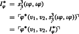
For additional results on the Weak Kleene scheme see Speranski [34], where it is shown that adding a symbol for proper substraction solves the problem.
Where a scheme is supervaluational iff it is given by a rule of the following form: \((\mathbb {N}, E, A)\models _{V}\varphi \) iff for all S⊇E, if Φ(S, E, A) then \((\mathbb {N}, S)\models \varphi \), where Φ is a condition such that for every partial model \((\mathbb {N}, E, A)\) there is an S⊇E with Φ(S, E, A).
This claim is obvious for the Weak Kleene scheme. For the Leitgeb scheme, a counter-example to (S1) can be found in Schindler [29].
Notice that in formulating the T-biconditionals, we have also assumed a Gödelcoding in the metalanguage in order to pick a name for each formula. However, for the derivation (and the results below) it is entirely irrelevant which name is actually chosen, and we could simply pick names at random, with the proviso that no two formulae get the same name assigned.
 and
and  Observe that

References
Beringer, T., & Schindler, T. (2017). A graph-theoretic analysis of the semantic paradoxes. Under review.
Boolos, G., Burgess, J., & Jeffrey, R. (2003). Computability and logic, 4th edn. Cambridge: Cambridge University Press.
Burgess, J.P. (1986). The truth is never simple. Journal of Symbolic Logic, 51, 663–681.
Cain, J., & Damnjanovic, Z. (1991). On the Weak Kleene scheme in Kripke’s theory of truth. Journal of Symbolic Logic, 56, 1452–1468.
Cantini, A. (1989). Notes on formal theories of truth. Zeitschr. f. Math. Logik und Grundlagen d Math, 35, 97–130.
Cantini, A. (1990). A theory of formal truth arithmetically equivalent to ID 1. Journal of Symbolic Logic, 55, 244–259.
Feferman, S. (1991). Reflecting on incompleteness. Journal of Symbolic Logic, 56, 1–49.
Fischer, M., Halbach, V., Kriener, J., & Stern, J. (2015). Axiomatizing semantic theories of truth? Review of Symbolic Logic, 8, 257–278.
Gupta, A. (1982). Truth and paradox. Journal of Philosphical Logic, 11, 1–60.
Halbach, V. (1995). Tarski hierarchies. Erkenntnis, 43, 339–367.
Halbach, V. (1996). Axiomatische Wahrheitstheorien Logica Nova. Berlin: Akademie Verlag.
Halbach, V. (2000). Truth and reduction. Erkenntnis, 53, 97–126.
Halbach, V. (2001). How innocent is deflationism? Synthese, 126, 167–194.
Halbach, V. (2009). Reducing compositional to disquotational truth. Review of Symbolic Logic, 2, 786–798.
Halbach, V. (2011). Axiomatic theories of truth. Cambridge: Cambridge University Press.
Herzberger, H. (1982). Notes on naive semantics. Journal of Philosphical Logic, 11, 61–102.
Horsten, L. (1995). The semantical paradoxes, the neutrality of truth and the neutrality of the minimalist theory of truth. In P. Cortois (Ed.), The many problems of realism, vol. 3 of Studies in the general philosophy of science (pp. 173–187). Tilburg University Press.
Horwich, P. (1998). Truth, 2nd edn. Oxford: Basil Blackwell.
Ketland, J. (1999). Deflationism and Tarski’s paradise. Mind, 108, 69–94.
Kripke, S. (1975). Outline of a theory of truth. Journal of Philosophy, 72, 690–716.
Leitgeb, H. (2005). What truth depends on. Journal of Philosphical Logic, 34, 155–192.
Monk, D.J. (1976). Mathematical logic. New York: Springer.
Moschovakis, Y.N. (1974). Elementary induction on abstract structures. Dover Publications.
Nicolai, C. (2016). Equivalences for truth predicates. Review of Symbolic Logic. forthcoming.
Parsons, C. (1983). Ontology and mathematics. In Mathematics in philosophy (pp. 37–62). Cornell University Press.
Parsons, C. (1983). Sets and classes. In Mathematics in philosophy, (pp. 209–220). Cornell University Press.
Pohlers, W. (2009). Proof theory the first step into impredicativity. Berlin Heidelberg: Springer.
Putnam, H., Boyd, R., & Hensel, G. (1969). A recursion theoretic characterization of the ramified analytical hierarchy. Transactions of the American Mathematical Society, 141(/142), 37–62.
Schindler, T. (2014). Axioms for grounded truth. Review of Symbolic Logic, 7, 73–83.
Schindler, T. (2015). A disquotational theory of truth as strong as Z\(^{-}_{2}\). Journal of Philosophical Logic, 44, 395–410.
Shapiro, S. (1998). Proof and truth: Through thick and thin. Journal of Philosophy, 95, 493–521.
Shoenfield, J.R. (1967). Mathematical logic. Addison-Wesley.
Simpson, S.G. (2009). Subsystems of second order arithmetic, 2nd edn. Cambridge: Cambridge University Press.
Speranski, S.O. (2017). Notes on the computational aspects of Kripke’s theory of truth. Studia Logica, 105, 407–429. https://doi.org/10.1007/s1122501696948.
Tarski, A., Mostowski, A., & Robinson, R. (1953). Undecidable theories. North Holland, Amsterdam.
Visser, A. (1997). An overview of interpretability logic. In Advances in modal logic, (pp. 307–359). Stanford: CSLI Publications.
Visser, A. (2008). Pairs, sets and sequences in first-order theories. Archive for Mathematical Logic, 47, 299–326.
Visser, A. (2009). Cardinal arithmetic in the style of Baron von Münchhausen. Review of Symbolic Logic, 2, 570–589.
Welch, P. (2001). On Gupta-Belnap revision theories of truth, Kripkean fixed points, and the next stable set. Bulletin of Symbolic Logic, 7, 345–360.
Welch, P. (2015). The complexity of the dependence operator. Journal of Philosophical Logic, 44, 337–440.
Acknowledgments
For their help in preparing this paper, I want to thank Timo Beringer, Catrin Campbell-Moore, Volker Halbach, Carlo Nicolai, Stanislav Speranski, and two anonymous referees, one of which spotted a flaw in an old proof of Proposition 14. A special thanks goes to Lavinia Picollo, in particular for her help with Proposition 21 .
Author information
Authors and Affiliations
Corresponding author
Additional information
The author wishes to acknowledge and express his appreciation for the support of the Alexander von Humboldt Foundation and the German Research Foundation (Deutsche Forschungsgemeinschaft, “Reference patterns of paradox”).
Rights and permissions
Open Access This article is distributed under the terms of the Creative Commons Attribution 4.0 International License (http://creativecommons.org/licenses/by/4.0/), which permits unrestricted use, distribution, and reproduction in any medium, provided you give appropriate credit to the original author(s) and the source, provide a link to the Creative Commons license, and indicate if changes were made.
About this article

Cite this article
Schindler, T. Some Notes on Truths and Comprehension. J Philos Logic 47, 449–479 (2018). https://doi.org/10.1007/s10992-017-9434-1
Received:
Accepted:
Published:
Issue Date:
DOI: https://doi.org/10.1007/s10992-017-9434-1