
Abstract
We consider the Cauchy problem for systems of viscous conservation laws. We obtain three different but related stochastic representations of weak solutions of the problem: in terms of solutions to systems of usual backward stochastic differential equations, in terms of solutions to some stochastic backward systems, and in terms of solutions to some forward-backward stochastic differential equations.
1 Introduction
In [19] Pardoux and Peng introduced the notion of nonlinear backward stochastic differential equation (BSDE for short) and soon after Peng [23] and Pardoux and Peng [20] showed that BSDEs provide probabilistic formulas for solutions of systems of semilinear parabolic or elliptic partial differential equations (PDEs) which may be viewed as the nonlinear generalization of the celebrated Feynman–Kac formula. Since then connection between BSDEs and PDEs has been studied intensively by many authors. As a result we know that viscosity or Sobolev space solutions of the Cauchy problem or various boundary problems (e.g. Dirichlet, Neumann or obstacle problem) for single or systems of semilinear PDEs of second order can be represented by solutions of suitable BSDEs (see, e.g., [9, 11, 22, 27, 30]). However, at present satisfactory theory exists only in the case where the right-hand side of the semilinear PDE is Lipschitz-continuous with respect to the solution and its gradient. A lot of effort has been made to relax that condition and prove results for semilinear equations with stronger nonlinearities (see, e.g., [13, 28]). In particular, in a remarkable paper [13] Kobylanski has obtained a nonlinear Feynman–Kac formula for viscosity and Sobolev solutions of a broad class of semilinear parabolic and elliptic PDEs whose right-hand side satisfies some quadratic growth conditions. Let us note, however, that results of [13] concern exclusively single equations. This is due to the fact that in proofs in [13] some comparison theorems for BSDEs associated with equations under consideration are used.
In the present paper we consider weak solutions of the Cauchy problem (for convenience we consider terminal condition) for systems of parabolic perturbations of conservation laws of the form
Here ε>0 is a parameter, \(\varphi=(\varphi^{1},\dots,\varphi^{m}):{\Bbb{R}}^{d}\rightarrow {\Bbb{R}}^{m}\), \(f=(f_{1},\dots,f_{d}):{\Bbb{R}}^{m}\rightarrow {\Bbb{R}}^{m\times d}\) (i.e. f k , k=1,…,d, is a column vector with components \((f^{1}_{k},\dots,f^{m}_{k})\)) are given functions and u is a solution, i.e. \(u=(u^{1},\dots,u^{m}):[0,T]\times {\Bbb{R}}^{d}\rightarrow {\Bbb{R}}^{m}\) is a measurable function satisfying the following system of equations:
in a weak sense (see Sect. 2). Systems of the form (1.1) are important theoretically and in applications. Their importance stems from the fact that in some cases their solutions converge, as ε→0, to solutions of admissible (physically meaningful) solutions of systems of hyperbolic conservation laws (see [8, 17] for results for single equation and [5] for the case m≥1). The systems include, for different choices of f, many basic equations of continuum physics (see, e.g., [8, 17]).
One of the simplest examples of (1.1) is Burgers equation with viscosity which we get putting m=1 and f(x)=|x|2/2, \(x\in {\Bbb{R}}^{d}\). Since Burgers equation can be linearized by the Hopf–Cole transformation, one can write down stochastic representation of its solution by using the classical Feynman–Kac formula and then effectively use the stochastic representation to study properties of the solution. Such approach has been adopted in many papers (see, e.g., [33] and the references therein). The Hopf–Cole transformation can be also applied to the study of multidimensional Burgers equation with data of potential type. The Feynman–Kac representation for solutions of multidimensional Burgers equation with data of non-potential type is given in the recent paper [10].
To our knowledge, the problem of stochastic representation of global solutions (i.e. on fixed interval [0,T]) of general systems of the form (1.1) has not yet been investigated except for the case m=1, which is covered by Kobylanski’s [13] results (see the end of Sect. 3). Multidimensional systems even more general that (1.1) but on a small time interval are investigated in [1, 4] (see Sect. 5).
In the paper we provide three different but related stochastic representations of global solutions of (1.1): in terms of solutions to systems of usual BSDEs, in terms of solutions to some stochastic backward systems and solutions to some forward-backward SDEs. Let us stress, however, that in all cases we assume that there exists a unique bounded weak solution to (1.1). The last problem is difficult except for the case m=1. A nice account of available results on the well-posedness of (1.1) is to be found in [5] (see also Remark 3.3).
In Sect. 3 we prove that if \(\varphi\in L^{2}({\Bbb{R}}^{d})^{m}\cap L^{\infty}({\Bbb{R}}^{d})^{m}\), \(f^{i}\in C^{1}({\Bbb{R}}^{m})^{d}\), i=1,…,d, and there exists a unique bounded continuous weak solution u of (1.1) then for each \((s,x)\in[0,T)\times {\Bbb{R}}^{d}\) the pair of processes (Y s,x,Z s,x) with values in \({\Bbb{R}}^{m}\times {\Bbb{R}}^{m\times d}\) defined by
where
and W=(W 1,…,W d) is a standard d - dimensional Wiener process, is a solution of the following system of BSDEs:

It follows in particular that
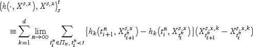
Uniqueness of solutions of (1.3) follows from results of [13] in the case where m=1 and \(f\in C^{2}({\Bbb{R}}^{d})\). We do not know whether uniqueness holds for systems of equations of the form (1.3). However, for systems we are able to prove slightly weaker result. It is not difficult to prove that for each (s,x) and i=1,…,m, k=1,…,d, there exists the quadratic variation \(\langle f^{i}_{k}(Y^{s,x}),X^{s,x,k}\rangle^{T}_{s}\) of processes \(f^{i}_{k}(Y^{s,x})\) and X s,x,k on [s,T] and the second term on the right-hand side of (1.3) equals \(\sum^{d}_{k=1}\langle f^{i}_{k}(Y^{s,x}),X^{s,x,k}\rangle^{T}_{t}\). It follows that the family \(\{(Y^{s,x},Z^{s,x});(s,x)\in[0,T)\times {\Bbb{R}}^{d}\}\) defined by (1.2) is a solution of the system
In Sect. 4 we consider general systems \(\{(Y^{s,x},Z^{s,x}); (s,x)\in[0,T)\times {\Bbb{R}}^{d}\}\) of the form (1.5) with u defined by the first component \(\{Y^{s,x},(s,x)\in[0,T)\times {\Bbb{R}}^{d}\}\) of the system via (1.4). From (1.4) it follows that u is bounded. Since one can show that for any bounded measurable u the quadratic variation process \(t\mapsto\langle f^{i}_{k}\circ u(\cdot,X^{s,x}),X^{s,x,k}\rangle^{t}_{s}\) exists and is a 0-quadratic variation process, it is natural to consider systems (1.5) such that for each \((s,x)\in[0,T)\times {\Bbb{R}}^{d}\) the process Y s,x is a Dirichlet process, i.e. admits the decomposition into a continuous process of 0-quadratic variation and a continuous square-integrable martingale. Roughly speaking, our uniqueness result says that there is at most one family \(\{(Y^{s,x},Z^{s,x}); (s,x)\in[0,T)\times {\Bbb{R}}^{d}\}\) such that Y s,x is a Dirichlet process on [s,T] and (1.5) is satisfied for every \((s,x)\in[0,T)\times {\Bbb{R}}^{d}\) with u defined by (1.4).
In Sect. 5 we first consider single equation of conservation law. We give representation of its solution u by means of weak solutions of some forward-backward SDEs, which in turn implies that u is a solution of the system
Following [1] we also show that using ideas from [31] one can generalize representation of the form (1.6) to systems of conservation laws.
The case where m=1 and φ,f′ are Lipschitz-continuous existence of a unique solution of (1.6) follows from results proved in [21]. Systems of the form (1.6) with regular φ are investigated in [1, 4] by methods completely different from those adopted in the present paper. In [1, 4] it is proved that there is a unique solution of (1.6) on [0,T 0] for some small T 0>0.
In the paper we consider exclusively equations of conservation laws, but at the expense of minor technical complications our results can be extended to equations of balance laws of the form
where \(g:{\Bbb{R}}^{m}\rightarrow {\Bbb{R}}^{m}\) is a Lipschitz-continuous function.
Stochastic representation of solutions to Burgers equation allows one to study efficiently various properties of these solutions (see, e.g., [33]). We think that the representations obtained in the paper lead to new insights into the structure of solutions of more general equations (1.1) and (1.7) and as in the case of Burgers equation will be useful in the investigation of their properties. Our representation may also serve as the starting point for the construction of numerical algorithms for (1.1), (1.7). To our knowledge, at present deterministic algorithms based on representation of solutions in terms of BSDEs are known only in the case where the right-hand side of the equation is Lipschitz-continuous with respect to the solution and its gradient (see, e.g., [6]). Another kind of algorithms based on probabilistic representation of solutions to semilinear parabolic equations is to be found in [18].
Notation
\(Q_{T}=(0,T)\times {\Bbb{R}}^{d}\), ∥z∥2=Tr(zz ∗) for \(z\in {\Bbb{R}}^{m\times d}\), ∂/∂x i is the partial derivative in the distribution sense. L p(D) (resp. L ∞(D)) is the usual Banach space of measurable functions on D that are p-integrable (resp. essentially bounded); \(W^{1}_{2}({\Bbb{R}}^{d})\) (resp. \(W^{0,1}_{2}(Q_{T})\)) is the usual Sobolev space of all elements u of \(L^{2}({\Bbb{R}}^{d})\) (resp. L 2(Q T )) having derivatives ∂u/∂x i in \(L^{2}({\Bbb{R}}^{d})\) (resp. L 2(Q T )); \(W^{1,1}_{2}(Q_{T})\) is the space of elements of L 2(Q T ) having derivatives ∂u/∂x i and time derivatives from L 2(Q T ), and \(\mathcal {W}(Q_{T})=\{u\in W^{0,1}_{2}(Q_{T}):\partial u/\partial t\in L^{2}(0,T;W^{-1}_{2}({\Bbb{R}}^{d}))\}\), where \(W^{-1}_{2}({\Bbb{R}}^{d})\) is the space dual to \(W^{1}_{2}({\Bbb{R}}^{d})\). By ∥⋅∥2 we denote the norm in \(L^{2}({\Bbb{R}}^{d})\) and by ∥⋅∥2;0,T the norm in L 2(Q T ).
2 Preliminary Results
Let W be a standard d-dimensional Wiener process defined on some probability space (\(\varOmega ,\mathcal {F},P\)). For fixed 0≤s<T set
Then \(\{\hat{W}_{t}-\hat{W}_{0};t\in[0,T]\}\) is a standard d-dimensional Wiener process and, by Exercise 3.18 in Chap. IV of [24], {B s,t ;t∈[0,T]} is a standard d-dimensional Wiener process with respect to the filtration \(\{\mathcal {G}^{s}_{t}=(\mathcal {F}^{\hat{W}_{\cdot}-\hat{W}_{0}}_{t}\vee\sigma(\hat{W}_{0}))_{+}\}_{t\in[0,T]}\). Write
By (2.1),
Thus,
where
Let us note that the decomposition (2.2) may be viewed as a very special case of the strict Fukushima–Lyons–Zheng decomposition of diffusions corresponding to divergence form operators (see [25, 26]).
Let \(h=(h_{1},\dots,h_{d}):[s,T]\times {\Bbb{R}}^{d}\rightarrow {\Bbb{R}}^{d}\). Following [29] let us consider the family of integrals
defined by

where \(\bar{h}(t,x)=h(T+s-t,x)\), \((t,x)\in[0,T]\times {\Bbb{R}}^{d}\), \(\bar{X}^{s,x}_{t}=X^{s,x}_{T+s-t}\), t∈[s,T].
Let \(\mathcal {F}^{s}_{t}\) denote the σ-algebra σ(W u −W s ,u∈[s,t]) augmented by P-null subsets of \(\mathcal {F}^{s}_{T}\). A continuous \(\{\mathcal {F}^{s}_{t}\}\)-adapted process A on [0,T] is called a 0-quadratic variation process if
in probability P as n→0 for any sequence \(\{\varPi _{n}=\{s=t^{n}_{0}<t^{n}_{1}<\dots<t^{n}_{k(n)}=T\}\}\) of partitions of [s,T] such that \(\max_{0\le i\le k(n)}(t^{n}_{i+1}-t^{n}_{i})\rightarrow0\).
Proposition 2.1
Let \(h:[s,T]\times {\Bbb{R}}^{d}\rightarrow {\Bbb{R}}^{d}\) be a bounded measurable function. Then for each \(x\in {\Bbb{R}}^{d}\),
-
(i)
H s,x(h) is a 0-quadratic variation process on [s,T].
-
(ii)
The quadratic covariation
exists as limit in probability P and
$$H^{s,x}_t=\bigl\langle h\bigl(\cdot,X^{s,x}\bigr),X^{s,x}\bigr\rangle^t_s,\quad t\in[s,T].$$ -
(iii)
If, in addition, \(h\in W^{0,1}_{2}(Q_{T})^{d}\) and \(E\int^{T}_{s}|\nabla h(\theta,X^{s,x}_{\theta})|^{2}\,d\theta<\infty\), then
$$ \varepsilon^2\int^t_s\operatorname {div}h\bigl(\theta,X^{s,x}_{\theta}\bigr)\,d\theta =H^{s,x}_t(h), \quad t\in[s,T],\ P\mbox{-}a.s.$$(2.3)

Proof
Assertion (i) follows from the proof of [29, Lemma 3.2(ii)] while (iii) is the special case of [29, Lemma 3.1]. Assertion (ii) follows easily from the equality

where \(\varPi ^{*}_{n}=\{T+s-t^{n}_{i}:t^{n}_{i}\in \varPi _{n}\}\), and the fact that V s,⋅ is a process of finite variation on [s,T]. □
Identity (2.3) will play the key role in Sect. 4. Integrating (2.3) gives
Notice that one can obtain (2.4) without referring to (2.3) by using the integration by parts formula.
Let 〈⋅,⋅〉 denote the duality between \(W^{1}_{2}({\Bbb{R}}^{d})\) and its dual space \(W^{-1}_{2}({\Bbb{R}}^{d})\). Let us recall that \(u\in \mathcal {W}(Q_{T})^{m}\) is a weak solution of (1.1) if u(T)=φ and
for almost all s∈[0,T] and all \(\psi\in W^{1}_{2}({\Bbb{R}}^{d})\) (see, e.g., [17, Chap. 2]). Equivalently, u is a weak solution of (1.1) if

for all \(\eta=(\eta^{1},\dots,\eta^{m})\in W^{1,1}_{2}(Q_{T})\) (see [14, p. 572]).
3 Backward SDEs
Let \(\mathcal {L}_{2}(x,s,T)^{m}\) denote the space of functions \(u:[s,T]\times {\Bbb{R}}^{d}\rightarrow {\Bbb{R}}^{m}\) having a finite norm \(\|u\|^{2}_{\mathcal {L}_{2}(x,s,T)^{m}}=\int^{T}_{s}\int_{{\Bbb{R}}^{d}}|u(t,y)|^{2}p_{t-s}(y-x)\,dt\,dy\), where p t is the probability density of W t , and let \(\mathcal {W}_{2}(x,s,T)^{m}\) denote the subspace of \(\mathcal {L}_{2}(x,s,T)^{m}\) consisting of all elements such that \(\|u\|^{2}_{\mathcal {W}_{2}(x,s,T)^{m}}=\|u\|^{2}_{\mathcal {L}_{2}(x,s,T)^{m}}+\|\nabla u\|^{2}_{\mathcal {L}_{2}(x,s,T)^{m}}<\infty\).
Proposition 3.1
Assume that \(\varphi\in L^{2}({\Bbb{R}}^{d})^{m}\cap L^{\infty}({\Bbb{R}}^{d})^{m}\), \(f^{i}\in C^{1}({\Bbb{R}}^{m})^{d}\), i=1,…,m, and \(v\in W^{0,1}_{2}(Q_{T})^{m}\cap L^{\infty}(Q_{T})^{m}\). Then there exists a unique weak solution \(u\in \mathcal {W}(Q_{T})^{m}\cap L^{\infty}(Q_{T})^{m}\) of the problem
Moreover, u has a version which is continuous on \([0,T)\times {\Bbb{R}}^{d}\). If, in addition, \(v\in W^{0,1}_{2}(Q_{T})^{m}\) and \(v\in \mathcal {W}_{2}(x,s,T)^{m}\) for some \((s,x)\in[0,T)\times {\Bbb{R}}^{d}\), then \(u\in \mathcal {W}_{2}(x,s,T)^{m}\) and the pair
is a solution of the system of linear BSDEs

Proof
Since v∈L ∞(Q T )m, we may and will assume that f has compact support. But then f i(v)∈L 2(Q T )d∩L ∞(Q T )d, i=1,…,m, so there is a unique weak solution \(u\in \mathcal {W}_{T}(Q_{T})^{m}\) of (3.1) (see, e.g., [15, Theorem 3.1.2] or [14, p. 574]) which has bounded continuous version on \([0,T)\times {\Bbb{R}}^{d}\) (see, e.g., [3]). Thus, what is left is to show that \(u\in \mathcal {W}_{2}(x,s,T)^{m}\) and (3.2) is satisfied if \(v\in W^{0,1}_{2}(Q_{T})^{m}\cap \mathcal {W}_{2}(x,s,T)^{m}\). Using mollification one can construct sequences {φ n }, {g n } of bounded smooth functions such that \(\varphi^{i}_{n}\rightarrow\varphi^{i}\) in \(L^{2}({\Bbb{R}}^{d})\) and \(g^{i}_{n,k}\rightarrow f^{i}_{k}(v)\) in \(W^{0,1}_{2}(Q_{T})\) as n→∞, and ∥φ n ∥∞≤∥φ∥∞, ∥g n ∥∞≤∥f∘v∥∞. Let u n be a classical solution of the Cauchy problem
By Itô’s formula, the pair \((Y^{n},Z^{n}_{t}=(Z^{n,1},\dots,Z^{n,m}))\) defined by \(Y^{n,i}_{t}=u_{n}^{i}(t,X^{s,x}_{t})\), \(Z^{n,i}_{t}=\varepsilon\nabla u^{i}_{n}(t,X^{s,x}_{t})\), t∈[s,T], i=1,…,m, is a solution of the system of BSDEs
By the above and (2.4),
Hence
where
Using once again Itô’s formula we see that
Since \(u^{i}_{n}\operatorname {div}g^{i}_{n}=\operatorname {div}(u^{i}_{n}g^{i}_{n})-\sum^{d}_{k=1}g^{i}_{n,k}(\partial u^{i}_{n}/\partial x_{k})\), it follows from (2.4) that

which when combined with (3.4) shows that \(\sup_{n\ge1}E\int^{T}_{s}\|Z^{n}_{t}\|^{2}\,dt<\infty\). Thus, {u n } is bounded in \(\mathcal {W}_{2}(x,s,T)^{m}\) and hence is weakly relatively compact. This shows that \(u\in \mathcal {W}_{2}(s,x,T)^{m}\), because by the well-known convergence results, u n →u in \(W^{0,1}_{2}(Q_{T})^{m}\). Since (3.4) holds true for all \((s,x)\in[0,T]\times {\Bbb{R}}^{d}\), the functions u n are uniformly bounded and hence, by Nash’s continuity theorem, equicontinuous. Therefore u n →u uniformly in compact subsets of \([0,T)\times {\Bbb{R}}^{d}\). Using this and the fact that \(\operatorname {div}g^{i}_{n}\rightarrow \operatorname {div}f^{i}(v)\), \(\nabla u^{i}_{n}\rightarrow\nabla u^{i}\) in L 2(Q T ) for i=1,…,m, we conclude from (3.3) that the pair (Y s,x,Z s,x) satisfies (3.2) on [s+δ,T] for every δ∈(0,T−s). Since \(f^{i}\circ v\in \mathcal {L}_{2}(x,s,T)^{m}\) if \(v\in \mathcal {W}_{2}(x,s,T)^{m}\) and we already know that \(\nabla u\in \mathcal {L}_{2}(x,s,T)\), (3.2) is satisfied on the whole interval [s,T]. □
We are ready to prove existence of solutions of BSDE (1.3) under the following basic hypothesis:
-
(H)
There exists a unique weak solution \(v\in \mathcal {W}(Q_{T})^{m}\cap L^{\infty}(Q_{T})^{m}\) to the Cauchy problem (1.1).
The problem of existence and uniqueness of global weak solutions to general systems of the form (1.1) is subtle and difficult except for the case m=1. A nice presentation of recent results on the topic is given in [5]. Some sufficient conditions for (H) to hold are given in Remark 3.3.
In what follows by \(\mathcal {H}^{2}(s,T)^{m}\) we denote the space of all \(\{\mathcal {F}^{s}_{t}\}_{t\in[s,T]}\)-progressively measurable m-dimensional processes ξ on [s,T] such that \(E\int^{T}_{s}|\xi_{t}|^{2}\,dt<\infty\) and by \(\mathcal {H}^{\infty}(s,T)^{m}\) the subspace of \(\mathcal {H}^{2}(s,T)^{m}\) consisting of all processes that are P-a.s. bounded.
Theorem 3.2
Assume that \(\varphi\in L^{2}({\Bbb{R}}^{d})^{m}\cap L^{\infty}({\Bbb{R}}^{d})^{m}\), \(f^{i}\in C^{1}({\Bbb{R}}^{m})^{d}\), i=1,…,d, and (H) is satisfied. Then v has a version u which is continuous on \([0,T)\times {\Bbb{R}}^{d}\) and for each \((s,x)\in[0,T)\times {\Bbb{R}}^{d}\) the pair \((Y^{s,x},Z^{s,x})\in \mathcal {H}^{\infty}(s,T)^{m}\times \mathcal {H}^{2}(s,T)^{md}\) defined by (1.2) is a solution of BSDE (1.3).
Proof
Let M=∥v∥∞ and let g=(g 1,…,g m), g i=ζf i, i=1,…,m, where \(\zeta:{\Bbb{R}}^{d}\rightarrow[0,1]\) is a smooth function with compact support such that ζ(y)=1 if |y|≤M+1. Suppose that the pair \((Y^{s,x}_{t},Z^{s,x}_{t})=(v(t,X^{s,x}_{t}),\varepsilon\nabla v(t,X^{s,x}_{t}))\), t∈[s,T], is a solution of (1.1) with f replaced by g. Since \(\frac{\partial f^{i}_{k}}{\partial u^{j}}(Y_{t})=\frac{\partial g^{i}_{k}}{\partial u^{j}}(Y_{t})\), t∈[s,T], it follows that (Y s,x,Z s,x) solves the original equation (1.3). Therefore we may and will assume that f is globally Lipschitz-continuous and bounded, i.e. there exist constants K,L>0 such that
Let λ>0 and let V λ denote the space \(V=W^{0,1}_{2}(Q_{T})^{m}\cap C([0,T];L^{2}({\Bbb{R}}^{d})^{m})\) equipped with the norm
where u λ (t,x)=e λt/2 u(t,x). Since ∥⋅∥ λ is equivalent to the usual norm in V, V λ is a Banach space. Define the mapping Φ:V λ →V λ by putting Φ(v) to be the solution of (3.1). We shall show that Φ is a contraction for all sufficiently large λ. Let v 1,v 2 be two elements of V λ and let u 1=Φ(v 1),u 2=Φ(v 2), u=u 1−u 2. Then for any \(\psi\in W^{0,1}_{2}(Q_{T})\) and i=1,…,m,
for a.e. t∈(0,T). Since 2e λt u i ∂u i/∂t=∂(e λt(u i)2)/∂t−λe λt(u i)2, putting ψ(x)=e λt u i(t,x) and integrating over the interval (t,T)⊂(s,T) we obtain

Hence

for i=1,…,m, which shows that Φ is a contraction if λ>8dL 2 ε −2. Set u 0=0, u n =Φ(u n−1), \(n\in {\Bbb{N}}\). By the Banach principle, {u n } converges in V λ to the unique fixed point of Φ, i.e. to the unique weak solution v of (1.1).
Set
By Proposition 3.1,
As in the proof of (3.4), from (3.5) we deduce that |u n (s,x)|≤∥φ∥∞+Kε −1 ER 0,T . Since (3.5) holds true for every \((s,x)\in[0,T)\times {\Bbb{R}}^{d}\), we see that the functions u n are bounded uniformly in \(n\in {\Bbb{N}}\), and hence, by Nash’s continuity theorem, equicontinuous. Therefore we may apply the Ascoli–Arzela theorem and choose a sequence (still denoted by {n}) such that {u n } converges uniformly in compact subsets of \([0,T)\times {\Bbb{R}}^{d}\) to some bounded \(u\in C([0,T)\times {\Bbb{R}}^{d})^{m}\). Of course, u is a version of v. Set \(Y^{s,x}_{t}=u(t,X^{s,x}_{t})\), t∈[s,T]. Since \(Y^{n}_{t}\rightarrow Y^{s,x}_{t}\) a.s. for t∈[s,T] and Y n are bounded uniformly in n, applying the Lebesgue dominated convergence theorems gives
Since for any \(n,m\in {\Bbb{N}}\),

applying Itô’s formula and using (2.4) gives

for some C>0 not depending on n,m, which when combined with (3.6) shows that {Z n} is a Cauchy sequence in \(\mathcal {H}^{2}(s,T)^{m}\). On the other hand, since u n →u in V, \(E\int^{T}_{s+\delta}\|Z^{n}_{t}-\varepsilon\nabla u(t,X^{s,x}_{t})\|^{2}\,dt\rightarrow0\) for every δ∈(0,T−s). Thus, if we set \(Z^{s,x}_{t}=\varepsilon\nabla u(t,X^{s,x}_{t})\), t∈[s,T], then
Letting n→∞ in (3.5) and using (3.6), (3.7) shows that (Y s,x,Z s,x) solves (1.3). □
Remark 3.3
(i) In case m=1 existence of a unique weak solution \(u\in \mathcal {W}(Q_{T})\cap L^{\infty}(Q_{T})\) to (1.1) is well known (see, e.g., [17, Theorem 2.9]). It is known also that ∥u∥∞≤∥φ∥∞. Observe that the above results follows from the proof of Theorem 3.2. Indeed, the function u constructed in the proof is a solution of the problem (1.1) with f replaced by g, so we only have to show that ∥u∥∞≤∥φ∥∞. The last inequality may be proved probabilistically as follows. Set M=∥φ∥∞ and denote by L={L t ;t∈[s,T]} the local time at zero of the semimartingale Y s,x−M. By the Tanaka–Meyer formula, we have
Hence

Since \((Y^{s,x}_{T}-M)^{+}=0\), it follows from the above that

for some C depending on ε,L. Putting λ=C we see that \(E|(Y^{s,x}_{s}-M)^{+}|^{2}=0\), which implies that ∥u∥∞≤M.
(ii) Consider now the system (1.1) in space dimension d=1. Then (H) is satisfied if \(\varphi\in L^{\infty}({\Bbb{R}})\cap W^{1}_{2}({\Bbb{R}})\), \(f\in C^{1}({\Bbb{R}})\) and f is Lipschitz-continuous with some constant L>0. To prove this we only have to show that the solution u constructed in the proof of Theorem 3.2 is bounded. Observe also that without loss of generality we may and will assume that f(0)=0 (if necessary, we can replace f by \(\tilde{f}(y)=f(y)-f(0)\)).
Applying Itô’s formula to (3.5) and taking expectation gives

for i=1,…,m. Integrating the above equality with respect to x we get

Since u 0=0, we deduce from the above that

for s∈[0,T]. Put v n =∂u n /∂x. ψ=∂φ/∂x. Since
we have
From this it follows that for i=1,…,m,

By the above and (3.8) there is c not depending on n such that
for each i=1,…,m. Since, by the imbedding theorem, there is c′>0 not depending on n such that \(\|u_{n}(s,\cdot)\|_{\infty}\le c'\|u_{n}(s,\cdot)\|_{W^{1}_{2}({\Bbb{R}})}\) for s∈[0,T), it follows from (3.8), (3.9) that \(\sup_{n\ge0}\|u_{n}\|_{\infty}\le C\|\varphi\|_{W^{1}_{2}({\Bbb{R}})}\), and hence that \(\|u\|_{\infty}\le C\|\varphi\|_{W^{1}_{2}({\Bbb{R}})}\).
Note that the above proof is a modification of the proof given in Exercise 10 in Sect. 15.1 of [32] (the proof given in [32] shows in fact that the assumption that f is Lipschitz-continuous can be weakened).
(iii) In the general case (m≥1,d≥1) existence and uniqueness of global bounded weak solutions to (1.1) is known to hold if the system is strictly hyperbolic and the total variation and the supremum norm of the final condition φ are sufficiently small (see [5] and the references therein).
Let us note that in case of scalar conservation laws, i.e. if m=1, existence of solutions of (1.3) follows from [13, Theorem 2.3]. Uniqueness holds under some further restrictions on f.
Theorem 3.4
Let m=1. Then under assumptions of Theorem 3.2, if moreover \(f\in C^{2}({\Bbb{R}})^{d}\), for each \((s,x)\in[0,T)\times {\Bbb{R}}^{d}\) there exists at most one solution of BSDE (1.3) in the class \(H^{\infty}(s,T)\times \mathcal {H}^{2}(s,T)^{d}\).
Proof
The proof follows from [13, Theorem 2.6], because the function \(F(y,z)=\sum^{d}_{k=1}f'_{k}(y)z_{k}\), \(y\in {\Bbb{R}}\), \(z\in {\Bbb{R}}^{d}\), satisfies hypotheses (H2), (H3) of [13]. □
Remark 3.5
(i) Let \((\tilde{\varOmega },\tilde{\mathcal {F}},\tilde{P})\) be a complete probability space equipped with some filtration \(\{\tilde{\mathcal {F}}^{s}_{t}\}_{t\in[s,T]}\) satisfying the usual conditions, and let \(\tilde{X}^{s,x}_{t}=x+\varepsilon\tilde{W}_{t}\), t∈[s,T], where \(\tilde{W}\) is an \(\{\tilde{\mathcal {F}}^{s}_{t}\}\)-Wiener process on \((\tilde{\varOmega },\tilde{\mathcal {F}},\tilde{P})\) starting at time s from 0. The proof of Theorem 3.2 shows that the pair
where u is a continuous weak solution of (1.1), is a solution on \((\tilde{\varOmega },\tilde{\mathcal {F}},\tilde{P})\) of the system

(to see this it suffices to observe that in the proof of (3.2), which is used to prove (3.5), and in arguments following (3.5) we do not use the fact that the underlying filtration is generated by a Wiener process).
(ii) Similarly, since in the proof of the comparison principle [13, Theorem 2.6] the fact that the solutions under consideration are adapted to the natural filtration generated by a Wiener process is not used, in case m=1, \(f\in C^{2}({\Bbb{R}})^{d}\), the pair (3.10) is a unique \(\{\tilde{\mathcal {F}}^{s}_{t}\}\)-adapted solution of (3.11) on \((\tilde{\varOmega },\tilde{\mathcal {F}},\tilde{P})\) (with the Wiener process \(\tilde{W}\)) in the class \(H^{\infty}(s,T)\times \mathcal {H}^{2}(s,T)^{d}\). Thus, if m=1 and \(f\in C^{2}({\Bbb{R}})^{d}\), then the solution of (1.3) is weakly unique (for the definition of weak uniqueness see [16] and Sect. 5).
4 Stochastic Backward Systems
From Theorem 3.2 and (2.3) it follows that under hypothesis (H) the family \(\{(Y^{s,x},Z^{s,x});(s,x)\in[0,T)\times {\Bbb{R}}^{d}\}\) is a solution, in the class \(\mathcal {H}^{\infty}\times \mathcal {H}^{2}\), of the stochastic backward system associated with φ,f in the sense that for every \((s,x)\in[0,T)\times {\Bbb{R}}^{d}\) the pair \((Y^{s,x},Z^{s,x})\in \mathcal {H}^{\infty}(s,T)\times \mathcal {H}^{2}(s,T)\) is a solution of the system
Let us point out that from the second equation in (4.1) it follows that \(u(s,x)=Y^{s,x}_{s}\) a.s., so the function u appearing in (4.1) is determined by the first component \(\{Y^{s,x}; (s,x)\in[0,T)\times {\Bbb{R}}^{d}\}\) of the system.
We will say that system (4.1) has a unique solution in \(\mathcal {H}^{\infty}\times \mathcal {H}^{2}\) if \({}^{1}Y^{s,x}_{t}={}^{2}Y^{s,x}_{t}\), t∈[s,T], a.s. and \(E\int^{T}_{s}|{}^{1}Z^{s,x}_{t}-{}^{2}Z^{s,x}_{t}|^{2}\,dt=0\) for every \((s,x)\in[0,T)\times {\Bbb{R}}^{d}\) for any system \(\{({}^{k}Y^{s,x},{}^{k}Z^{s,x});(s,x)\in[0,T)\times {\Bbb{R}}^{d}\}\in \mathcal {H}^{\infty}\times \mathcal {H}^{2}\), k=1,2, associated with φ,f. Notice also that from the definition of a solution of the stochastic system and remark preceding formula (2.3) it follows that if f is locally bounded then for each \((s,x)\in[0,T)\times {\Bbb{R}}^{d}\) the process Y s,x is a Dirichlet process in the sense of Föllmer, i.e. admits a (unique) decomposition into a continuous square-integrable martingale and a continuous process of 0-quadratic variation.
Theorem 4.1
Under assumptions of Theorem 3.2 the stochastic system (4.1) has a unique solution in \(\mathcal {H}^{\infty}\times \mathcal {H}^{2}\).
Proof
Suppose that \(\{({}^{k}Y^{s,x},{}^{k}Z^{s,x}),(s,x)\in[0,T)\times {\Bbb{R}}^{d}\}\), k=1,2, are two solutions of (4.1). Set \({}^{k}Y^{s,x}_{s}=u_{k}(s,x)\) and for fixed s,x write Y=1 Y s,x−2 Y s,x, Z=1 Z s,x−2 Z s,x. By Itô’s formula for Dirichlet processes (see [7, Lemma 2.5]),

where \(h^{i}=(h^{i}_{1},\dots,h^{i}_{d})\), \(h^{i}_{k}=f^{i}_{k}(u_{1})-f^{i}_{k}(u_{2})\). Let \(\{\varPi ^{n}=\{s=t^{n}_{0}<\dots<t^{n}_{n}=T\}\}\) be a sequence of partitions of [s,T] such that \(\max_{0\le j<n}(t^{n}_{j+1}-t^{n}_{j})\rightarrow0\) as n→∞ and let \(s^{n}_{j}=T+s-t^{n}_{n-j}\). Since the integral \(\int^{T}_{s}e^{\lambda t}Y^{i}_{t}\,dH^{s,x}_{t}(h^{i})\) exists as limit in probability of Riemann sums and t↦e λt is of finite variation, for k=1,…,d we have

(here \(\bar{Y}^{i}_{t}=Y^{i}_{T+s-t}\)). The mutual quadratic variation above can be estimated by
Since Y i is a Dirichlet process with the martingale part \(\sum^{d}_{k=1}\int^{\cdot}_{s}Z^{ik}_{\theta}\,dW^{k}_{\theta}\), it follows that
Moreover,

By the above,

which when combined with (4.2) gives

Write u=u 1−u 2, \(g^{i}_{k}=u^{i}h^{i}_{k}\). By elementary calculations, for every t∈(s,T] we have

Therefore putting λ=Lε −2 and integrating both sides of (4.3) with respect to the space variables, we conclude that \(\|u^{i}(s,\cdot)\|^{2}_{2}=0\) for i=1,…,m. Thus, u(s,⋅)=0 a.e. on \({\Bbb{R}}^{d}\) for every s∈[0,T]. Since for fixed \((s,x)\in[0,T)\times {\Bbb{R}}^{d}\) we have

it follows that
Consequently, \(Y_{t}=-\int^{T}_{t}Z_{\theta}\,dW_{\theta}\), t∈[s,T], and hence Y=0, Z=0, which proves the theorem. □
5 Forward-Backward BSDEs
It is worth pointing out that in case m=1 the continuous weak solution u of (1.1) may be represented by weak solutions of forward-backward stochastic differential equation (FBSDE)
associated with (1.1). Before proving the representation, we give definitions of weak solution and weak uniqueness for the above FBSDE.
Following [2, 16], by a weak solution of FBSDE (5.1) we mean a triple \((\tilde{\varOmega },\tilde{\mathcal {F}},\tilde{P})\), \((\tilde{W},\{\tilde{\mathcal {F}}_{t}\}_{t\in[s,T]})\), \((\tilde{X}^{s,x},\tilde{Y}^{s,x},\tilde{Z}^{s,x})\), where \((\tilde{\varOmega },\tilde{\mathcal {F}},\tilde{P})\) is a complete probability space, \(\{\tilde{\mathcal {F}}_{t}\}_{t\in[s,T]}\) is a filtration of sub-σ-fields of \(\tilde{\mathcal {F}}\) satisfying the usual conditions, \(\tilde{W}\) is an \(\{\tilde{\mathcal {F}}^{s}_{t}\}\)-Wiener process on \((\tilde{\varOmega },\tilde{\mathcal {F}},\tilde{P})\) starting at time s from 0, the processes \(\tilde{X}^{s,x},\tilde{Y}^{s,x}\) are continuous, all processes \(\tilde{X}^{s,x},\tilde{Y}^{s,x},\tilde{Z}^{s,x}\) are \(\{\tilde{\mathcal {F}}_{t}\}_{t\in[s,T]}\)-adapted and (5.1) is satisfied \(\tilde{P}\)-a.s.
If, in addition, \(\tilde{Y}^{s,x}\) is \(\tilde{P}\)-a.s. bounded on [s,T] and \(E_{\tilde{P}}\int^{T}_{s}(|X^{s,x}_{t}|^{2}+|Z^{s,x}_{t}|^{2})\,dt<\infty\), we shall say that the weak solution is of class \(\mathcal {H}^{2,\infty,2}(s,T)\).
We say that weak uniqueness holds for (5.1) in the class \(\mathcal {H}^{2,\infty,2}(s,T)\) if for any two weak solutions \((\tilde{\varOmega }^{1},\tilde{\mathcal {F}}^{1},\tilde{P}^{1})\), \((\tilde{W}^{1},\{\tilde{\mathcal {F}}^{i}_{t}\})\), \((\tilde{X}^{1},\tilde{Y}^{1},\tilde{Z}^{1})\) and \((\tilde{\varOmega }^{2},\tilde{\mathcal {F}}^{2},\tilde{P}^{2})\), \((\tilde{W}^{2},\{\tilde{\mathcal {F}}^{2}_{t}\})\), \((\tilde{X}^{2},\tilde{Y}^{2},\tilde{Z}^{2})\) of (5.1) such that \((\tilde{X}^{i},\tilde{Y}^{i},\tilde{Z}^{i})\in \mathcal {H}^{2,\infty,2}(s,T)\) the finite-dimensional distributions of \((\tilde{X}^{1},\tilde{Y}^{1},\tilde{Z}^{1})\) under \(\tilde{P}^{1}\) are equal to the finite-dimensional distributions of \((\tilde{X}^{2},\tilde{Y}^{2},\tilde{Z}^{2})\) under \(\tilde{P}^{2}\).
Theorem 5.1
Let m=1 and let φ,f satisfy the assumptions of Theorem 3.2. Then for each \((s,x)\in[0,T)\times {\Bbb{R}}^{d}\) there exists a weak solution of FBSDE (5.1) in the class \(\mathcal {H}^{2,\infty,2}(s,T)\). If, in addition, \(f\in C^{2}({\Bbb{R}}^{d})\), then weak uniqueness holds for (5.1) in the class \(\mathcal {H}^{2,\infty,2}(s,T)\), and if \((\tilde{X}^{s,x},\tilde{Y}^{s,x},\tilde{Z}^{s,x})\in \mathcal {H}^{2,\infty,2}(s,T)\) is a solution of (5.1) on some stochastic basis, then
where u is a continuous weak solution of (1.1).
Proof
Existence of weak solutions follows immediately from Theorem 3.2 by Girsanov’s theorem. Indeed, let (Y s,x,Z s,x) be a solution of (1.3) for some \((s,x)\in[0,T)\times {\Bbb{R}}^{d}\). Let
and let \(\tilde{P}\) be a measure on \(\mathcal {F}^{s}_{T}\) such that \(d\tilde{P}/dP=N^{s,x}_{T}\). Since under \(\tilde{P}\) the process
is an \(\{\mathcal {F}^{s}_{t}\}\)-standard Wiener process starting at time s from 0, it follows from (1.3) with m=1 that (X s,x,Y s,x,Z s,x), \((\tilde{W},\{\mathcal {F}^{s}_{t}\})\) is a solution of (5.1) on \((\varOmega ,\mathcal {F},\tilde{P})\).
To prove uniqueness, let us fix (s,x) and suppose that \((\tilde{X}^{i},\tilde{Y}^{i},\tilde{Z}^{i})\in \mathcal {H}^{2,\infty,2}(s,T)\), \((\tilde{W}^{i},\{\tilde{\mathcal {F}}^{i}_{t}\})\), i=1,2, are two solutions of (5.1) defined on spaces \((\tilde{\varOmega }^{i},\tilde{\mathcal {F}}^{i},\tilde{P}^{i})\), i=1,2, respectively. Let
Since M i is an \(\{\tilde{\mathcal {F}}^{i}_{t}\}\)-martingale on [s,T] under \(\tilde{P}^{i}\), applying Girsanov’s theorem we see that under Q i given by \((dQ^{i}/d\tilde{P}^{i})=M^{i}_{T}\) the process
is an \(\{\tilde{\mathcal {F}}^{i}_{t}\}\)-standard Wiener process on \((\tilde{\varOmega }^{i},\tilde{\mathcal {F}}^{i},Q^{i})\) starting at time s from 0. Therefore \((\tilde{X}^{i},\tilde{Y}^{i},\tilde{Z}^{i})\), \((\hat{W}^{i},\{\tilde{\mathcal {F}}^{i}_{t}\})\) is a solution of the BSDE
on \((\tilde{\varOmega }^{i},\tilde{\mathcal {F}}^{i},Q^{i})\). By Remark 3.5,
where u is a continuous weak solution of (1.1). On the other hand, since the distributions of \(\tilde{X}^{1}\) under Q 1 and \(\tilde{X}^{2}\) under Q 2 are equal and for i=1,2 the density \(1/M^{i}_{T}\) of \(\tilde{P}^{i}\) with respect to Q i may be expressed as a functional of \((\tilde{X}^{i},\tilde{Y}^{i})\), equality (5.5) implies that the finite-dimensional distributions of \(\tilde{X}^{1}\) under \(\tilde{P}^{1}\) and \(\tilde{X}^{2}\) under \(\tilde{P}^{2}\) are equal, which together with (5.5) completes the proof of weak uniqueness and (5.2). □
Notice that existence of weak solutions of (5.1) may be proved without referring to Girsanov’s theorem. Indeed, we can first find a unique weak solution \((\tilde{\varOmega },\tilde{\mathcal {F}},\tilde{P})\), \((\tilde{W},\{\tilde{\mathcal {F}}_{t}\})\), X s,x of the Itô equation
where u is a continuous weak solution of (1.1), and then as in the proof of Proposition 3.1 show that the pair \((\tilde{Y}^{s,x}_{t},\tilde{Z}^{s,x}_{t})=(\tilde{u}(t,\tilde{X}^{s,x}_{t}),\varepsilon\nabla \tilde{u}(t,\tilde{X}^{s,x}_{t}))\), t∈[s,T], where \(\tilde{u}\) is a continuous weak solution of the problem
is a solution of BSDE
on \((\tilde{\varOmega },\tilde{\mathcal {F}},\tilde{P})\). By Proposition 3.1, \(u=\tilde{u}\). Hence \(\tilde{Y}^{s,x}_{t}=u(t,\tilde{X}^{s,x}_{t})\), t∈[s,T], and the triple \((\tilde{X}^{s,x},\tilde{Y}^{s,x},\tilde{Z}^{s,x})\) is a solution of (5.1) on \((\tilde{\varOmega },\tilde{\mathcal {F}},\tilde{P})\). The above proof explains why we consider weak solutions of FBSDEs associated with the problem (1.1). In general we know only that u is continuous and therefore we do not know whether there is a strong solution of the forward equation (5.6).
A strong solution of FBSDE
exists under additional assumptions on φ and f. For instance, from the general theory of FBSDEs the following result follows.
Theorem 5.2
Let m=1. Assume that φ,f satisfy the assumptions of Theorem 3.2 and, in addition, φ and \(f'=(f'_{1},\dots,f'_{d})\) are Lipschitz-continuous. Then for each \((s,x)\in[0,T)\times {\Bbb{R}}^{d}\) there exists a unique solution \((X^{s,x},Y^{s,x},Z^{s,x})\in \mathcal {H}^{2,\infty,2}(s,T)\) of (5.7).
Proof
The proof follows by the method used to prove [21, Theorem 3.3]. □
Notice that existence and uniqueness of strong solutions of (5.7) also hold under some monotonicity conditions on φ,f′ (see [12]).
Let us observe that putting t=s in the second equation of (5.1) and taking expectation shows that the family \(\{\tilde{X}^{s,x}; (s,x)\in[0,T)\times {\Bbb{R}}^{d}\}\) is a solution of the following forward system:
Remark 5.3
Using ideas from [31] (see also [1]) one can provide representation similar to (5.8) for systems of the form (1.1). To see this, let us denote by I the m×m-identity matrix and by F k (y), k=1,…,d, the m×m-matrix defined by
Let (Y s,x,Z s,x) be a solution of (1.3). By [31, Theorem 1], for each \((s,x)\in[0,T)\times {\Bbb{R}}^{d}\) there exists a unique solution Φ s,x of the matrix-valued SDE
i.e. Φ s,x is an \(\{\mathcal {F}^{s}_{t}\}\)-adapted process on [s,T] taking values in \({\Bbb{R}}^{m}\otimes {\Bbb{R}}^{m}\) such that \(\sum^{d}_{k=1}E\int^{T}_{s} |\varPhi ^{s,x}_{t}F_{k}(Y^{s,x}_{t})|^{2}\,dt<\infty\) and
for i,j=1,…,m. Let \(Z^{s,x,k}_{t}\), k=1,…,k, denote the column vector in \({\Bbb{R}}^{m}\) with components \(Z^{s,x,ik}_{t}\), i=1,…,m. Since
applying Itô’s formula for matrix-valued processes (see [31, Lemma 1]) yields

Write F=(F 1,…,F k ). Since we know that \(u(s,x)=Y^{s,x}_{s}\) a.s., it follows from the above and (5.9) that there is a solution \(\{\varPhi ^{s,x};(s,x)\in[0,T)\times {\Bbb{R}}^{d}\}\) of the system
The above representation may be viewed as a generalization of (5.8). Indeed, if m=1 then \(\varPhi ^{s,x}_{t}=N^{s,x}_{t}\), t∈[s,T], where N s,x is defined by (5.3). Therefore, under \(\tilde{P}\),
where \(\tilde{W}\) is defined by (5.4), and the second equation in (5.10) may be written in the form \(u(s,x)=E_{\tilde{P}}\varphi(X^{s,x}_{T})\).
Systems of the form (5.8), (5.10), in even more general setting, are considered in [1, 4] by methods completely different from those adopted in the present paper. In [1, 4] it is proved, among other things, that under some regularity assumptions on φ,f there exists a unique solution of (5.8) and u is a weak solution of (1.1) for some sufficiently small T>0.
Remark 5.4
At the expense of minor technical complications one can carry over results of Sects. 3–5 to systems (Sects. 3–4) or single equations (Sect. 5) of balance laws of the form (1.7).
References
Albeverio, S., Belopolskaya, Ya.: Probabilistic approach to systems of nonlinear PDEs and vanishing viscosity method. Markov Process. Relat. Fields 12, 59–94 (2006)
Antonelli, F., Ma, J.: Weak solutions of forward-backward SDE’s. Stoch. Anal. Appl. 21, 493–514 (2003)
Aronson, D.G.: Non-negative solutions of linear parabolic equations. Ann. Sc. Norm. Super. Pisa, Cl. Sci. 22, 607–693 (1968)
Belopolskaya, Ya., Woyczyński, W.A.: Generalized solutions of nonlinear parabolic equations and diffusion processes. Acta Appl. Math. 96, 55–69 (2007)
Bressan, A.: BV solutions to hyperbolic systems by vanishing viscosity. In: Lecture Notes in Math. vol. 1911, pp. 1–77 (2007)
Briand, P., Delyon, B., Mémin, J.: Donsker-type theorem for BSDEs. Electron. Commun. Probab. 6, 1–14 (2001)
Coquet, F., Mémin, J., Słomiński, L.: On non-continuous Dirichlet processes. J. Theor. Probab. 16, 197–216 (2003)
Dafermos, C.M.: Hyperbolic Conservation Laws in Continuum Physics. Springer, Berlin (2000)
Darling, R.W.R., Pardoux, É.: Backwards SDE with random terminal time and applications to semilinear elliptic PDE. Ann. Probab. 25, 1135–1159 (1997)
Goldys, B., Neklyudov, M.: Beale–Kato–Majda type condition for Burgers equation. J. Math. Anal. Appl. 354, 397–411 (2009)
El Karoui, N., Kapoudjian, C., Pardoux, É., Peng, S., Quenez, M.C.: Reflected solutions of backward SDEs, and related obstacle problems for PDE’s. Ann. Probab. 25, 702–737 (1997)
Hu, Y., Peng, S.: Solution of forward-backward stochastic differential equations. Probab. Theory Relat. Fields 103, 273–283 (1995)
Kobylanski, M.: Backward stochastic differential equations and partial differential equations with quadratic growth. Ann. Probab. 28, 558–602 (2000)
Ladyženskaja, O.A., Solonnikov, V.A., Ural’ceva, N.N.: Linear and Quasi-Linear Equations of Parabolic Type. Transl. Math. Monographs, vol. 23. Am. Math. Soc., Providence (1968)
Lions, J.-L.: Contrôle Optimal de Systèmes Gouvernés par des Équations aux Dérivées Partielles. Dunod, Paris (1968)
Ma, J., Zhang, J., Zheng, Z.: Weak solutions for forward-backward SDEs—a martingale problem approach. Ann. Probab. 36, 2092–2125 (2008)
Málek, J., Nečas, J., Rokyta, M., Ružička, M.: Weak and Measure-valued Solutions to Evolutionary PDEs. Chapman and Hall, London (1996)
Milstein, G.N., Tretyakov, M.V.: Numerical algorithms for semilinear parabolic equations with small parameter based on approximation of stochastic equations. Math. Comput. 69(229), 237–267 (1999)
Pardoux, É., Peng, S.: Adapted solutions of a backward stochastic differential equation. Syst. Control Lett. 14, 55–61 (1990)
Pardoux, É., Peng, S.: Backward stochastic differential equations and quasilinear parabolic partial differential equations. In: Lecture Notes in Control and Inform. Sci., vol. 176, pp. 200–217 (1992)
Pardoux, É., Tang, S.: Forward-backward stochastic differential equations and quasilinear parabolic PDEs. Probab. Theory Relat. Fields 114, 123–150 (1999)
Pardoux, É., Zhang, S.: Generalized BSDEs and nonlinear Neumann boundary value problems. Probab. Theory Relat. Fields 110, 535–558 (1998)
Peng, S.: Probabilistic interpretation for systems of quasilinear parabolic partial differential equations. Stoch. Stoch. Rep. 37, 61–74 (1991)
Revuz, D., Yor, M.: Continuous Martingales and Brownian Motion. Springer, Berlin (1991)
Rozkosz, A.: On Dirichlet processes associated with second order divergence form operators. Potential Anal. 14, 123–148 (2001)
Rozkosz, A.: Time-inhomogeneous diffusions corresponding to symmetric divergence form operators. Probab. Math. Stat. 22, 231–252 (2002)
Rozkosz, A.: Backward SDEs and Cauchy problem for semilinear equations in divergence form. Probab. Theory Relat. Fields 125, 393–407 (2003)
Rozkosz, A.: On existence of solutions of BSDEs with continuous coefficient. Stat. Probab. Lett. 67, 249–256 (2004)
Rozkosz, A.: On the Feynman-Kac representation for solutions of the Cauchy problem for parabolic equations in divergence form. Stochastics 77, 297–313 (2005)
Rozkosz, A.: BSDEs with random terminal time and semilinear elliptic PDEs in divergence form. Stud. Math. 170, 1–21 (2005)
Stroock, D.W.: On certain systems of parabolic equations. Commun. Pure Appl. Math. 23, 447–457 (1970)
Taylor, M.E.: Partial Differential Equations III. Nonlinear Equations. Springer, New York (1996)
Woyczyński, W.A.: Burgers-KPZ Turbulence. Springer, Berlin (1998)
Acknowledgement
Research supported by the Polish Ministry of Science and Higher Education, Grant No. N201 372 436.
Open Access
This article is distributed under the terms of the Creative Commons Attribution Noncommercial License which permits any noncommercial use, distribution, and reproduction in any medium, provided the original author(s) and source are credited.
Author information
Authors and Affiliations
Corresponding author
Rights and permissions
Open Access This is an open access article distributed under the terms of the Creative Commons Attribution Noncommercial License (https://creativecommons.org/licenses/by-nc/2.0), which permits any noncommercial use, distribution, and reproduction in any medium, provided the original author(s) and source are credited.
About this article
Cite this article
Rozkosz, A. Stochastic Representation of Weak Solutions of Viscous Conservation Laws: A BSDE Approach. J Theor Probab 26, 1061–1083 (2013). https://doi.org/10.1007/s10959-011-0395-y
Received:
Revised:
Published:
Issue Date:
DOI: https://doi.org/10.1007/s10959-011-0395-y