Compatible TOSets with POSets: An Application to Additive Manufacturing

Abstract

Additive manufacturing (AM) has become a widely used technique in 3D printing, but it has proven to be a very costly process, even when optimizing parameters in existing models. Due to the characteristics of AM, and in order to optimize its process, a new approach is introduced to the problem: the discretization of each layer to be printed. This involves establishing an order relation based on the sequence in which the layers should be printed. The valid orders for the execution of the process, referred to as compatible with the order relation, will be characterized. Additionally, algorithms will be provided to obtain new compatible orders from others that were already compatible, and strategies will be presented to optimally and efficiently reorder non-compatible orders, converting them into compatible ones.

1 Introduction

This work is part of the result of a collaborative project with the industry to optimize the additive manufacturing (AM) process. AM consists of printing objects in three dimensions in layers.

In [3] or [5], we can see that the general line of action is Finite Element Modeling.

Numerical modeling can significantly reduce the cost of trial-error experimentation to find the optimal process parameters; however, it can still be computationally very expensive if the assumptions of the model are simplified (see [6] or [7]).

This work introduces a novel approach to addressing the challenge of discretizing each printing layer and establishing an order relation to determine the sequence in which the layers should be printed. The unique nature of the process necessitates the consideration of constraints, which are modeled using partially ordered sets (POSets).

The primary goal of this study is to identify suitable orders to ensure that, upon completion of the process, no undesirable imperfections occur. These orders, referred to as compatible orders, will be explored within the framework of order relations.

The search for the optimal solution is carried out in such an extensive set that exhaustive computation becomes impossible. This necessitates the application of genetic algorithm techniques and its language. Therefore, it is necessary to develop tools to obtain random compatible permutations and the calculation of compatible permutations (Offspring) based on given ones (Parents).

In Sect. 2, the framework is established, namely, the theory of order relations, where we will review some concepts that will be useful and propose properties of the adjacency matrices defined for both partial and total order relations.

Section 3 is dedicated to the central concept of this study, which is compatibility, in its different degrees and modalities. Permutations or TOSets compatible with an order relation will be characterized by both their elements and their associated adjacency matrix. Their existence will be proven through algorithms for their construction, and compatible permutations will be generated from existing ones.

In Sect. 4, two ways of constructing compatible permutations are provided: one based on the elements of the order relation and another by rearranging a non-compatible permutation to obtain a compatible one.

Finally, the last Sect. 5 is dedicated to the conclusions of this work and considerations on future research aimed at optimizing the problem posed in 3D printing.

2 Initial Definitions and Properties

In additive manufacturing, it is important to consider that certain parts need to be printed before others. These dependencies establish a series of relations that form a partially ordered set. In this section, we present the fundamental concepts related to order relations upon which the subsequent results will be based. These concepts can be further explored in texts dedicated to the study of ordered sets and lattices, both classical (see [1]) and more contemporary ones (see [2] and [4]).

2.1 Order Relation

Initially, we will review some classic definitions widely used when dealing with order relations and ordered sets. Likewise, we will discuss some properties of the adjacency matrix associated with a given order relation.

Definition 2.1

A binary relation ${\mathcal {R}}$ defined on a set S is a subset of $S\times S$. If $(a,b)\in {{\mathcal {R}}}$ it is said to be a is ${{\mathcal {R}}}$-related to b.

${\mathcal {R}}$ is said to be an order relation or a partial order relation on S if it is:

• reflexive: $(a,a)\in {{\mathcal {R}}}$ $\forall a\in S$

• antisymmetric: $\forall a,b\in S$ if $(a,b)\in {{\mathcal {R}}}$ and $(b,a)\in {{\mathcal {R}}}$ then $a=b$

• transitive: $\forall a,b,c\in S$ if $(a,b)\in {{\mathcal {R}}}$ and $(b,c)\in {{\mathcal {R}}}$ then $(a,c)\in {{\mathcal {R}}}$

A set S with a partial order relation is denoted by $(S,{{\mathcal {R}}})$ and is known as Partial Ordered Set or POSet.

If $(S,{{\mathcal {R}}})$ is a POSet, then $a,b\in S$ are said to be comparable if $a{{\mathcal {R}}} b$ or $b{{\mathcal {R}}} a$.

Let ${{\mathcal {R}}}$ be a binary relation defined on a set S. It is said to be a total order relation if it is an order relation and all the elements of S are comparable. If ${{\mathcal {R}}}$ is a total order $(S,{{\mathcal {R}}})$ is said to be a Totally Ordered Set, or TOSet.

Example 2.1

As a set with an order relation can be univocally represented by its Hasse diagram, we give below three examples of POSet.

Fig. 1

Examples of Hasse diagram of POSets

2.2 Adjacency Matrix

If S is a set with $card(S)=n$, and ${{\mathcal {R}}}$ is a binary relation defined in S, it is common to use the so-called adjacency matrix, which allows us to show the connections or relation between elements of an ordered set. The adjacency matrix indicates when an element is directly related to another and how they compare.

Since this matrix has a strong dependence on the established order of the elements, it is crucial to work with indexed sets, which will be defined below.

Definition 2.2

Given a set S with n elements, and a bijection from $I=\{1,2,\ldots ,n\}$ to S

$$\begin{aligned} \begin{array}{ccc} I&{}\rightarrow &{} S \\ i&{}\rightarrow &{} a_i \end{array} \end{aligned}$$

This establishes an indexing by means I of the elements of S. Then, S is said to be an I-indexed set or an indexed set.

Definition 2.3

Given $\sigma$ a permutation of elements of I

$$\begin{aligned} \begin{array}{rcc} \sigma :I&{}\rightarrow &{} I \\ i&{}\rightarrow &{} \sigma (i) \end{array} \end{aligned}$$

an ordering or permutation of elements of S can be generated as

$$\begin{aligned} \begin{array}{ccc} I&{}\rightarrow &{} S \\ i&{}\rightarrow &{} a_{\sigma (i)} \end{array} \end{aligned}$$

We can represent the permutation $\sigma$ by the images of the bijection that $\sigma$ defines from I to itself as $\left( \sigma (1),\sigma (2),\ldots ,\sigma (n)\right)$.

Now, for an order relation ${{\mathcal {R}}}$ we can define the adjacency matrix for each permutation of elements of S.

Definition 2.4

Let S be an indexed set with $Card(S)=n$ and ${{\mathcal {R}}}$ an order relation defined on S. We say that a matrix $M=(m_{ij})_{n\times n}$, is the adjacency matrix of $(S,{{\mathcal {R}}})$ if it satifies:

$$\begin{aligned} {m_{{{\mathcal {R}}},ij}}=\left\{ \begin{array}{cl} 1 &{}\quad \text{ if } a_{i}{{\mathcal {R}}} a_{j} \\ 0 &{}\quad \text{ otherwise } \end{array}\right. \end{aligned}$$

Obviously, the adjacency matrix depends on the ordering in which the elements are taken. Thus, for each permutation $(\sigma (1),\sigma (2), \ldots , \sigma (n))$ of elements of S, a matrix will be obtained, denoted by $M^\sigma _{{\mathcal {R}}}$, and whose elements are:

$$\begin{aligned} {m_{{{\mathcal {R}}},}^\sigma }_{ij}=\left\{ \begin{array}{cl} 1 &{}\quad \text{ if } a_{\sigma (i)}{{\mathcal {R}}} a_{\sigma (j)} \\ 0 &{}\quad \text{ otherwise } \end{array}\right. \end{aligned}$$

When there is no doubt about the order relation, the adjacency matrix for the permutation defined by ${\sigma }$ can be denoted $M^{\sigma }$, and, for simplicity, we denote by M the adjacency matrix for the main permutation $(1,2,3,\ldots ,n)$.

We denote by ${{\mathcal {M}}}S({\mathcal {R}})$ the set of the adjacency matrices that represent the relation ${{\mathcal {R}}}$ defined on the set S.

Remark 2.1

• Matrices $M^\sigma$ and M are related by

  $$\begin{aligned} m^\sigma _{ij}=m_{\sigma (i)\,\sigma (j)} \text{ or } m_{ij}=m^\sigma _{\sigma ^{-1}(i) \sigma ^{-1}(j)} \qquad i,j=1,\ldots ,n \end{aligned}$$

• Then, obviously, the elements of the adjacency matrices $M^\sigma$ and $M^\delta$ for two permutations are also related

  $$\begin{aligned} m^\sigma _{\sigma ^{-1}(i)\,\sigma ^{-1}(j)}=m^\delta _{\delta ^{-1}(i)\,\delta ^{-1}(j)}\qquad i,j=1,\ldots ,n \end{aligned}$$

Remark 2.2

If $M^{\sigma }$ is the adjacency matrix for a permutation $({\sigma (1)},\ldots ,{\sigma (n)})$

$$\begin{aligned} \sum _{i=1}^n m^\sigma _{i\,j_0}=Card\{a_{\sigma (i)}/\, a_{\sigma (i)}{{\mathcal {R}}} a_{\sigma (j_0)}\},\quad \sum _{j=1}^n m^{\sigma }_{i_0\,j}=Card\{a_{\sigma (j)}/\, a_{\sigma (i_0)}{{\mathcal {R}}} a_{\sigma (j)}\} \end{aligned}$$

It is deduced, then, that if $a_{\sigma (i_0)}$ is a maximal element ($a\in S$ is a maximal element for ${{\mathcal {R}}}$ if there does not exist $b\in S$ such that $a{{\mathcal {R}}}b$), the $i_0$-th row of the adjacency matrix is zero except for the position $i_0$, which is 1, and if $a_{\sigma (i_0)}$ is a minimal element ($a\in S$ is minimal element for ${{\mathcal {R}}}$ if there does not exist $b\in S$ such that $b{{\mathcal {R}}}a$), the $i_0$-th column of the adjacency matrix is 0 except for the position $i_0$, which is 1.

Remark 2.3

Let’s recall that given two order relations ${{\mathcal {R}}}_1$ and ${{\mathcal {R}}}_2$ defined on an indexed set S and a permutation $\sigma$, the adjacency matrix of the intersection relation ${{\mathcal {R}}}_1\cap {{\mathcal {R}}}_2$ could be obtained by

$$\begin{aligned} M^\sigma _{{{\mathcal {R}}}_1\cap {{\mathcal {R}}}_2}=M^\sigma _{{{\mathcal {R}}}_1}\otimes M^\sigma _{{{\mathcal {R}}}_2} \end{aligned}$$

where $\otimes$ represents the term-by-term Boolean product of matrices.

Proposition 2.1

Let be an indexed set $S=\{a_1,a_2,\ldots ,a_n\}$, the total order relation ${{\mathcal {R}}}$ such that

$$\begin{aligned} a_i R a_j \text{ if } \text{ and } \text{ only } \text{ if } j \le i \end{aligned}$$

i.e., the elements ordered from highest to lowest index, and the adjacency matrix $M^{\sigma }$ for ${{\mathcal {R}}}$ of a permutation $\sigma =({\sigma (1)},\ldots ,{\sigma (n)})$ of elements of S, then for all $i_0\in \{1, \ldots ,n\}$

$$\begin{aligned} \sum _{j=1}^n m^\sigma _{j\,i_0}=n-\sigma (i_0)+1 \hspace{2cm} \sum _{j=1}^n m^\sigma _{i_0\,j}=\sigma (i_0) \end{aligned}$$

Proof

In a total order relation all elements are comparable so, by definition of adjacency matrix, the result holds. $\square$

Proposition 2.2

Given an indexed set S with n elements and an order relation ${{\mathcal {R}}}$

$$\begin{aligned} 1\le Card({{\mathcal {M}}}S({{\mathcal {R}}})\le n! \end{aligned}$$

If the order relation is total then $Card({{\mathcal {M}}}S({{\mathcal {R}}}))= n!$

Proof

Since there are n! permutations of elements of S, by definition there are n! adjacency matrices. But it could happen that, for two different permutations there are two identical adjacency matrices. For example, consider the binary relation given by $a{{\mathcal {R}}}b\Longleftrightarrow a=b$, where for every permutation, the adjacency matrix is always the identity matrix. So, in this case $Card({{\mathcal {M}}}S({{\mathcal {R}}}))= 1$.

On the other hand, if we consider a total order relation ${{\mathcal {R}}}$ defined on S, let us see that each permutation has a different adjacency matrix.

Let $({\sigma (1)},\ldots ,{\sigma (n)})$ and $({\gamma (1)},\ldots ,{\gamma (n)})$ be two different permutations. Then, there exists $i_0\in I$ such that $a_{\sigma (i_0)}\not = a_{\gamma (i_0)}$.

If $M^\sigma =M^\gamma$, then ${ \sum _{j=1}^n} m_{i_0\,j}=\sigma (i_0)=\gamma (i_0)$, by Proposition 2.1. Therefore, two distinct permutations cannot have the same adjacency matrix, and $Card({{\mathcal {M}}}S({{\mathcal {R}}}))= n!$. $\square$

Corollary 2.1

Let S be a totally ordered indexed set, there exists a bijection between the set of adjacency matrices and the set of permutations of the elements of S.

3 Compatibility

In the realm of 3D printing, specific dependencies or relations exist among different components of a print job. These dependencies dictate the sequence in which various zones, referred to them as pieces, must be printed. To address this, the relations between these components are modeled as a partially ordered set, where elements are compared based on their dependencies. The process entails identifying a permutation-a specific arrangement of elements-that adheres to the dependencies outlined in the partially ordered set.

Definition 3.1

Given a permutation $\sigma =(\sigma (1),\sigma (2),\dots ,\sigma (n))$ of elements of $I=\{1,2,\dots ,n\}$, we define the relation induced by $\sigma$ on S and denote it by ${{\mathcal {T}}}_\sigma$ the relation defined as:

$$\begin{aligned} (a_ i,a_j)\in {{\mathcal {T}}}_\sigma \Longleftrightarrow \sigma ^{-1}(j)\le \sigma ^{-1}(i) \end{aligned}$$

It is easy to see that, thus defined, this is a total order relation on S.

This definition establishes a bijection between permutations and TOSets defined in a set formed by n elements. Therefore, from now on, we will use TOSets and permutations interchangeably.

Remark 3.1

The adjacency matrix of the relation induced by the permutation $\sigma$, denoted as $M_{{{\mathcal {T}}}_\sigma }$, is lower triangular where

$$\begin{aligned} { m}_{ij}=\left\{ \begin{array}{lr} 1 &{}\quad \forall j\le i \\ 0 &{}\quad \forall j> i \end{array}\right. \end{aligned}$$

If ${{\mathcal {R}}}$ is an order relation in S, the previous definition leads us to another one that involves the relation ${{\mathcal {R}}}$ and the relation ${{\mathcal {T}}}_\sigma$ induced by a permutation $\sigma$ of elements of S.

Definition 3.2

Let $S=\{a_1,a_2,\dots ,a_n\}$ be an indexed set and let ${{\mathcal {R}}}$ be an order relation defined on S. A permutation $\sigma$ of the elements of S is said to be compatible with the relation ${{\mathcal {R}}}$ if ${{\mathcal {R}}}\subseteq {{\mathcal {T}}}_\sigma$.

We denote the set of permutations compatible with the relation ${{\mathcal {R}}}$ by ${{\mathcal {C}}}(S,{{\mathcal {R}}})$.

Example 3.1

The permutation $\sigma =(1,2,3,4)$ induces the total order relation ${{\mathcal {R}}}_3$ whose Hasse diagram is that of Fig. 1c. $\sigma$ is compatible with the order relation ${{\mathcal {R}}}_1$ (Fig. 1a) since ${{\mathcal {R}}}_1\subset {{\mathcal {R}}}_3$ but it is not with ${{\mathcal {R}}}_2$ (Fig. 1b) because $(a_1,a_2)\in {{\mathcal {R}}}_2$ and $(a_1,a_2)\not \in {{\mathcal {R}}}_3$ since $\sigma ^{-1}(2)\not \le \sigma ^{-1}(1)$.

Considering the elements of the set S, we are going to define two degrees of compatibility of the elements in a permutation.

Definition 3.3

Given a permutation $\sigma =(\sigma (1),\sigma (2),\dots ,\sigma (n))$ of elements of $I=\{1,2,\dots ,n\}$ and let $(S,{{\mathcal {R}}})$ be an ordered indexed set we say that $a_{i}$ is compatible with $a_{j}$ in the permutation $\sigma$ if

$$\begin{aligned} \begin{array}{ccl} a_{i} {{\mathcal {R}}} a_{j}&{}\Rightarrow &{}\sigma ^{-1}(j) \le \sigma ^{-1}(i) \text{ or, } \text{ equivalently, }\\ \sigma ^{-1}(i) < \sigma ^{-1}(j)&{}\Rightarrow &{} a_{i} \lnot { {\mathcal {R}}} a_{j}, \end{array} \end{aligned}$$

where $a \lnot { {\mathcal {R}}} b$ denotes that a is not related to b.

Example 3.2

Let be the permutation $\sigma =(3,1,4,2)$. Let us consider the POSet in the Fig. 1a. $a_3$ is compatible with any other element of the permutation because $a_3$ is not related to any of them, however $a_4$ is not compatible with $a_2$ because $\sigma ^{-1}(4)=3<\sigma ^{-1}(2)=4$ and $a_4{{\mathcal {R}}}_1a_2$.

Definition 3.4

Given S an ordered indexed finite set and the permutation $\sigma =(\sigma (1),\sigma (2),\dots ,\sigma (n))$, we say that $a_{i_0}$ is totally compatible in the permutation $\sigma$ if it is compatible with all elements and all elements in the permutation are compatible with it, i.e., if the following two conditions are met

$$\begin{aligned} \text {for all } j\in \{1,\ldots ,n\}&\text{ such } \text{ that } a_{i_0}{{\mathcal {R}}}a_{j} \text{ then } \sigma ^{-1}(j)\le \sigma ^{-1}(i_0) \text{ and }\\ \text {for all } j\in \{1,\ldots ,n\}&\text{ such } \text{ that } a_{j}{{\mathcal {R}}}a_{i_0} \text{ then } \sigma ^{-1}(i_0)\le \sigma ^{-1}(j). \end{aligned}$$

Example 3.3

In the Example 3.2, $a_3$ and $a_1$ are totally compatible in $\sigma$ but $a_2$ and $a_4$ are not.

Remark 3.2

If an element $a_{i_0}$ is totally compatible for $\sigma$ and $M^\sigma$ is its adjacency matrix, it follows from the definition that this is equivalent to

$$\begin{aligned} \text {for all { j},{ k} with }1\le j<\sigma ^{-1}(i_0)<k\le n,\,m^\sigma _{j\,\sigma ^{-1}(i_0)}=0 \text{ and } m^\sigma _{\sigma ^{-1}(i_0)\,k}=0 \end{aligned}$$

Example 3.4

The adjacency matrix for $\sigma$, in the Example 3.2, is

$$\begin{aligned} M^\sigma =\left( \begin{array}{cccc} 1&{}\quad 0&{}\quad 0&{}\quad 0\\ 0&{}\quad 1&{}\quad 0&{}\quad 0\\ 1&{}\quad 1&{}\quad 1&{}\quad 1\\ 0&{}\quad 1&{}\quad 0&{}\quad 1 \end{array}\right) . \end{aligned}$$

As we saw, $a_3$ were totally compatible in $\sigma$ and $m^\sigma _{1\,k}=0$ for all k such that $1=\sigma ^{-1}(3)<k\le n$ and $a_1$ also were compatible in $\sigma$ so $m^\sigma _{2\,k}=m^\sigma _{j\,2}=0$ for all $j,\,k$ such that $1\le j<\sigma ^{-1}(1)=2<k\le n$.

But $a_4$ is not, and as we can see $m^\sigma _{\sigma ^{-1}(4)4}=m^\sigma _{34}\not =0$.

Given the relevance that the compatible permutations will have in the remaining parts of this paper, it is important to be able to identify them. The following result provides us with some ways of doing it, either through its adjacency matrix or through the ordering of the elements in the permutation.

Theorem 3.1

Let $(S,{{\mathcal {R}}})$ be an ordered indexed set and $\sigma$ a permutation of elements of I. The following statements are equivalent:

• (a) $\sigma$ is compatible with the relation ${{\mathcal {R}}}$.

• (b) $M^\sigma _{{\mathcal {R}}}\otimes M^\sigma _{{{\mathcal {T}}}_\sigma }=M^\sigma _{{\mathcal {R}}}$.

• (c) $M^\sigma _{{\mathcal {R}}}$ is lower triangular.

• (d) All elements $a_{i} \text{ are } \text{ totally } \text{ compatible } \text{ in }$ the permutation ${\sigma }$.

Proof

      

      (a)$\Rightarrow$(b):

If $\sigma$ is compatible with the relation ${{\mathcal {R}}}$, by Definition 3.2, it follows that ${{\mathcal {R}}}\subseteq {{\mathcal {T}}}_\sigma$; therefore, ${{\mathcal {R}}}\cap {{\mathcal {T}}}_\sigma ={{\mathcal {R}}}$. Thus, according to Remark 2.3, it follows that $M^\sigma _{{\mathcal {R}}}=M^\sigma _{{{\mathcal {R}}}\cap T_\sigma }= M^\sigma _{{\mathcal {R}}}\otimes M^\sigma _{{{\mathcal {T}}}_\sigma }$.

(b)$\Rightarrow$(c):

If $M^\sigma _{{\mathcal {R}}}\otimes M_{{\mathcal {T}}}^\sigma =M^\sigma _{{\mathcal {R}}}$ then $\forall \, i,j\in \{1, \ldots ,n\}$, ${m^\sigma _{{\mathcal {R}}}}_{,ij}\le {m^\sigma _{{{\mathcal {T}}}_\sigma }}_{,ij}$ and, as $M^\sigma _{{{\mathcal {T}}}_\sigma }$ is lower triangular (see Remark 3.1), $M^\sigma _{{\mathcal {R}}}$ is lower triangular.

(c)$\Rightarrow$(d):

Assume, by reductio ad absurdum, that $a_{i_0}$ is not totally compatible in $\sigma$ then

$$\begin{aligned} \exists \, j \, \text{ such } \text{ that }&a_{i_0}{{\mathcal {R}}} a_j \text{ and } \sigma ^{-1}(i_0)<\sigma ^{-1}(j) \text{ so } m^\sigma _{{{\mathcal {R}}}_{\sigma ^{-1}(i_0)\sigma ^{-1}(j)}}=1&\text{ or }\\&a_j{{\mathcal {R}}} a_{i_0} \text{ and } \sigma ^{-1}(j)<\sigma ^{-1}(i_0) \text{ so } m^\sigma _{{{\mathcal {R}}}_{\sigma ^{-1}(j)\sigma ^{-1}(i_0)}}=1&\end{aligned}$$

in both cases $M^\sigma _{{{\mathcal {R}}}}$ would not be lower triangular, so we have reached a contradiction.

(d)$\Rightarrow$(a):

Let’s suppose all elements are totally compatible in $\sigma$. Then, if $a_i{{\mathcal {R}}} a_j\Rightarrow \sigma ^{-1}(j)\le \sigma ^{-1}(i)\Rightarrow a_i{{\mathcal {T}}}_\sigma a_j$. So ${{\mathcal {R}}}\subseteq {{\mathcal {T}}}_\sigma$ and therefore $\sigma$ is a compatible permutation.

$\square$

As mentioned earlier, in 3D printing, it is crucial to search for compatible TOSets (permutations) with the POSets. The Theorem 3.1 provides a characterization that speeds up the search process, stating that the matrix associated with the partial order relation with respect to the permutation is lower triangular.

Example 3.5

Consider the Hasse diagram of Fig. 2 defining a certain partial order relation ${{\mathcal {R}}}$ on $S=\{a_i/ 1 \le i \le 9\}$.

Fig. 2

POSet $(S,{{\mathcal {R}}})$

We can check that $\sigma =(1,2,3,4,5,6,7,8,9)$ and $\omega =( 2, 1, 3, 5, 4, 7, 6, 8, 9)$ are permutations compatible with ${{\mathcal {R}}}$ and, but $\gamma =( 2, 1, 3, 6, 7, 4, 5, 8, 9)$ is not because $a_6$ and $a_7$ are not compatible with $a_5$ and $a_4$, respectively.

The adjacency matrices of $\sigma$ and $\omega$ with respect to the relation ${{\mathcal {R}}}$ are, respectively:

$$\begin{aligned} M^\sigma= & {} {\left( \begin{array}{ccccccccc} 1 &{} \quad 0 &{} \quad 0 &{} \quad 0 &{} \quad 0 &{} \quad 0 &{} \quad 0 &{} \quad 0 &{} \quad 0\\ 0 &{} \quad 1 &{} \quad 0 &{} \quad 0 &{} \quad 0 &{} \quad 0 &{} \quad 0 &{} \quad 0 &{} \quad 0\\ 1 &{} \quad 1 &{} \quad 1 &{} \quad 0 &{} \quad 0 &{} \quad 0 &{} \quad 0 &{} \quad 0 &{} \quad 0\\ 1 &{} \quad 1 &{} \quad 1 &{} \quad 1 &{} \quad 0 &{} \quad 0 &{} \quad 0 &{} \quad 0 &{} \quad 0\\ 0 &{} \quad 0 &{} \quad 0 &{} \quad 0 &{} \quad 1 &{} \quad 0 &{} \quad 0 &{} \quad 0 &{} \quad 0\\ 0 &{} \quad 0 &{} \quad 0 &{} \quad 0 &{} \quad 1 &{} \quad 1 &{} \quad 0 &{} \quad 0 &{} \quad 0\\ 1 &{} \quad 1 &{} \quad 1 &{} \quad 1 &{} \quad 1 &{} \quad 0 &{} \quad 1 &{} \quad 0 &{} \quad 0\\ 1 &{} \quad 1 &{} \quad 1 &{} \quad 1 &{} \quad 0 &{} \quad 0 &{} \quad 0 &{} \quad 1 &{} \quad 0\\ 1 &{} \quad 1 &{} \quad 1 &{} \quad 1 &{} \quad 1 &{} \quad 0 &{} \quad 1 &{} \quad 1 &{} \quad 1 \end{array}\right) } \\ M^\omega= & {} {\left( \begin{array}{ccccccccc} 1 &{} \quad 0 &{} \quad 0 &{} \quad 0 &{} \quad 0 &{} \quad 0 &{} \quad 0 &{} \quad 0 &{} \quad 0\\ 0 &{} \quad 1 &{} \quad 0 &{} \quad 0 &{} \quad 0 &{} \quad 0 &{} \quad 0 &{} \quad 0 &{} \quad 0\\ 1 &{} \quad 1 &{} \quad 1 &{} \quad 0 &{} \quad 0 &{} \quad 0 &{} \quad 0 &{} \quad 0 &{} \quad 0\\ 0 &{} \quad 0 &{} \quad 0 &{} \quad 1 &{} \quad 0 &{} \quad 0 &{} \quad 0 &{} \quad 0 &{} \quad 0\\ 1 &{} \quad 1 &{} \quad 1 &{} \quad 0 &{} \quad 1 &{} \quad 0 &{} \quad 0 &{} \quad 0 &{} \quad 0\\ 1 &{} \quad 1 &{} \quad 1 &{} \quad 1 &{} \quad 1 &{} \quad 1 &{} \quad 0 &{} \quad 0 &{} \quad 0\\ 0 &{} \quad 0 &{} \quad 0 &{} \quad 1 &{} \quad 0 &{} \quad 0 &{} \quad 1 &{} \quad 0 &{} \quad 0\\ 1 &{} \quad 1 &{} \quad 1 &{} \quad 0 &{} \quad 1 &{} \quad 0 &{} \quad 0 &{} \quad 1 &{} \quad 0\\ 1 &{} \quad 1 &{} \quad 1 &{} \quad 1 &{} \quad 1 &{} \quad 1 &{} \quad 0 &{} \quad 1 &{} \quad 1 \end{array}\right) } \end{aligned}$$

and they are both lower triangular.

While for $\gamma$:

$$\begin{aligned} M^\gamma ={ \left( \begin{array}{ccccccccc} 1 &{} \quad 0 &{} \quad 0 &{} \quad 0 &{} \quad 0 &{} \quad 0 &{} \quad 0 &{} \quad 0 &{} \quad 0\\ 0 &{} \quad 1 &{} \quad 0 &{} \quad 0 &{} \quad 0 &{} \quad 0 &{} \quad 0 &{} \quad 0 &{} \quad 0\\ 1 &{} \quad 1 &{} \quad 1 &{} \quad 0 &{} \quad 0 &{} \quad 0 &{} \quad 0 &{} \quad 0 &{} \quad 0\\ 0 &{} \quad 0 &{} \quad 0 &{} \quad 1 &{} \quad 0 &{} \quad 0 &{} \quad 1 &{} \quad 0 &{} \quad 0\\ 1 &{} \quad 1 &{} \quad 1 &{} \quad 0 &{} \quad 1 &{} \quad 1 &{} \quad 1 &{} \quad 0 &{} \quad 0\\ 1 &{} \quad 1 &{} \quad 1 &{} \quad 0 &{} \quad 0 &{} \quad 1 &{} \quad 0 &{} \quad 0 &{} \quad 0\\ 0 &{} \quad 0 &{} \quad 0 &{} \quad 0 &{} \quad 0 &{} \quad 0 &{} \quad 1 &{} \quad 0 &{} \quad 0\\ 1 &{} \quad 1 &{} \quad 1 &{} \quad 0 &{} \quad 0 &{} \quad 1 &{} \quad 0 &{} \quad 1 &{} \quad 0\\ 1 &{} \quad 1 &{} \quad 1 &{} \quad 0 &{} \quad 1 &{} \quad 1 &{} \quad 1 &{} \quad 1 &{} \quad 1 \end{array}\right) } \end{aligned}$$

is not a lower triangular matrix.

3.1 Existence of Compatible TOSets

Due to the significance of compatible TOSets (permutations) with POSets, it Is necessary to have algorithms that allow us to construct such TOSets. In the following part we provide an algorithm for the construction of TOSets that are compatible with POSets and in this way, we prove the existence of such compatible TOSets.

Theorem 3.2

Given an indexed POSet $(S,{{\mathcal {R}}})$ with n elements, there is always a compatible permutation.

Proof

In a finite POSet, there always exist maximal elements. Let’s assume there are $\mu _1$ of these maximal elements.

Consider these maximal elements of $(S,{{\mathcal {R}}})$,

$$\begin{aligned} M_{11},M_{12}, \ldots , M_{1 \mu _1} \end{aligned}$$

denoting by $M_{11}=a_{\sigma (1)}, M_{12}=a_{\sigma (2)}, \ldots , M_{1 \mu _1}=a_{\sigma ( { \mu _1})}$, we construct

$$\begin{aligned} ( {\sigma (1)}, {\sigma (2)}, \dots , {\sigma ( { \mu _1})}) \end{aligned}$$

which verifies that if $i,j \in \{1,2,\dots , \mu _1\}$, $a_{\sigma (i)}$ and $a_{\sigma (j)}$ are not comparable.

Let us now consider the set $S_1=S-\{a_{\sigma (1)},a_{\sigma (2)}, \dots ,a_{\sigma ( { \mu _1})}\}$, and the restriction of ${{\mathcal {R}}}$ on $S_1$ that we denote ${{\mathcal {R}}}_1$. As in the previous step, let’s suppose that there are $r_2$ maximal elements, and, denoting $\mu _2= \mu _1+r_2$ and

$$\begin{aligned} M_{21}=a_{\sigma ( { \mu _1+1})}, M_{22}=a_{\sigma ({ \mu _1+2})}, \dots ,M_{2r_{2}}=a_{\sigma ({ \mu _2})}, \end{aligned}$$

we add them to the previously constructed permutation, obtaining

$$\begin{aligned} ( {\sigma (1)}, {\sigma (2)}, \dots , {\sigma ( { \mu _1})}, {\sigma ({ \mu _1+1})},\dots , {\sigma ({ \mu _2})}) \end{aligned}$$

that verifies

• If $1\le i,j\le \mu _1 \Rightarrow a_{\sigma (i)}$ and $a_{\sigma (j)}$ are not comparable

• If $\mu _1<i,j\le \mu _2 \Rightarrow a_{\sigma (i)}$ and $a_{\sigma (j)}$ are not comparable

• If $1\le {i}\le \mu _1<j\le \mu _2 \Rightarrow$ as $a_{\sigma (j)}$ is maximal in $S_1$, $a_{\sigma (i)}$ is maximal in S and $S_1 \subseteq S$ therefore $a_{\sigma (i)} \text{ and } a_{\sigma (j)} \text{ are } \text{ not } \text{ comparable } \text{ or } a_{\sigma (j)} {{\mathcal {R}}} a_{\sigma (i)}$.

Repeating the process $k-1$ times considering the set $S_k=S-\{a_{\sigma (1)},\dots ,a_{\sigma ( { \mu _k})}\}$ and taking the maximal elements of the poset $(S_k,{{\mathcal {R}}}_k)$ being ${{\mathcal {R}}}_k$, the restriction of ${{\mathcal {R}}}$ to the set $S_k$, we will obtain, after a finite number of steps, a permutation of the n elements of S

$$\begin{aligned} \sigma {=}({\sigma (1)},{\sigma (2)},\ldots ,{\sigma ( { \mu _1})},{\sigma ( { \mu _1{+}1})},\ldots ,{\sigma ({ \mu _2})},\ldots ,{\sigma ( { \mu _k})},{\sigma ({ \mu _k{+}1})},\ldots ,{\sigma (n)}) \end{aligned}$$

which is compatible with the relation ${{\mathcal {R}}}$ by construction. $\square$

Corollary 3.1

The adjacency matrix for the permutation constructed in the above Theorem 3.2$M^\sigma$ is lower triangular and

$$\begin{aligned} \begin{array}{lcl} &{}\quad 1\le i,j\le \mu _1\quad &{} m_{ij}^\sigma =Id( \mu _1)_{ij} \\ k>1 &{}\quad \mu _k+1\le i,j\le \mu _{k+1}\quad &{} m^\sigma _{ij}=Id( \mu _{k+1}- \mu _k)_{i- \mu _k\ j- \mu _k}, \end{array} \end{aligned}$$

where Id(p) is the identity matrix of order p.

Proof

Given that the elements taken at each step of the process are all the maximal elements of each $S_k$, and the maximal elements at each step are not comparable, it follows that the adjacency matrix ${M^\sigma }$ obtained has the described form with identity matrices on the main diagonal. $\square$

Corollary 3.2

The number of the permutations of elements of S compatible with the relation ${{\mathcal {R}}}$ is lower bounded by $\prod _{i=1}^{l}r_i!$ with l the number of steps we have performed in the statement and $r_i$ the number of maximal elements in each steps.

The ordered set $(S,{{\mathcal {R}}})$ can be represented by a lower triangular adjacency matrix.

Corollary 3.3

$(S,{{\mathcal {R}}})$ is a totally ordered set if and only if ${{\mathcal {C}}}(S,{{\mathcal {R}}})$ has a unique compatible permutation.

This permutation is the only one whose adjacency matrix is a lower triangular matrix which, moreover as we said in Remark 3.1, verifies that for all $1\le j\le i\le n$, $m_{ij}=1$.

Example 3.6

To construct a compatible permutation for the ordered indexed set S of the Example 3.5 we can follow these steps:

• we take in any order the maximals of $(S,{{\mathcal {R}}})$, for example $\sigma =(1,2,5)$.

• we consider $S_1=S-\{a_1,a_2,a_5\}$ and we take in any order the maximals of $(S_1,{{\mathcal {R}}})$, that is $\{a_3,a_6\}$, $\sigma =(1,2,5,3,6)$.

• in $S_2=S-\{a_1,a_2,a_5,a_3,a_6\}$ there is only one maximal $a_4$, so we get the permutation $\sigma =(1,5,2,3,6,4)$.

• we have $S_3=S-\{a_1,a_2,a_5,a_3,a_6,a_4\}$ whose maximals are $\{a_7,a_8\}$ and we could put $\sigma =(1,2,5,3,6,4,7,8)$.

• finally, we complete the compatible permutation with the last element and we get

  $$\begin{aligned} \sigma =(1,2,5,3,6,4,7,8,9). \end{aligned}$$

And the adjacency matrix of this permutation is $M^\sigma$ in which it can be checked that on the main diagonal there are blocks of identity matrices.

However, although $\sigma =(1,2,3,4,5,6,7,8,9)$ is a compatible permutation, it cannot be constructed by the algorithm described in the previous Proposition 3.2.

A relevant issue in compatible permutations are the consequences that can be drawn from the order that their elements occupy.

For example, the following property guarantees that if two elements appear in a different order in two permutations that are compatible, then these elements cannot be compared by the relation.

Proposition 3.1

Given two permutations $\sigma$ and $\gamma$ that are compatible with the relation ${{\mathcal {R}}}$ and two elements $a_i\not =a_j$ of S such that $\sigma ^{-1}(i)<\sigma ^{-1}(j)$ and $\gamma ^{-1}(j)<\gamma ^{-1}(i)$.

Then $a_i$ and $a_j$ are not comparable by ${{\mathcal {R}}}$.

Proof

Given the compatibility of the first permutation we have that $a_{i}\lnot {{\mathcal {R}}} a_{j}$ and for the second one we have that $a_{j}\lnot {{\mathcal {R}}}a_{i}$ so $a_i$ and $a_j$ are not comparable. $\square$

Example 3.7

In the indexed ordered set of the Example 3.5, the permutations

are compatible and the elements $a_1$ and $a_2$ are not comparable, as well as $a_4$ and $a_5$ or $a_6$ and $a_7$.

Next, we will see a property that follows directly from the previous one and that is very useful for later results.

This property ensures that given two permutations and one element of the set, the elements that are in one of them before the element and in the other after the element are not related to the element.

Proposition 3.2

Given an indexed ordered set $(S,{{\mathcal {R}}})$, two compatible permutations $\sigma$ and $\gamma$ with the relation ${{\mathcal {R}}}$ and an element $a_{i_0}\in S$.

The elements $a_{j}\in S$ such that $\sigma ^{-1}(j)<\sigma ^{-1}(i_0)$ and $\gamma ^{-1}(i_0)<\gamma ^{-1}(j)$ or $\sigma ^{-1}(i_0)<\sigma ^{-1}(j)$ and $\gamma ^{-1}(j)<\gamma ^{-1}(i_0)$ are not comparable to $a_{i_0}$.

Proof

It is an immediate consequence of the previous property. $\square$

Example 3.8

In the indexed ordered set of the Example 3.5, the permutations $\sigma =( 1, 2, 3, 4, 5, 6, 7, 8, 9) \text{ and } \gamma =( 1, 5, 2, 6, 3, 4, 8, 7, 9)$ are compatible and the elements $a_2$ and $a_5$ are not comparable because $\sigma ^{-1}(2)=2<\sigma ^{-1}(5)=5$ and $\gamma ^{-1}(2)=3>\gamma ^{-1}(5)=2$; $a_3$ is not comparable with $a_5$ and $\sigma ^{-1}(3)=3<\sigma ^{-1}(5)=5$ and $\gamma ^{-1}(3)=5>\gamma ^{-1}(5)=2$ or $a_6$, because $\sigma ^{-1}(3)=3<\sigma ^{-1}(6)=6$ and $\gamma ^{-1}(3)=5>\gamma ^{-1}(6)=4$; and so on we can check with the other elements.

3.2 Finding Compatible TOSets

As we mentioned in the introduction, the application of genetic algorithms in the search for the optimal solution leads us to the need for generating tools that allow us to obtain a compatible order (offspring) from compatible orders previously obtained (parents).

The following definition provides us with a quick and simple method of constructing permutations based on others given.

Definition 3.5

Let be an indexed ordered set $(S,{{\mathcal {R}}})$ with n elements, $\sigma _1$ and $\sigma _2$, permutations of elements of S and $k\in \{1,\ldots ,n-1\}$, we call the k-cut offspring permutation of $\sigma _1$ and $\sigma _2$ the permutation $\gamma$ defined as:

$$\begin{aligned} \gamma = ( {\sigma _1(1)}, {\sigma _1(2)}, \ldots , {\sigma _1(k)}, {\sigma _2(i_1)},\ldots , {\sigma _2(i_{n-k})}), \end{aligned}$$

where for all $h\in \{i_1,i_2,\ldots , i_{n-k}\}$ such that $i_1<i_2<\cdots < i_{n-k}$ then ${\sigma _2(h)}\not \in \{ {\sigma _1(1)}, \ldots , {\sigma _1(k)}\}.$

As the following result ensures, given two permutations compatible with the relation, the k-cut offspring permutation is also compatible.

Theorem 3.3

Given an indexed ordered set $(S,{{\mathcal {R}}})$ with n elements and $k\in \{1,\ldots ,n-1\}$, the k-cut offspring permutation of two permutations, $\sigma _1$ and $\sigma _2$, compatible ${{\mathcal {R}}}$ is a permutation compatible with ${{\mathcal {R}}}$.

Proof

Let be $\sigma _1=( {\sigma _1(1)}, \ldots , {\sigma _1(n)})$, $\sigma _2=( {\sigma _2(1)}, \ldots , {\sigma _2(n)})$ two compatible permutation and $k\in \{1,\ldots ,n-1\}$.

The k-cut offspring permutation is

$$\begin{aligned} \gamma = ( {\sigma _1(1)}, {\sigma _1(2)}, \ldots , {\sigma _1(k)}, {\sigma _2(i_1)},\ldots , {\sigma _2(i_{n-k})}), \end{aligned}$$

where for all $h\in \{i_1,i_2,\ldots , i_{n-k}\}$ such that $i_1<i_2<\cdots < i_{n-k}$ then ${\sigma _2(h)}\not \in \{ {\sigma _1(1)}, \ldots , {\sigma _1(k)}\}$.

Let’s denote $S^1=\{ a_{\sigma _1(1)}, \ldots , a_{\sigma _1(k)}\}$ and $S^2=\{ a_{\sigma _2(1)}, \ldots , a_{\sigma _2(k)}\}.$

• If $S^1=S^2$, the elements belonging to $S^1$ are compatible with each other in the resulting permutation due to their presence in the compatible permutation $\sigma _1$, and the remaining elements $S-S^1$ with each other as well, because they are in $\sigma _2$.

  The elements belonging to $S^1$ are also compatible with those in $S-S^1$ by verifying the compatibility of $\sigma _2$.

  So, in this case we have a resulting permutation compatible with the relation.

• If $S^1\not =S^2$

  • the elements of $S^1$ and those of $S-S^1$, due to the compatibility of $\sigma _1$ and $\sigma _2$, respectively, are compatible with each other in the resulting permutation;

  • if $a\in S^1$ and $b\in (S-S^1)$,

    $$\begin{aligned} a=a_{\sigma _1(j_a)}=a_{\sigma _2(i_a)} \text{ and } j_a< k \quad b=a_{\sigma _1(j_b)}=a_{\sigma _2(i_b)} \text{ and } j_b> k. \end{aligned}$$

    • if $b\not \in S^2\longrightarrow i_b>k$ then a and b are compatible in the resulting permutation;

    • if $b\in S^2\longrightarrow i_b< k$

      • if $i_a<i_b$, they are in the same order in both permutations and are therefore compatible in the resulting permutation.

      • if $i_b<i_a$, as $j_a<k<j_b$, then they are interchanged in both permutations and therefore, by Proposition 3.2, they are not comparable and, therefore, are compatible in the resulting permutation.

  So, in this case, we also have a resulting permutation compatible with the order relation.

Then we can conclude that the permutation resulting from two compatible permutations with the relation ${{\mathcal {R}}}$ is also a compatible one. $\square$

Remark 3.3

The procedure described in Definition 3.5 can be extended recursively to the case of $m>2$ permutations and a partition, $k=(k_1, \ldots ,k_m)$, of n, that is $\forall i\in \{1,\ldots , m\} k_i\in \{1,\ldots , n-1\}\text { and }\sum _{i=1}^mk_i=n$.

Given $\sigma _i=( {\sigma _i(1)}, {\sigma _i(2)}, \ldots , {\sigma _i(n)})$, $i\in \{1,\ldots ,m\}$ permutations of elements of S and $k=(k_1, \ldots ,k_m=n-\sum _{i=1}^{m-1}k_i)$, we construct $\gamma _{m}$ as follow

$$\begin{aligned} \left\{ \begin{array}{ll} \gamma _{2}=k_1\text {-cut offspring permutation of }\sigma _{1}\text { and }\sigma _2&{}\\ \gamma _{i}= \big (\sum _{i=1}^{i-1}k_i\big )\text {-cut offspring permutation of }\gamma _{i-1}\text { and }\sigma _{i},&{} \text {if }i\in \{3,\ldots m\} \end{array}\right. \end{aligned}$$

and we call it $\big (k_1,k_2,\ldots ,k_{m-1}\big )$-cut offspring permutation of ${\sigma _1}, {\sigma _2},\ldots , {\sigma _m}$.

$\gamma _m$ is that which the elements of the positions between $\sum _{j=1}^{i-1}k_j$ and $\sum _{j=1}^{i}k_j$ are the first $k_i$ elements of permutation $\sigma _i$ that are not in $\bigcup _{j=1}^{i-1}\{\sigma _j(i_{j_{1}}),\ldots ,\sigma _j(i_{j_{k_j}})\}$.

Corollary 3.4

Given an indexed ordered set $(S,{{\mathcal {R}}})$ with n elements, the resulting permutation of m permutations compatible with ${{\mathcal {R}}}$, $k=(k_1, \ldots ,k_m)$ a partition of n, that is, as in the Remark 3.3, $\sum _{i=1}^{m}k_i=n$, is a permutation compatible with the relation ${{\mathcal {R}}}$.

Proof

This result is directly deduced from Theorem 3.3 and the recursive construction of the Remark 3.3. $\square$

The Remark 3.3 is presented in a general form, that is, how to generate offspring from n parents, in anticipation that it may yield better results in other problems, as illustrated in the following example.

Example 3.9

Continuing with the Example 3.5, for the partition $k=(3,2,2,2)$ of 9 and the following compatible permutations with ${{\mathcal {R}}}$:

$$\begin{aligned} \begin{aligned} \sigma _1&=( 1, 2, 3, 4, 5, 6, 7, 8, 9)\qquad \sigma _2=( 2, 1, 5, 3, 4, 7, 6, 8, 9)\\ \sigma _3&=( 1, 2, 5, 3, 4, 8, 7, 9, 6)\qquad \sigma _4=( 2, 1, 3, 4, 8, 5, 6, 7, 9) \end{aligned} \end{aligned}$$

we will obtain the $\big (3,2,2)$-cut offspring permutation of ${\sigma _1}, {\sigma _2}, \sigma _3$ and $\sigma _4$ that we call $\gamma _4$.

Table 1 Construction of (3, 2, 2)-cut offspring permutation

In Table 1, we have the recursive construction performed to obtain $\gamma _4$.

As corollary 3.4 assures, we can observe that $\gamma _4$ is compatible with ${{\mathcal {R}}}$.

4 Construction of Compatible Permutations

In this section, we present several algorithms that allow us to construct compatible permutations from a random permutation while minimizing the number of iterations.

In the following theorem we will see that a suitable arrangement of the elements of the set S allows us to obtain a permutation compatible with the relation.

Theorem 4.1

Given an indexed ordered set $(S,{{\mathcal {R}}})$ with n elements, if $N_i=Card\{a_j\, / \, a_j{{\mathcal {R}}} a_i\}$ for $i\in \{1,\ldots n\}$, a permutation $\sigma =({\sigma (1)},{\sigma (2)}, \ldots , {\sigma (n)})$ such that $N_{\sigma (j)}\le N_{\sigma (i)}$ if $i<j$ is compatible with the relation ${{\mathcal {R}}}$.

Proof

By reductio ad absurdum, let us assume that $\sigma$ is not compatible with the relation, that is, based on Proposition 3.1, $\exists \, i<j$ such that $a_{\sigma (i)}$ is non compatible with $a_{\sigma (j)}$ then $a_{\sigma (i)}<a_{\sigma (j)}$ and $N_{\sigma (j)}\le N_{\sigma (i)}$.

Thus, by the transitivity of the relation, the elements smaller than $a_{\sigma (i)}$ are also smaller than $a_{\sigma (j)}$ and therefore $N_{\sigma (i)}\le N_{\sigma (j)}$, leading to a contradiction. $\square$

Remark 4.1

As we have seen in previous notes, this result can be interpreted in terms of the adjacency matrix of the permutation with respect to the order relation.

With the notation of the Theorem 4.1$N_{\sigma (i)} =\sum _{j=1}^n m_{j,\sigma (i)}$, then by ordering the elements of S by the sum of columns from largest to smallest we obtain a compatible permutation.

Corollary 4.1

The set ${{\mathcal {C}}}(S,{{\mathcal {R}}})$ of the permutations of elements of S compatible with the relation ${{\mathcal {R}}}$ is bounded below by $\prod _{p\in \{N_i\}}Card\{a_i\, / \, N_i=p\}$.

Example 4.1

Continuing with the same ordered set of Example 3.5,

$$\begin{aligned} \sigma =( 2, 1, 3, 5, 4, 7, 8, 6, 9) \end{aligned}$$

is compatible because the sequence of sums $N_{\sigma (i)}=(6,6,5,4,4,2,2,1,1)$ is decreasing.

The adjacency matrix $M^{\sigma }$ is:

$$\begin{aligned} { \begin{array}{c} \left( \begin{array}{ccccccccc} 1 &{} 0 &{} 0 &{} 0 &{} 0 &{} 0 &{} 0 &{} 0 &{} 0\\ 0 &{} 1 &{} 0 &{} 0 &{} 0 &{} 0 &{} 0 &{} 0 &{} 0\\ 1 &{} 1 &{} 1 &{} 0 &{} 0 &{} 0 &{} 0 &{} 0 &{} 0\\ 0 &{} 0 &{} 0 &{} 1 &{} 0 &{} 0 &{} 0 &{} 0 &{} 0\\ 1 &{} 1 &{} 1 &{} 0 &{} 1 &{} 0 &{} 0 &{} 0 &{} 0\\ 1 &{} 1 &{} 1 &{} 1 &{} 1 &{} 1 &{} 0 &{} 0 &{} 0\\ 0 &{} 0 &{} 0 &{} 1 &{} 0 &{} 0 &{} 1 &{} 0 &{} 0\\ 1 &{} 1 &{} 1 &{} 0 &{} 1 &{} 0 &{} 0 &{} 1 &{} 0\\ 1 &{} 1 &{} 1 &{} 1 &{} 1 &{} 1 &{} 1 &{} 0 &{} 1\end{array}\right) \\ \hline \begin{array}{ccccccccc} 6 &{} 6 &{} 5 &{} 4 &{} 4 &{} 2 &{} 2 &{} 1 &{} 1\end{array} \end{array}} \end{aligned}$$

Note that if we permute the elements 2 and 1 we obtain another compatible permutation as well as if we permute 5 and 4, 7 and 8 or 6 and 9.

Now, in order to achieve our objective, we are going to define a rearrangement of elements within a permutation. The repeated application of this rearrangement to a permutation that is not compatible with the relation will allow us to obtain a compatible permutation.

Definition 4.1

Let be $(S,{{\mathcal {R}}})$ a poset and $\sigma =( {\sigma (1)}, {\sigma (2)}, \ldots , {\sigma (n)})$ a non compatible permutation.

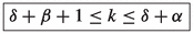
Consider two elements, $\alpha$ and $\delta$, such that $\alpha >0$, $1\le \delta <n$, and that satisfy the following conditions:

$$\begin{aligned} \begin{array}{ll} a_{\sigma (\delta +1)}{{\mathcal {R}}}a_{\sigma (\delta +\alpha )}&{}\\ a_{\sigma (i)}\lnot {{\mathcal {R}}} a_{\sigma (j)} &{}\text {if }i\le \delta , \; \forall \, j\in \{i+1,\ldots ,n\} , \\ a_{\sigma (\delta +1)}\lnot {{\mathcal {R}}} a_{\sigma (i)}&{}\forall \, i\in \{\delta +\alpha +1,\ldots ,n\}. \end{array} \end{aligned}$$

We select the indices $J=\{j_1, \ldots , j_\beta \}$ with $1<j_1< \cdots < j_\beta =\alpha$ such that $\forall \delta +\alpha <k\le n$, $a_{\sigma (\delta +j_k)}\lnot {{\mathcal {R}}} a_{\sigma (\delta +1)}$ and consider

$$\begin{aligned} I=\{1,2,\ldots ,\alpha \}-J=\{i_1,i_2, \ldots ,i_{\alpha -\beta }\} \end{aligned}$$

with $1=i_1<i_2< \cdots<i_{\alpha -\beta }<\alpha$ (it’s clear that $a_{\sigma (\delta +i_k)}{{\mathcal {R}}}a_{\sigma (\delta +1)}$ and $a_{\sigma (\delta +1)}\lnot {{\mathcal {R}}} a_{\sigma (\delta +i_k)}$).

In these conditions, the permutation

$$\begin{aligned} \sigma _{\delta \alpha }= & {} \big ( {\sigma (1)},\ldots ,{\sigma (\delta )}, {\sigma (\delta +j_1)},\ldots ,{\sigma (\delta +j_\beta )},\\{} & {} {\sigma (\delta +i_1)},\ldots ,{\sigma (\delta +i_{\alpha -\beta })}, {\sigma (\delta +\alpha +1)}, \ldots ,{\sigma (n)}\big ) \end{aligned}$$

is called the basic permutation of $\sigma$ for ${{\mathcal {R}}}$.

Remark 4.2

The previous definition can be interpreted in terms of the adjacency matrix associated with the initial permutation $\sigma$ as follows.

Let be $(S,{{\mathcal {R}}})$ a poset and $M^\sigma \in {{\mathcal {M}}}_S({{\mathcal {R}}})$ with $\sigma$ a non compatible permutation, that is, $M^\sigma$ is not lower triangular.

We consider two elements $\alpha$ and $\delta$ such that $\alpha >0$, $1< \delta <n$, and

$$\begin{aligned} \begin{array}{ll} m_{\delta +1, \delta +\alpha }=1 &{} \\ m_{i,j}=0 &{}\text {if }i\le \delta , \; \forall \, j\in \{i+1,\ldots ,n\} ,\; \\ m_{\delta +1, i}=0 &{} \forall \, i\in \{\delta +\alpha +1,\ldots ,n\}. \end{array} \end{aligned}$$

We select the indices $J=\{j_1, \ldots , j_\beta \}$ with $1<j_1< \cdots < j_\beta =\alpha$ such that $\forall \delta +\alpha <k\le n$, $m_{\delta +j_k, \delta +1}=0$ and consider

$$\begin{aligned} I=\{1,2,\ldots ,\alpha \}-J=\{i_1,i_2, \ldots ,i_{\alpha -\beta }\} \end{aligned}$$

with $1=i_1<i_2< \cdots<i_{\alpha -\beta }<\alpha$ (it’s clear that $m_{\delta +i_k,\delta +1}=1$ and $m_{\delta +1,\delta +i_k}=0$).

Example 4.2

Continuing with the same ordered set of Example 3.5 and taking as initial permutation

$$\begin{aligned} \sigma =(2,1,3,6,7,4,5,8,9) \end{aligned}$$

which, as can be easily checked, is not compatible with the relation ${{{\mathcal {R}}}}$ (for example it can be seen that $a_9\lnot {{\mathcal {R}}} a_7$ and yet, $a_9{{\mathcal {T}}}_\sigma a_7$ with the order relation induced by the order of the permutation).

The adjacency matrix for $\sigma$ is:

$$\begin{aligned} M^\sigma ={ \left( \begin{array}{ccccccccc} 1 &{} \quad 0 &{} \quad 0 &{} \quad 0 &{} \quad 0 &{} \quad 0 &{} \quad 0 &{} \quad 0 &{} \quad 0\\ 0 &{} \quad 1 &{} \quad 0 &{} \quad 0 &{} \quad 0 &{} \quad 0 &{} \quad 0 &{} \quad 0 &{} \quad 0\\ 1 &{} \quad 1 &{} \quad 1 &{} \quad 0 &{} \quad 0 &{} \quad 0 &{} \quad 0 &{} \quad 0 &{} \quad 0\\ 0 &{} \quad 0 &{} \quad 0 &{} \quad 1 &{} \quad 0 &{} \quad 0 &{} \quad 1 &{} \quad 0 &{} \quad 0\\ 1 &{} \quad 1 &{} \quad 1 &{} \quad 0 &{} \quad 1 &{} \quad 1 &{} \quad 1 &{} \quad 0 &{} \quad 0\\ 1 &{} \quad 1 &{} \quad 1 &{} \quad 0 &{} \quad 0 &{} \quad 1 &{} \quad 0 &{} \quad 0 &{} \quad 0\\ 0 &{} \quad 0 &{} \quad 0 &{} \quad 0 &{} \quad 0 &{} \quad 0 &{} \quad 1 &{} \quad 0 &{} \quad 0\\ 1 &{} \quad 1 &{} \quad 1 &{} \quad 0 &{} \quad 0 &{} \quad 1 &{} \quad 0 &{} \quad 1 &{} \quad 0\\ 1 &{} \quad 1 &{} \quad 1 &{} \quad 0 &{} \quad 1 &{} \quad 1 &{} \quad 1 &{} \quad 1 &{} \quad 1 \end{array}\right) .} \end{aligned}$$

If we apply the basic permutation to $\sigma$ we obtain the new permutation

$$\begin{aligned} \sigma _{\delta \alpha }=(2,1,3,7,4,5,6,8,9) \end{aligned}$$

because, taking $\delta =3$ and $\alpha =4$, the conditions of the Definition 4.1 are verified.

Next, we prove that, after performing each basic permutation on a permutation, we are getting totally compatible elements.

Theorem 4.2

Let (S, R) be a poset, $\sigma =({\sigma (1)},{\sigma (2)}, \ldots , {\sigma (n)})$ a permutation of elements of S and $\sigma _{\delta \alpha }$ the basic permutation of $\sigma$ for ${{\mathcal {R}}}$, then, with the notation of the Definition 4.1, $a_{\sigma (\delta +1)}$ is totally compatible for the permutation $\sigma _{\delta \alpha }$.

Proof

Firstly, if $\sigma _{\delta \alpha }$ is the basic permutation for $\sigma$, we note ${\sigma (\delta +1)}=\sigma _{\delta \alpha }(\delta +\beta +1)$

We are going to separate 4 cases:

• 1. $\Rightarrow$ $a_{\sigma _{\delta \alpha }(k)}=a_{\sigma (k)}$ and $a_{\sigma (k)}\lnot {{\mathcal {R}}} a_{\sigma (\delta +1)}$ but $a_{\sigma (\delta +1)}=a_{\sigma _{\delta \alpha }(\delta +\beta +1)}$ because $k\le \delta$, so $a_{\sigma _{\delta \alpha }(k)}\lnot {{\mathcal {R}}} a_{\sigma _{\delta \alpha }(\delta +\beta +1)}$.

• 2. $\Rightarrow$ ($k=k'+\delta \rightarrow 1\le k'\le \beta$) $\Rightarrow$ $a_{\sigma _{\delta \alpha }(k)}=a_{\sigma _{\delta \alpha }(\delta +k')}=a_{\sigma (\delta +j_{k'})}\text { and }a_{\sigma (\delta +j_{k'})} \lnot {{\mathcal {R}}} a_{\sigma ( \delta +1)}$ but $a_{\sigma ( \delta +1)}=a_{\sigma _{\delta \alpha }(\delta +\beta +1)}$, so $a_{\sigma _{\delta \alpha }(k)}\lnot {{\mathcal {R}}} a_{\sigma _{\delta \alpha }(\delta +\beta +1)}$.

• 3. $\Rightarrow$ ($k=k'+\delta +\beta \rightarrow 1\le k'\le \alpha -\beta$) $\Rightarrow$ $a_{\sigma _{\delta \alpha }({\delta +\beta +1})}=a_{\sigma ( \delta +1)}\text { and }a_{\sigma ( \delta +1)}\lnot {{\mathcal {R}}} a_{\sigma (\delta +i_{k'})}$ but $a_{\sigma (\delta +i_{k'})}=a_{\sigma _{\delta \alpha }({ \delta +\beta +k'})}=a_{\sigma _{\delta \alpha }({k})}$, so $a_{\sigma _{\delta \alpha }({\delta +\beta +1})}\lnot {{\mathcal {R}}} a_{\sigma _{\delta \alpha }({k})}$.

• 4. $\Rightarrow$ $a_{\sigma _{\delta \alpha }({\delta +\beta +1})}=a_{\sigma ( \delta +1)}\text { and }a_{\sigma ( \delta +1)}\lnot {{\mathcal {R}}} a_{\sigma ( k)}\text { but }a_{\sigma ( k)}=a_{\sigma _{\delta \alpha }({k})}$, so $a_{\sigma _{\delta \alpha }({\delta +\beta +1})}\lnot {{\mathcal {R}}} a_{\sigma _{\delta \alpha }({k})}$.

Therefore, $\forall \,j,\,k$ such that $1\le j<\delta +\beta +1<k\le n$, $a_{\sigma _{\delta \alpha }({j})}\lnot {{\mathcal {R}}} a_{\sigma _{\delta \alpha }({{\delta +\beta +1}})}$ and $a_{\sigma _{\delta \alpha }({\delta +\beta +1})}\lnot {{\mathcal {R}}} a_{\sigma _{\delta \alpha }({k})}$ then $a_{\sigma ( \delta +1)}=a_{\sigma _{\delta \alpha }({\delta +\beta +1})}$ is totally compatible for the permutation $\sigma _{\delta \alpha }$. $\square$

Remark 4.3

As already mentioned in the Remark 3.2 regarding the totally compatible elements, since $b_{\delta +\beta +1}$ is totally compatible for $\sigma _{\delta \alpha }$, if $M^{\sigma _{\delta \alpha }}$ is the adjacency matrix associated to the permutation $\sigma _{\delta \alpha }$ then

$$\begin{aligned} \begin{array}{ll} m_{i,\delta +\beta +1}=0&{}\quad \forall i<\delta +\beta +1 \text{ and } \\ m_{\delta +\beta +1,j}=0&{}\quad \forall \delta +\beta +1<j. \end{array} \end{aligned}$$

The following result proves that with the performance of each basic permutation the condition of total compatibility is not lost, i.e., that the totally compatible elements in the initial permutation remain totally compatible in the final permutation.

Theorem 4.3

Let (S, R) be a poset, $a_{\sigma (i_0)}$ totally compatible for a permutation $\sigma$ and $\sigma _{\delta \alpha }$ the basic permutation of $\sigma$ for ${{\mathcal {R}}}$ then $a_{\sigma (i_0)}$ is totally compatible for the permutation $\sigma _{\delta \alpha }$.

Proof

If $\sigma _{\delta \alpha }$ is the basic permutation for $\sigma$, we observe $\sigma (i_0)\not =\delta +1$ and $\sigma (i_0)\not =\delta +\alpha$.

Depending on the position of the element $a_{\sigma (i_0)}$ in the permutation, we will distinguish three cases:

• 1. $\Rightarrow {\sigma _{\delta \alpha }(i_0)}={\sigma (i_0)}$

  • if $j<\sigma (i_0)$ then $a_{\sigma _{\delta \alpha }(j)}=a_{\sigma (j)}$, so $a_{\sigma _{\delta \alpha }(j)}\lnot {{\mathcal {R}}} a_{\sigma (i_0)}$

  • if $\sigma (i_0)<k$ then $\sigma (i_0)<\sigma (k)\Rightarrow a_{\sigma (i_0)}\lnot {{\mathcal {R}}} a_{\sigma (k)}=a_{\sigma _{\delta \alpha }(k)}.$

• 2.

  By the transitivity of the relation, we know that $a_{\sigma (i_0)}\lnot {{\mathcal {R}}} a_{\sigma (\delta +1)}$, since otherwise we would reach a contradiction because, as $a_{\sigma (\delta +1)}{{\mathcal {R}}}a_{\sigma (\delta +\alpha )}$, we would have that $a_{\sigma (i_0)}{{\mathcal {R}}}a_{\sigma (\delta +\alpha )}$, but $a_{\sigma (i_0)}$ is totally compatible.

  Using the notation of the Definition 4.1$\sigma (i_0)\in J \,\Rightarrow \, \sigma (i_0)=j_{r_0}=\delta +r_0$.

  Let $t\le \sigma (i_0)= \delta +r_0$.

  We will distinguish 5 cases.

  • (a) then $t=\sigma (t)$ and $a_{\sigma _{\delta \alpha }(t)}=a_{\sigma (t)}\lnot {{\mathcal {R}}} a_{\sigma (i_0)}$

  • (b) then $t=j_{r_0-\delta }<j_{r_0}=\sigma (i_0)\Rightarrow$

    $$\begin{aligned} a_{\sigma _{\delta \alpha }(t)}=a_{\sigma (j_{r_0}-\delta )}\lnot {{\mathcal {R}}} a_{\sigma (j_{r_0})}=a_{\sigma (i_0)} \end{aligned}$$

    since $a_{\sigma (i_0)}$ is totally compatible for $\sigma$.

  • (c) then $\sigma (i_0)=j_{r_0}=\delta +r_0< t=\delta +r_0+\omega =j_{r_0+\omega } \text{ with } 1\le \omega \le \beta -r_0 \Rightarrow$

    $$\begin{aligned} a_{\sigma (i_0)}\lnot {{\mathcal {R}}} a_{\sigma (j_{r_0+\omega })}=a_{\sigma (t)}=a_{\sigma _{\delta \alpha }(t)} \end{aligned}$$

    because $a_{\sigma (i_0)}$ is totally compatible for $\sigma$.

  • (d) then $t\in I$ and $a_{\sigma _{\delta \alpha }(t)}=a_{\sigma (\delta +i_\omega )}$ with $1\le \omega \le \alpha -\beta$ and $a_{\sigma (i_0)}\lnot {{\mathcal {R}}} a_{\sigma _{\delta \alpha }(t)}$ because, otherwise, as we have seen above, we would reach a contradiction since, due to the transitivity of the relation, we get

    $$\begin{aligned} a_{\sigma (i_0)}{{\mathcal {R}}}a_{\sigma (\delta +i_\omega )}{{\mathcal {R}}}a_{\sigma (\delta +1)}. \end{aligned}$$
  • (e)

    Similar to case (2a) since $\sigma (t)=t$ and, therefore $a_{\sigma (t)}=a_{\sigma _{\delta \alpha }(t)}$.

• 3. Similar to case (2a) because also $a_{\sigma _{\delta \alpha }(i_0)}=a_{\sigma (i_0)}$

  • if $j<\sigma (i_0)$ then $\sigma (j)<\sigma (i_0)\Rightarrow a_{\sigma _{\delta \alpha }(j)}=a_{\sigma (j)}\lnot {{\mathcal {R}}} a_{\sigma (i_0)}$

  • if $\sigma (i_0)<k$ then $a_{\sigma (i_0)}\lnot {{\mathcal {R}}} a_{\sigma (k)}=a_{\sigma _{\delta \alpha }(k)}$

So $a_{\sigma (i_0)}$ is totally compatible for the permutation $\sigma _{\delta \alpha }$. $\square$

Remark 4.4

If $M^{\sigma }$ is the adjacency matrix associated to $\sigma$ and $M^{\sigma _{\delta \alpha }}$ is the adjacency matrix associated to $\sigma _{\delta \alpha }$ then

$$\begin{aligned} \begin{array}{ll} m_{i,\delta +\beta +1}=0 &{}\quad \forall i<\delta +\beta +1\,\, \text{ and } \\ m_{\delta +\beta +1,j}=0&{}\quad \forall \delta +\beta +1<j. \end{array} \end{aligned}$$

Corollary 4.2

After at most $n-1$ repetitions of the basic permutation over an initial permutation, a permutation compatible with the order relation is obtained.

In this example, we need to perform the basic permutation process $n-1$ times to obtain a compatible permutation.

Example 4.3

Initially, we consider $\gamma =(n,\ldots ,1)$, and we need to perform the basic permutation process $n-1$ times to obtain $\sigma =( 1,\ldots , n)$ which is the only permutation in which all elements are totally compatible with the relation ${{\mathcal {T}}}_\sigma$.

Remark 4.5

When applying genetic algorithms, the search for random compatible orders plays a crucial role. These outcomes allow us, given any random order, to generate a compatible order in at most $n-1$ iterations, where n is the number of elements in the set.

Example 4.4

Continuing with the Example 4.2 where

$$\begin{aligned} \sigma =( 2, 1, 3, 6, 7, 4, 5, 8, 9). \end{aligned}$$

Applying the basic permutation to $\sigma$ we obtained

$$\begin{aligned} \sigma _{34}=( 2, 1, 3, 7, 4, 5, 6, 8, 9) \end{aligned}$$

in which we can observe that, as stated in Theorem 4.2, $a_6$ is totally compatible and, as stated in Theorem 4.3, $a_2, a_1, a_3, a_8$ and $a_9$ are still totally compatible as they were in $\sigma$.

Its adjacency matrix is:

$$\begin{aligned} M^{\sigma _{34}}={\left( \begin{array}{ccccccccc} 1 &{} \quad 0 &{} \quad 0 &{} \quad 0 &{} \quad 0 &{} \quad 0 &{} \quad 0 &{} \quad 0 &{} \quad 0\\ 0 &{} \quad 1 &{} \quad 0 &{} \quad 0 &{} \quad 0 &{} \quad 0 &{} \quad 0 &{} \quad 0 &{} \quad 0\\ 1 &{} \quad 1 &{} \quad 1 &{} \quad 0 &{} \quad 0 &{} \quad 0 &{} \quad 0 &{} \quad 0 &{} \quad 0\\ 1 &{} \quad 1 &{} \quad 1 &{} \quad 1 &{} \quad 1 &{} \quad 1 &{} \quad 0 &{} \quad 0 &{} \quad 0\\ 1 &{} \quad 1 &{} \quad 1 &{} \quad 0 &{} \quad 1 &{} \quad 0 &{} \quad 0 &{} \quad 0 &{} \quad 0\\ 0 &{} \quad 0 &{} \quad 0 &{} \quad 0 &{} \quad 0 &{} \quad 1 &{} \quad 0 &{} \quad 0 &{} \quad 0\\ 0 &{} \quad 0 &{} \quad 0 &{} \quad 0 &{} \quad 0 &{} \quad 1 &{} \quad 1 &{} \quad 0 &{} \quad 0\\ 1 &{} \quad 1 &{} \quad 1 &{} \quad 0 &{} \quad 1 &{} \quad 0 &{} \quad 0 &{} \quad 1 &{} \quad 0\\ 1 &{} \quad 1 &{} \quad 1 &{} \quad 1 &{} \quad 1 &{} \quad 1 &{} \quad 0 &{} \quad 1 &{} \quad 1 \end{array}\right) .} \end{aligned}$$

After performing all the possible basic permutations, we obtain the permutation

$$\begin{aligned} \gamma =( 2, 1, 3, 4, 5, 7, 6, 8, 9) \end{aligned}$$

that we can see that all its elements are totally compatible, and whose adjacency matrix is:

$$\begin{aligned} M^\gamma ={ \left( \begin{array}{ccccccccc} 1 &{} \quad 0 &{} \quad 0 &{} \quad 0 &{} \quad 0 &{} \quad 0 &{} \quad 0 &{} \quad 0 &{} \quad 0\\ 0 &{} \quad 1 &{} \quad 0 &{} \quad 0 &{} \quad 0 &{} \quad 0 &{} \quad 0 &{} \quad 0 &{} \quad 0\\ 1 &{} \quad 1 &{} \quad 1 &{} \quad 0 &{} \quad 0 &{} \quad 0 &{} \quad 0 &{} \quad 0 &{} \quad 0\\ 1 &{} \quad 1 &{} \quad 1 &{} \quad 1 &{} \quad 0 &{} \quad 0 &{} \quad 0 &{} \quad 0 &{} \quad 0\\ 0 &{} \quad 0 &{} \quad 0 &{} \quad 0 &{} \quad 1 &{} \quad 0 &{} \quad 0 &{} \quad 0 &{} \quad 0\\ 1 &{} \quad 1 &{} \quad 1 &{} \quad 1 &{} \quad 1 &{} \quad 1 &{} \quad 0 &{} \quad 0 &{} \quad 0\\ 0 &{} \quad 0 &{} \quad 0 &{} \quad 0 &{} \quad 1 &{} \quad 0 &{} \quad 1 &{} \quad 0 &{} \quad 0\\ 1 &{} \quad 1 &{} \quad 1 &{} \quad 1 &{} \quad 0 &{} \quad 0 &{} \quad 0 &{} \quad 1 &{} \quad 0\\ 1 &{} \quad 1 &{} \quad 1 &{} \quad 1 &{} \quad 1 &{} \quad 1 &{} \quad 0 &{} \quad 1 &{} \quad 1 \end{array}\right) .} \end{aligned}$$

5 Conclusions and Future Research

As mentioned in the introduction, this work arises from a collaborative project with the industry, with the objective to optimize the additive manufacturing (AM) process, which involves printing three-dimensional objects in overlapping layers.

In this process, there is a factor that determines the order in which the printing of each layer must follow.

This factor defines the process model proposed in this work, as it establishes an order relation that must be respected for the correct printing of the objects.

In this work, results are presented that ensure the existence of such orders and procedures to construct them. They are also characterized by both their associated adjacency matrices and the compatibility of their elements.

Furthermore, an algorithm is provided that, starting from a random permutation, finds the closest compatible permutation in the sense that it minimizes the number of steps to achieve it.

In order to achieve our objective of optimizing the AM process, several lines of future action have been considered, including: determining the optimal compatible permutation in the sense of minimizing the printing cost of each layer; attempting to bound or determine the number of compatible permutations for each layer; investigating the conditions under which a compatible order for one layer can be applied to the next layer, considering that successive printing layers may have a similar arrangement of objects; and lastly, taking into account that the solution space can be on the order of 3000!, finding strategies to simplify the solution space, i.e., organizing the information to reduce the solution space.

References

Birkhoff, G.: Lattice Theory. American Mathematical Society, Providence (1948)
Caspard, N., Leclerc, B., Monjardet, B.: Finite Ordered Sets. Concepts, Results and Uses. Encyclopedia of Mathematics and Its Applications, 144. Cambridge University Press, Cambridge (2012)
Chowdhury, S., Yadaiah, N., Prakash, C., Ramakrishna, S., Dixit, S., Gupta, L.R., Buddhi, D.: Laser powder bed fusion: a state-of-the-art review of the technology, materials, properties & defects, and numerical modelling. J. Market. Res. 20, 2109–2172 (2022). https://doi.org/10.1016/j.jmrt.2022.07.121
Garg, V.K.: Introduction to Lattice Theory with Computer Science Applications. Wiley, Hoboken (2015)
Khorasani, A., Gibson, I., Veetil, J.K., et al.: A review of technological improvements in laser-based powder bed fusion of metal printers. Int. J. Adv. Manuf. Technol. 108, 191–209 (2020). https://doi.org/10.1007/s00170-020-05361-3
Olleak, A., Xi, Z.: Efficient LPBF process simulation using finite element modeling with adaptive remeshing for distortions and residual stresses prediction. Manuf. Lett. 24, 140–144 (2020). https://doi.org/10.1016/j.mfglet.2020.05.002. (ISSN 2213-8463)
Viguerie, A., Bertoluzzo, S., Auricchio, F.: A fat boundary-type method for localized nonhomogeneous material problems. Comput. Methods Appl. Mech. Eng. (2020). https://doi.org/10.1016/j.cma.2020.112983
Acknowledgements
This work has been partially supported by the collaborative project FUO-115-22.
Funding
Open Access funding provided thanks to the CRUE-CSIC agreement with Springer Nature.
Author information
Authors and Affiliations
Corresponding author
Additional information
Communicated by Zenon Mróz.
Publisher's Note
Springer Nature remains neutral with regard to jurisdictional claims in published maps and institutional affiliations.
Rights and permissions
Open Access This article is licensed under a Creative Commons Attribution 4.0 International License, which permits use, sharing, adaptation, distribution and reproduction in any medium or format, as long as you give appropriate credit to the original author(s) and the source, provide a link to the Creative Commons licence, and indicate if changes were made. The images or other third party material in this article are included in the article’s Creative Commons licence, unless indicated otherwise in a credit line to the material. If material is not included in the article’s Creative Commons licence and your intended use is not permitted by statutory regulation or exceeds the permitted use, you will need to obtain permission directly from the copyright holder. To view a copy of this licence, visit http://creativecommons.org/licenses/by/4.0/.
About this article
Cite this article
Abascal, P., Fueyo, F., Jiménez, J. et al. Compatible TOSets with POSets: An Application to Additive Manufacturing. J Optim Theory Appl 201, 177–198 (2024). https://doi.org/10.1007/s10957-024-02388-4
Received:
Accepted:
Published:
Issue Date:
DOI: https://doi.org/10.1007/s10957-024-02388-4