
Abstract
In this paper, we use techniques of Malliavin calculus and forward integration to present a general stochastic maximum principle for anticipating stochastic differential equations driven by a Lévy type of noise. We apply our result to study a general stochastic differential game problem of an insider.
References
An, T., Øksendal, B., Okur, Y.: A Malliavin calculus approach to general stochastic differential games with partial information. In: Malliavin Calculus and Stochastic Analysis. Springer Proceedings in Mathematics & Statistics, vol. 34, pp. 489–510. Springer, Berlin (2013)
Di Nunno, G., Menoukeu-Pamen, O., Øksendal, B., Proske, F.: A general maximum principle for anticipative stochastic control and applications to insider trading. In: Advanced Mathematical Methods for Finance, pp. 181–221. Springer, Berlin (2011)
Ewald, C.O., Xiao, Y.: Information: price and impact on general welfare and optimal investment. An anticipating stochastic differential game model. Adv. in Appl. Probab. 43(1), 97–120 (2011)
Øksendal, B., Zhang, T.: The Itô-Ventzell formula and forward stochastic differential equations driven by Poisson random measures. Osaka Journal of Mathematics 44(1), 207–230 (2007)
Russo, F., Vallois, P.: Forward, backward and symmetric stochastic integration. Probability Theory and Related Fields 97, 403–421 (1993)
Di Nunno, G., Meyer-Brandis, T., Øksendal, B., Proske, F.: Malliavin calculus and anticipative Itô formulae for Lévy processes. Inf. Dim. Anal. Quant. Probab. 8, 235–258 (2005)
Ghomrasni, R., Menoukeu-Pamen, O.: An approximation of the generalized covariation process In: Anticipative Stochastic Calculus with Applications to Financial Markets. PhD thesis, pp. 17–44, University of the Witwatersrand (2009)
Nualart, D., Pardoux, E.: Stochastic calculus with anticipating integrands. Probability Theory and Related Fields 78, 535–581 (1988)
Russo, F., Vallois, P.: Stochastic calculus with respect to continuous finite variation processes. Stochastics and Stochastics Reports 70, 1–40 (2000)
Di Nunno, G., Øksendal, B., Proske, F.: Malliavin Calculus for Lévy Processes with Applications to Finance. Universitext. Springer, Birlin (2008)
Nualart, D.: The Malliavin Calculus and Related Topics. Springer, Berlin (1995)
Bertoin, J.: Lévy Processes. Cambridge Tracts in Mathematics, vol. 121. Cambridge University Press, Cambridge (1996)
Sato, K.I.: Lévy Processes and Infinitely Divisible Distributions. Cambridge Studies in Advanced Mathematics, vol. 68. Cambridge University Press, Cambridge (1999)
Itô, K.: Generalized Poisson functionals. Probability Theory Related Fields 77, 1–28 (1988)
Kohatsu-Higa, A., Sulem, A.: Utility maximization in an insider influenced market. Mathematical Finance 16(1), 153–179 (2006)
Baghery, F., Øksendal, B.: A maximum principle for stochastic control with partial information. Stochastic Analysis and Applications 25, 705–717 (2007)
Nualart, D., Üstünel, A., Zakai, E.: Some relations among classes of σ-fields on wiener space. Probability Theory and Related Fields 85, 119–129 (1990)
Menoukeu-Pamen, O., Meyer-Brandis, T., Nilssen, T., Proske, F., Zhang, T.: A variational approach to the construction and Malliavin differentiability of strong solutions of SDEs. Math. Ann. (2013). doi:10.1007/s00208-013-0916-3
Acknowledgements
The authors are grateful to two anonymous referees and Professor Franco Giannessi for their helpful comments and suggestions.
The research leading to these results has received funding from the European Research Council under the European Community’s Seventh Framework Programme (FP7/2007-2013) /ERC grant agreement No. [228087].
Author information
Authors and Affiliations
Corresponding author
Additional information
Communicated by Negash G. Medhin.
Appendix: Proof of Theorem 4.1
Appendix: Proof of Theorem 4.1
Proof
The proof relies on a combination of arguments of Refs. [1] and [2].
-
(i)
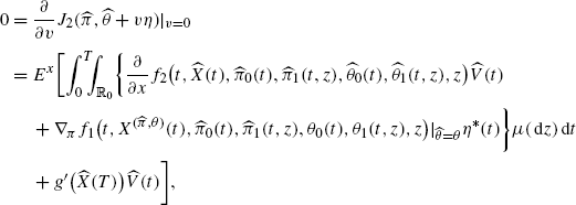
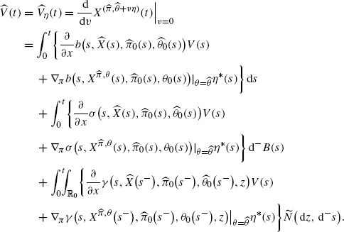
Suppose \((\widehat{\pi},\widehat{\theta})\in\mathcal{A}_{\varPi}\times \mathcal{A}_{\varTheta}\) is a Nash-equilibrium. Since 1 and 2 hold for all π and \(\theta, (\widehat{\pi}, \widehat{\theta})\) is a directional critical point for J i (π,θ) for i=1,2 in the sense that, for all bounded \(\beta\in\mathcal{A}_{\varPi}\) and \(\eta\in \mathcal{A}_{\varTheta}\), there exists δ>0 such that \(\widehat{\pi }+y\beta\in\mathcal{A}_{\varPi}, \widehat{\theta}+v\eta\in\mathcal {A}_{\varTheta}\) for all y,v∈]−δ,δ[. Then we have
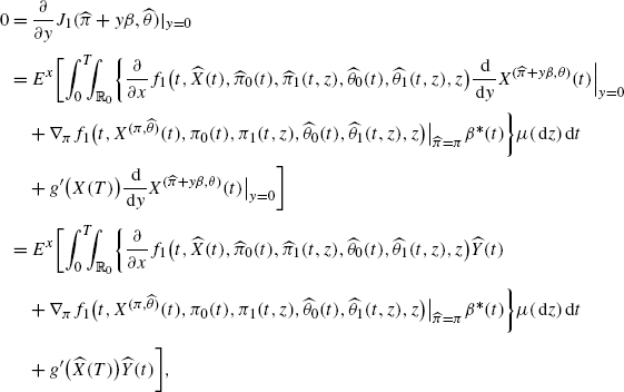 (A.1)
(A.1)where
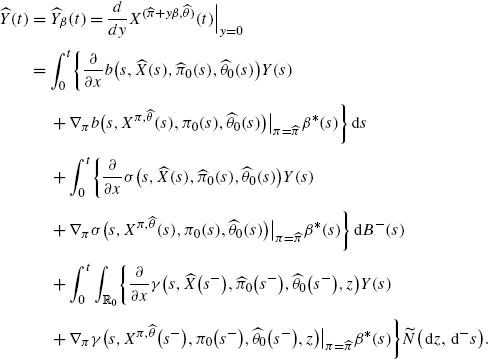 (A.2)
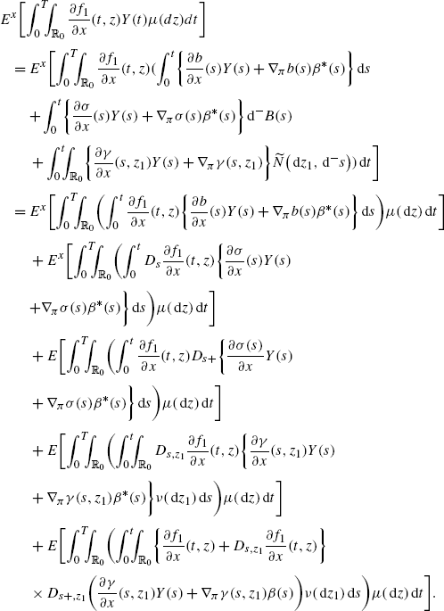
(A.2)We study the three summands separately. Using the short notation
$$\frac{\partial}{\partial x }f_1\bigl(t,\widehat{X}(t),\widehat{\pi },\widehat{\theta},z\bigr)=\frac{\partial}{\partial x }f_1(t,z),\quad \nabla_\pi f_1 \bigl(t,X^{(\pi,\widehat{\theta})}(t),\pi,\widehat{\theta },z\bigr)\big \vert _{\widehat{\pi}=\pi}$$and similarly for \(\frac{\partial}{\partial x }b, \nabla_{\pi}b, \frac{\partial}{\partial x }\sigma, \nabla_{\pi}\sigma, \frac {\partial}{\partial x }\gamma\) and ∇ π γ. By the duality formulas (20) and (23) and the Fubini theorem, we get
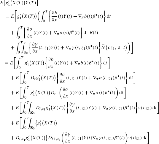
Changing notation z 1→z, this becomes
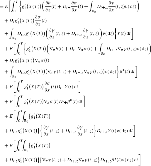 (A.3)
(A.3)Here, we used the multidimensional product rule for Malliavin derivatives. Similarly, by using both Fubini and duality formulas (20) and (23), we get
Changing notation t 1→t and z 1→z, this becomes
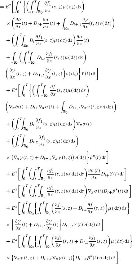 (A.4)
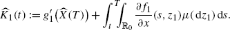
(A.4)Recall that
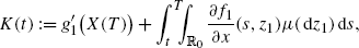
so
 (A.5)
(A.5)By combining (A.3)–(A.4), we get
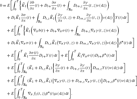 (A.6)
(A.6)Now, apply this to \(\beta=\beta_{\alpha}\in\mathcal{A}_{\varPi}\) given as β α (s):=αχ [t,t+h](s), for some t,h∈]0,T[, t+h≤T, where, α=α(ω) is bounded and \(\mathcal{G}^{2}_{t}\)-measurable. Then \(Y^{(\beta_{\alpha})}(s)=0\) for 0≤s≤t and (A.6) becomes
 (A.7)
(A.7)where

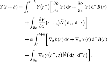
Note that, by the definition of Y, with \(Y(s)=Y^{(\beta_{\alpha })}(s)\) and s≥t+h, the process Y(s) follows the dynamics
 (A.8)
(A.8)for s≥t+h with initial condition Y(t+h) in time t+h. By the Itô formula for forward integrals, this equation can be solved explicitly, and we get
 (A.9)
(A.9)where, in general, for s≥t,
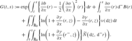
Note that G(t,s) does not depend on h, but Y(s) does. Defining \(H^{1}_{0}\) as in (30), it follows that
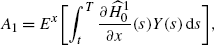
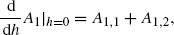
where \(\widehat{H}^{1}_{0}(s)=H^{1}_{0}(s,\widehat{X}(s),\widehat{\pi},\widehat {\theta} )\). Differentiating with respect to h at h=0, we get

Since Y(t)=0, we see that
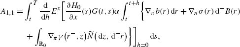
$$\frac{ \,\mathrm {d}}{ \,\mathrm {d}h }E^x \biggl[\int_t^{t+h} \frac{\partial H_0}{\partial x }(s)Y(s)\,\mathrm {d}s \biggr]_{h=0}=0. $$Therefore, by (A.9),
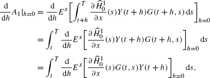
where Y(t+h) is given by
Therefore, by the two preceding equalities,
where
and
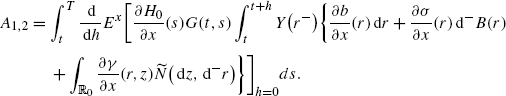
Applying once more the duality formula, we have
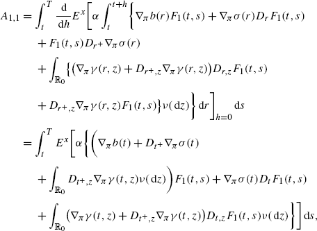
where we have
$$F_1(t,s)=\frac{\partial\widehat{H}^1_0}{\partial x }(s)G(t,s). $$Since Y(t)=0, we see that A 1,2=0. We conclude that
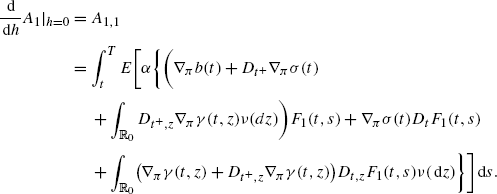 (A.10)
Moreover,
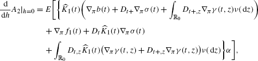 (A.11)
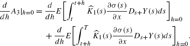
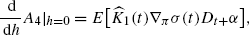 (A.12)
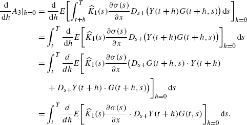
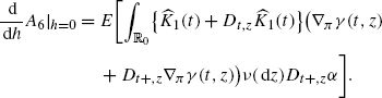 (A.13)
On the other hand, differentiating A 3 with respect to h at h=0, we get
Since Y(t)=0, we get
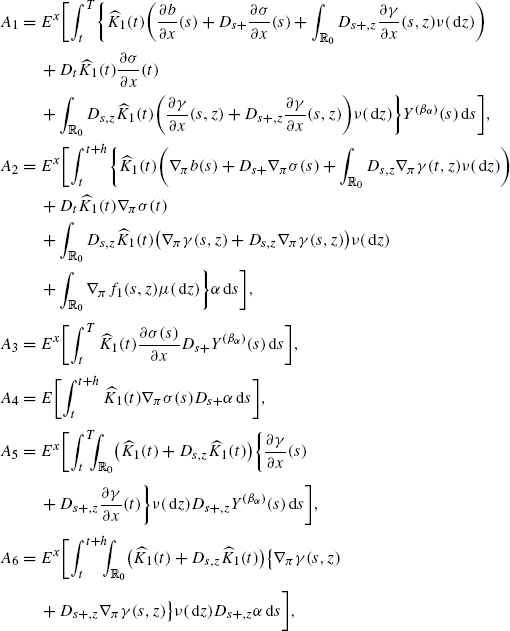
Using the definition of \(\widehat{p}\) and \(\widehat{H}_{1}\) given respectively by (39) and (38) in the theorem, it follows from (A.7) that
$$ E \bigl[ \nabla_\pi\widehat{H}_1\bigl(t, \widehat{X }(t),\widehat {u}(t)\bigr)\vert \mathcal{G}^2_{t} \bigr] + E[A]=0\quad\text{a.e. in\ }(t,\omega), $$(A.14)where
 (A.15)
Similarly, we have
 (A.16)
where
 (A.17)
Define
$$D(s)=D(t+h)G(t+h,s);\quad s \geq t+h, $$where G(t,s) is defined as in (42). Using similar arguments, we get
$$E \bigl[ \nabla_\pi\widehat{H}_2\bigl(t, \widehat{X }(t),\widehat {u}(t)\bigr)\vert \mathcal{G}^1_{t} \bigr] + E[B]=0\quad\text{a.e. in \ }(t,\omega), $$where B is given in the same way as A. This completes the proof of (i).
-
(ii)
Conversely, suppose that there exists \(\widehat{\pi}\in\mathcal{A}_{\varPi}\) such that (36) holds. Then, by reversing the previous arguments, we obtain that (A.7) holds for all \(\beta_{\alpha}(s):=\alpha\chi_{[ t,t+h]}(s) \in\mathcal {A}_{\varPi}\), where
for some t,h∈]0,T[,t+h≤T, where α=α(ω) is bounded and \(\mathcal{G}^{2}_{t}\)-measurable. Hence, these equalities hold for all linear combinations of β α . Since all bounded \(\beta\in\mathcal{A}_{\varPi}\) can be approximated pointwise boundedly in (t,ω) by such linear combinations, it follows that (A.7) holds for all bounded \(\beta\in\mathcal{A}_{\varPi}\). Hence, by reversing the remaining part of the previous proof, we conclude that
$$\frac{\partial J_1}{\partial y}(\widehat{\pi}+y\beta, \widehat {\theta})\vert _{y=0}=0,\quad\text{for all } \beta. $$Similarly, suppose that there exists \(\widehat{\theta}\in\mathcal {A}_{\varTheta}\) such that 37 holds. Then, the above argument leads us to conclude that
$$\frac{\partial J_2}{\partial v}(\widehat{\pi}, \widehat{\theta }+v\eta)\vert _{v=0}=0,\quad\text{for all } \eta. $$On the other hand, assume moreover that \(\pi\rightarrow J_{1}(\pi, \widehat{\theta})\), then
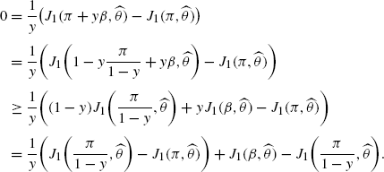
Taking the limit for y→0 and using the fact that \({\lim}_{y\rightarrow0}\frac{1}{y} (J_{1}(\frac{\pi}{1-y},\widehat {\theta})-J_{1}(\pi, \widehat{\theta}) )=0\), we obtain that \(0\geq J_{1}(\beta, \widehat{\theta})-J_{1}(\widehat{\pi},\widehat{\theta})\). Since β can be chosen within the set \(\mathcal{A}_{\pi}\), we obtain by formally setting β=π that
 (A.18)
Analogously, we obtain
 (A.19)
This means that \((\widehat{\pi},\widehat{\theta})\) is a Nash-equilibrium for the market. is concave in each π or θ.
This completes the proof.


□
Rights and permissions
About this article
Cite this article
Pamen, O.M., Proske, F. & Salleh, H.B. Stochastic Differential Games in Insider Markets via Malliavin Calculus. J Optim Theory Appl 160, 302–343 (2014). https://doi.org/10.1007/s10957-013-0310-z
Received:
Accepted:
Published:
Issue Date:
DOI: https://doi.org/10.1007/s10957-013-0310-z