An Adaptive Orthogonal Basis Method for Computing Multiple Solutions of Differential Equations with Polynomial Nonlinearities

Abstract

This paper presents an innovative approach, the Adaptive Orthogonal Basis Method, tailored for computing multiple solutions to differential equations characterized by polynomial nonlinearities. Departing from conventional practices of predefining candidate basis pools, our novel method adaptively computes bases, considering the equation’s nature and structural characteristics of7 the solution. It further leverages companion matrix techniques to generate initial guesses for subsequent computations. Thus this approach not only yields numerous initial guesses for solving such equations but also adapts orthogonal basis functions to effectively address discretized nonlinear systems. Through a series of numerical experiments, this paper demonstrates the method’s effectiveness and robustness. By reducing computational costs in various applications, this novel approach opens new avenues for uncovering multiple solutions to differential equations with polynomial nonlinearities.

Appendix

We present the detailed process of the trust region method to solve (2.6). For this purpose, we introduce a region around the current best solution, and approximate the objective function by a quadratic form which boils down to solving a sequence of trust-region subproblems:

$$\begin{aligned} \begin{aligned}&\min _{\varvec{s}\in {\mathbb B}_{h_k}} q^{(k)}({\varvec{s}}) := Q({\varvec{{a}}}_{k}) + {\varvec{g}}({\varvec{{a}}}_{k})^{\top }{\varvec{s}} + \frac{1}{2}{\varvec{s}}^{\top }{\varvec{G}}({\varvec{{a}}}_{k}){\varvec{s}}, \quad \quad k \ge 0, \end{aligned} \end{aligned}$$

(5.1)

where the trust region ${\mathbb B}_{h_k}:=\{\varvec{s}\in {\mathbb R}^n\,:\,\Vert \varvec{s}\Vert \le h_k\}$. When $h_{k}$ is given and ${\varvec{s}}_{k}$ is the minimizer of $q^{(k)}({\varvec{s}})$ in (5.1), we can update ${\varvec{{a}}}_{k+1} = {\varvec{{a}}}_{k} + {\varvec{s}}_{k}$. Obviously, it is one of the most critical steps to choose a proper $h_k$ at each iteration. Based on a good agreement between $q^{(k)}(s_{k})$ and the objective function value $Q({\varvec{a}}_{k+1})$, we should choose $h_{k}$ as large as possible. To be specific, we define a ratio

$$\begin{aligned} r_{k} = \frac{Q({\varvec{{a}}}_{k}) - Q({\varvec{{a}}}_{k+1})}{q^{(k)}(\varvec{0}) - q^{(k)}({\varvec{s}}_{k})}. \end{aligned}$$

(5.2)

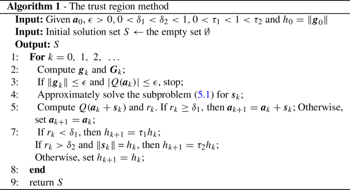
The ratio $r_{k}$ is an indicator for expanding and contracting the trust region. If $r_{k}$ is negative, the current value of $Q({\varvec{a}}_{k})$ is less than the new objective value $Q({\varvec{a}}_{k} + {\varvec{s}}_{k})$, consequently the step should be rejected. If $r_{k}$ is close to 1, it means there is a good agreement between the model $q^{(k)}$ and the objective function Q over this step, we can expand the trust region for the next iteration. If $r_{k}$ is close to zero, the trust region should be contracted. Otherwise, we do not alter the trust region at the next iteration. Moreover, the process is also summarized in the following algorithm 1.

For simplicity, in general we choose $\epsilon = 10^{-13}, \delta _1 = 0.25, \delta _2 = 0.75, \tau _1 = 0.5,$ and $\tau _2 = 2$ throughout the paper. Moreover, in the Algorithm 1 (see Line 4), the subproblem (5.1) needs to be solved. Here the so-called dogleg method (see [11, 26]) is used to solve it, and the process is as follows: Let $s:= {\varvec{a}}_{k} - d_{k}{\varvec{g}}_{k}$, and substituting it into (5.1) yields

$$\begin{aligned} q^{(k)}({\varvec{a}}_{k} - d_{k} {\varvec{g}}_{k}) = Q({\varvec{a}}_{k}) - d_{k}\Vert {\varvec{g}}_{k}\Vert ^{2}_2 + \frac{1}{2}d^2_{k} {\varvec{g}}^{\top }_{k}{\varvec{G}}_{k}{\varvec{g}}_{k}. \end{aligned}$$

Based on the exact line search, the step size $d_{k}$ becomes

$$\begin{aligned} d_{k} = \frac{\Vert {\varvec{g}}_{k}\Vert ^{2}_2}{{\varvec{g}}^{\top }_{k}{\varvec{G}}_{k}{\varvec{g}}_{k}}. \end{aligned}$$

Consequently the corresponding step along the steepest descent direction is

$$\begin{aligned} {\varvec{s}}^C_{k} = - d_{k}{\varvec{g}}_{k} = -\frac{{\varvec{g}}^{\top }_{k}{\varvec{g}}_{k}}{{\varvec{g}}^{\top }_{k}{\varvec{G}}_{k}{\varvec{g}}_{k}}{\varvec{g}}_{k}. \end{aligned}$$

On the other hand, the Newtonian step is

$$\begin{aligned} {\varvec{s}}^{N}_{k} = -{\varvec{G}}^{-1}_{k}{\varvec{g}}_{k}. \end{aligned}$$

If $\Vert {\varvec{s}}^{C}_{k}\Vert _{2} = \Vert d_{k}{\varvec{g}}_{k}\Vert _{2} \ge h_{k}$, the solution of (5.1) can be obtained, i.e.,

$$\begin{aligned} {\varvec{s}}_{k} = -\frac{{\varvec{g}}_{k}}{\Vert {\varvec{g}}_{k}\Vert _2}h_{k}, \end{aligned}$$

(5.3)

which leads to ${\varvec{a}}_{k+1} = {\varvec{a}}_{k} + {\varvec{s}}_{k}$. If $\Vert {\varvec{s}}^{C}_{k}\Vert _2 < h_{k}$ and $\Vert {\varvec{s}}^{N}_{k}\Vert _2 > h_{k}$, a dogleg path consisting of two line segments is used to approximate ${\varvec{s}}$ in (5.1), i.e.,

$$\begin{aligned} {\varvec{s}}_{k}(\lambda ) = {\varvec{s}}^{C}_{k} + \lambda ({\varvec{s}}^{N}_{k} - {\varvec{s}}^{C}_{k}),\quad 0 \le \lambda \le 1. \end{aligned}$$

(5.4)

Obviously, when $\lambda = 0$, ${\varvec{s}}_{k}(\lambda )$ reduces to the steepest descent direction. While $\lambda = 1$, it becomes the Newtonian direction. To exactly obtain $\lambda$ in (5.4), we will solve the following equation:

$$\begin{aligned} \Vert {\varvec{s}}^{C}_{k} + \lambda ({\varvec{s}}^{N}_{k} - {\varvec{s}}^{C}_{k})\Vert _2 = h_{k}. \end{aligned}$$

As a result, we have

$$\begin{aligned} {\varvec{a}}_{k+1} = {\varvec{a}}_{k} + {\varvec{s}}_{k}(\lambda ) = {\varvec{a}}_{k} + {\varvec{s}}^{C}_{k} + \lambda ({\varvec{s}}^{N}_{k} - {\varvec{s}}^{C}_{k}), \end{aligned}$$

Otherwise, we choose

$$\begin{aligned} {\varvec{s}}_{k} = {\varvec{s}}^{N}_{k} = -{\varvec{G}}^{-1}_{k}{\varvec{g}}_{k}. \end{aligned}$$

(5.5)

In summary, with (5.3), (5.4) and (5.5), the solution ${\varvec{s}}_{k}$ in (5.1) becomes

$$\begin{aligned} {\varvec{s}}_{k}={\left\{ \begin{array}{ll}-\frac{{\varvec{g}}_{k}}{\Vert {\varvec{g}}_{k}\Vert _2} h_{k}, &{} \text {if}\;\; \Vert {\varvec{s}}^{C}_{k}\Vert _{2} \ge h_{k}, \quad \quad \quad \quad \quad \quad \quad \quad \quad \quad \quad (\text {I}) \\ {\varvec{s}}^{C}_{k} + \lambda ({\varvec{s}}^{N}_{k} - {\varvec{s}}^{C}_{k}), &{} \text {if}\;\; \Vert {\varvec{s}}^{C}_{k} \Vert _{2}< h_{k}\;\; \text {and}\;\; \Vert {\varvec{s}}^{N}_{k}\Vert _{2} > h_{k}, \quad \quad \quad (\text {II}) \\ -{\varvec{G}}^{-1}_{k}{\varvec{g}}_{k}, &{} \text {if}\;\; \Vert {\varvec{s}}^{C}_{k}\Vert _{2} < h_{k}\;\; \text {and}\;\; \Vert {\varvec{s}}^{N}_{k}\Vert _{2} \le h_{k}. \quad \quad \quad (\text {III}) \end{array}\right. } \end{aligned}$$

(5.6)

Fig. 18

Exact trajectory and dogleg approximation

Next, we remark the trust region method for solving nonlinear algebraic system (2.5). As mentioned in [26], the trust region enjoys the desirable global convergence with a local superlinear rate of convergence as follows.

Theorem 5.1

Assume that

• (i) the function $Q({\varvec{{a}}})$ is bounded below on the level set

  $$\begin{aligned} H := \{{\varvec{{a}}}\in R^{n}\; :\; Q({\varvec{{a}}}) \le Q({\varvec{{a}}}_{0})\}, \quad \forall \, {\varvec{{a}}}_{0}\in \mathbb R^n, \end{aligned}$$

  (5.7)

  and is Lipschitz continuously differentiable in H; 

• (ii) the Hessian matrixes $G({\varvec{{x}}}^{(k)})$ are uniformly bounded in 2-norm, i.e., $\Vert G({\varvec{{a}}}_{k})\Vert \le \beta$ for any k and some $\beta >0$.

If ${\varvec{g}}({\varvec{{a}}}_{k}) \ne {\varvec{0}}$, then

$$\begin{aligned} \lim _{k \rightarrow \infty }\inf \Vert {\varvec{g}}({\varvec{{a}}}_{k})\Vert = 0. \end{aligned}$$

(5.8)

Moreover, if ${\varvec{g}}({\varvec{{a}}}^{*}) = {\varvec{0}}$, and ${\varvec{G}}({\varvec{{a}}}^{*})$ is positive definite, then the convergence rate of the trust region method is quadratic.

Remark 5.1

When k is large enough, the trust region method becomes the Newtonian iteration. As a result, it has the same convergence rate as the Newtonian method. $\square$

Remark 5.2

In practice, the gradient and Hessian matrices might be appropriately approximated by some numerical means. We refer to Zhang et al. [37] for such derivative-free methods for (2.6) with $\varvec{f}$ being twice continuously differentiable, but none of their first-order or second-order derivatives being explicitly available. $\square$

References

Allgower, E.L., Sommese, A.J., Bates, D.J., Wampler, C.W.: Solution of polynomial systems derived from differential equations. Computing 76, 1–10 (2006)
Allgower, E.L., Cruceanu, S.G., Tavener, S.: Application of numerical continuation to compute all solutions of semilinear elliptic equations. Adv. Geom. 76, 1–10 (2009)
Alpert, B.K., Rokhlin, V.: A fast algorithm for the evaluation of legendre expansions. SIAM J. Sci. Stat. Comput. 12, 158–179 (1991)
Chen, C.M., Xie, Z.Q.: Search extension method for multiple solutions of a nonlinear problem. Comput. Math. Appl. 47, 327–343 (2004)
Choi, Y.S., McKenna, P.J.: A mountain pass method for the numerical solution of semilinear elliptic problems. Nonlinear Anal. 20, 417–437 (1993)
Davis, H.T.: Introduction to nonlinear differential and integral equations. US Atomic Energy Commission (1960)
Ding, Z.H., Costa, D., Chen, G.: A high-linking algorithm for sign-changing solutions of semilinear elliptic equations. Nonlinear Anal. 38, 151–172 (1999)
Du, Q., Zhang, L., Zheng, Z.Z.: Optimization-based shrinking dimer method for finding transition states. SIAM J. Sci. Comput. 38, A528–A544 (2016)
Farrell, P.E., Birkisson, A., Funke, S.W.: Deflation techniques for finding distinct solutions of nonlinear partial differential equations. SIAM J. Sci. Comput. 37, A2026–A2045 (2015)
Frisch, U., Matarrese, S., Mohayaee, R., Sobolevski, A.: A reconstruction of the initial conditions of the universe by optimal mass transportation. Nature 417, 260–262 (2002)
Gould, N., Sainvitu, C., Toint, P.L.: A filter-trust-region method for unconstrained optimization. SIAM J. Optim. 16, 341–357 (2006)
Hale, N., Townsend, A.: A fast, simple and stable Chebyshev–Legendre transform using an asymptotic formula. SIAM J. Sci. Comput. 36, A148–A167 (2014)
Hao, W., Lee, S., Lee, Y.J.: Companion-based multi-level finite element method for computing multiple solutions of nonlinear differential equations. arXiv preprint arXiv:2305.04162 (2023)
Hao, Wenrui, Xue, Chuan: Spatial pattern formation in reaction-diffusion models: a computational approach. J. Math. Biol. 80, 521–543 (2020)
Hao, W.R., Hauenstein, J.D., Hu, B., Sommese, A.J.: A bootstrapping approach for computing multiple solutions of differential equations. J. Comput. Appl. Math. 258, 181–190 (2014)
Hao, Wenrui, Hesthaven, Jan, Lin, Guang, Zheng, Bin: A homotopy method with adaptive basis selection for computing multiple solutions of differential equations. J. Sci. Comput. 82, 1–17 (2020)
Hao, W.R., Zhao, X.Y.E., Chen, L.Q., Zhao, Y.X.: Bifurcation analysis reveals solution structures of phase field models. Commun. App. Math. Comput. 6, 64–89 (2024)
Li, Y.X., Zhou, J.X.: A minimax method for finding multiple critical points and its applications to semilinear pdes. SIAM J. Sci. Comput. 23, 840–865 (2001)
Li, Z.X., Yang, Z.H., Zhu, H.I.: Bifurcation method for solving multiple positive solutions to Henon equation. Sci. China Ser. 37, 1417–1428 (2007)
Li, L., Wang, L.L., Li, H.Y.: An efficient spectral trust-region deflation method for multiple solutions. J. Sci. Comput. 32, 1–23 (2023)
McKenna, P.J., Breuer, B., Plum, M.: Multiple solutions for a semilinear boundary value problem: a computational multiplicity proof. J. Differ. Equ. 195, 243–269 (2003)
Natarajan, T., Ahmed, N., Rao, K.R.: Discrete cosine transform. IEEE Trans. Comput. 100, 90–93 (1974)
Nocedal, J., Wright, S.J.: Numerical Optimization, vol. 25. Springer Series in Operations Research (1999)
Shen, J., Tang, T., Wang, L.L.: Spectral Methods: Algorithms, Analysis and Applications, vol. 41. Springer, Berlin (2011)
Steidl, G., Potts, D., Tasche, M.: Fast algorithms for discrete polynomial transforms. Math. Comput. 67, 1577–1590 (1998)
Sun, W.Y., Yuan, Y.X.: Optimization Theory and Methods: Nonlinear Programming, vol. 1. Springer, Berlin (2006)
Tadmor, E.: A review of numerical methods for nonlinear partial differential equations. Bull. Am. Math. Soc. 49, 507–554 (2012)
Trefethen, L.N.: Spectral Methods in MATLAB, vol. 41. Tsinghua University Press, Beijing (2011)
Wang, Y., Hao, W., Lin, G.: Two-level spectral methods for nonlinear elliptic equations with multiple solutions. SIAM J. Sci. Comput. 40, B1180–B1205 (2018)
Xie, Z.Q. Liu, W., Yuan, Y.J.: A constrained gentlest ascent dynamics and its applications to find excited states of Bose–Einstein condensates. https://arxiv.org/pdf/2209.04684v1
Xie, Z.Q., Chen, C.M., Xu, Y.: An improved search-extension method for computing multiple solutions of semilinear PDEs. IMA J. Numer. Anal. 25, 549–576 (2005)
Yang, Z.H., Li, Z.X., Zhu, H.L.: Bifurcation method for solving multiple positive solutions to boundary value problem of henon equation on unit disk. Comput. Math. Appl. 62, 3775–3784 (2011)
Yao, X.D., Zhou, J.X.: A minimax method for finding multiple critical points in banach spaces and its application to quasi-linear elliptic PDEs. SIAM J. Sci. Comput. 26, 1796–1809 (2005)
Yao, X.D., Zhou, J.X.: Numerical methods for computing nonlinear eigenpairs: Part I. Iso-Homogeneous cases. SIAM J. Sci. Comput. 29, 1355–1374 (2007)
Yao, X.D., Zhou, J.X.: Numerical methods for computing nonlinear eigenpairs: Part II. Non-Iso-Homogeneous cases. SIAM J. Sci. Comput 30, 937–956 (2008)
Zhang, J.Y., Du, Q.: Shrinking dimer dynamics and its applications to saddle point search. SIAM J. Numer. Anal. 50, A1899–A1921 (2012)
Zhang, H., Andrew, R., Scheinberg, K.: A derivative-free algorithm for least-squares minimization. SIAM J. Optim. 20, 3555–3576 (2010)
Zhang, X.P., Zhang, J.T., Yu, B.: Eigenfunction expansion method for multiple solutions of semilinear elliptic equations with polynomial nonlinearity. SIAM J. Numer. Anal. 51, 2680–2699 (2013)
Zhang, L., Yin, J.Y., Zhang, P.W.: High-index optimization-based shrinking dimer method for finding high-index saddle points. SIAM J. Sci. Comput. 6, A3576–A3595 (2019)
Zhou, J.X.: Instability analysis of saddle points by a local minimax method. Math. Comput. 74, 1391–1411 (2004)
Zhou, X.: The gentlest ascent dynamics. Nonlinearity 24, 1831–1842 (2011)
Funding
This work is partially supported by the the National Natural Science Foundations of China (Nos. 11871455, 12131005).
Author information
Authors and Affiliations
Corresponding author
Ethics declarations
Conflict of interest
The authors have no relevant financial interest to disclose.
Additional information
Publisher's Note
Springer Nature remains neutral with regard to jurisdictional claims in published maps and institutional affiliations.