
Abstract
This paper considers a model in which agents have heterogeneous preferences over labour and consumption. Additionally, they also differ in their earning skills, which are a function of both an innate ability and an early investment decision. In this framework we axiomatically derive a social ordering function that, besides compensating agents for their unequal productivities, grants a fresh start to those who regret their initial choices. Next, by assuming a second-best context we characterise the income tax scheme that satisfies this social ordering. This analysis permits us to present an explicit criterion for the assessment of social welfare under different tax policies. We obtain that the optimal scheme aims to compensate those endowed with the lowest marginal productivity. More importantly, on account of the forgiveness ideal positive social marginal weights are assigned to those who earn the lowest income levels, something that induces a progressivity tendency at the bottom of the earnings distribution.
Article PDF
Notes
\({T^{s}_{f}}(x^{\tilde {s}}_{f^{\prime }})\) represents the well-being level that an agent endowed with \(s^{\alpha }\in \{s_{L}^{\alpha },s_{H}^{\alpha }\}\) and ex post preferences \(R_{f}\in \mathcal {R}\) gets from a bundle \(x^{s^{\prime }}_{f^{\prime }}\in X\), which was chosen by someone who has a production skill \(\tilde {s}^{\alpha }\in \{s_{L}^{\alpha },s_{H}^{\alpha }\}\) and ex ante preferences \(R_{f^{\prime }}\in \mathcal {R}\).
References
Arneson, R.J.: Equality and equal opportunity for welfare. Philos. Stud. 56(1), 77–93 (1989)
Arrow, K.J.: Social Choice an Individual Values. Wiley, New York (1951)
Bossert, W., Fleurbaey, M., Van de Gaer, D.: Responsibility, talent, and compensation: A second-best analysis. Rev. Econ. Des. 4(1), 35–55 (1999)
Bovenberg, A.L., Jacobs, B.: Redistribution and education subsidies are siamese twins. J. Public Econ. 89(11), 2005–2035 (2005)
Calo-Blanco, A.: Fairness, freedom, and forgiveness in health care. Soc. Choice Welf. 43(1), 141–151 (2014)
Calo-Blanco, A.: Fair compensation with different social concerns for forgiveness. Rev. Econ. Des. 20(1), 39–56 (2016)
Calo-Blanco, A.: Health, responsibility and taxation with a fresh start. SERIEs 8(2), 177–199 (2017)
Cohen, G.A.: On the currency of egalitarian justice. Ethics 99(4), 906–944 (1989)
D’Aspremont, C., Gevers, L.: Equity and the informational basis of collective choice. Rev. Econ. Stud. 44(2), 199–209 (1977)
Dworkin, R.: What is equality? part 1: Equality of welfare. Philos. Public Aff. 10(3), 185–246 (1981a)
Dworkin, R.: What is equality? part 2: Equality of resources. Philos. Public Aff. 10(4), 283–345 (1981b)
Dworkin, R.: Sovereign Virtue: The Theory and Practice of Equality. Stanford series in philosophy. Harvard University Press, Cambridge (2000)
Dworkin, R.: Sovereign virtue revisited. Ethics 113(1), 106–143 (2002)
Findeisen, S., Sachs, D.: Education and optimal dynamic taxation: The role of income-contingent student loans. J. Public Econ. 138, 1–21 (2016)
Fleurbaey, M.: Freedom with forgiveness. Polit/ Philos. Econ. 4(1), 29–67 (2005)
Fleurbaey, M.: Fairness, Responsibility, and Welfare. Oxford University Press, Oxford (2008)
Fleurbaey, M., Maniquet, F.: Fair social orderings when agents have unequal production skills. Soc. Choice Welf. 24(1), 93–127 (2005)
Fleurbaey, M., Maniquet, F.: Fair income tax. Rev. Econ. Stud. 73(1), 55–83 (2006)
Fleurbaey, M., Maniquet, F.: A Theory of Fairness and Social Welfare. Cambridge University Press, Cambridge (2011)
Fleurbaey, M., Maniquet, F.: Optimal income taxation theory and principles of fairness. J. Econ. Lit. 56(3), 1029–1079 (2018)
Fleurbaey, M., Valletta, G.: Fair optimal tax with endogenous productivities. J. Public Econ. Theory 20(6), 849–873 (2018)
Hansson, B.: The independence condition in the theory of social choice. Theor. Decis. 4(1), 25–49 (1973)
Jacobs, B., Bovenberg, A.L.: Optimal taxation of human capital and the earnings function. J. Public Econ. Theory 13(6), 957–971 (2011)
Luttens, R.I., Ooghe, E.: Is it fair to ‘make work pay’? Economica 74(296), 599–626 (2007)
Mirrlees, J.A.: An exploration in the theory of optimum income taxation. Rev. Econ. Stud. 38(2), 175–208 (1971)
Pazner, E.A.: Equity, nonfeasible alternatives and social choice: a reconsideration of the concept of social welfare . In: Laffont, J.J. (ed.) Aggregation and Revelation of Preferences. North-Holland, Amsterdam (1979)
Rawls, J.: A Theory of Justice. Harvard University Press, Cambridge (1971)
Roemer, J.E.: Equality of Opportunity. Harvard University Press, Cambridge (1998)
Saez, E., Stantcheva, S.: Generalized social marginal welfare weights for optimal tax theory. Am. Econ. Rev. 106(1), 24–45 (2016)
Schokkaert, E., de gaer, D.V., Vandenbroucke, F., Luttens, R.I.: Responsibility sensitive egalitarianism and optimal linear income taxation. Math. Soc. Sci. 48(2), 151–182 (2004)
Stantcheva, S.: Optimal taxation and human capital policies over the life cycle. J. Polit. Econ. 125(6), 1931–1990 (2017)
Valletta, G.: Health, fairness and taxation. Soc. Choice Welf. 43(1), 101–140 (2014)
Acknowledgements
I would like to thank Mar Calo, José Gabriel Romero, José A. Novo-Peteiro and the participants to seminars and conferences in Bilbao, Seville and Madrid for their helpful comments. Financial support from the Spanish Ministry of Economy and Competitiveness, under projects ECO2017-83069-P and ECO2014-57413-P, is gratefully acknowledged. Funding for open access charge: Universidade da Coruña/CISUG. The usual disclaimer applies.
Funding
Open Access funding provided thanks to the CRUE-CSIC agreement with Springer Nature.
Author information
Authors and Affiliations
Corresponding author
Additional information
Publisher’s note
Springer Nature remains neutral with regard to jurisdictional claims in published maps and institutional affiliations.
Appendices
Appendix A: Proof of Theorem 1
In order to prove this theorem we first need to introduce the following lemma:
Lemma 1
If a social ordering function satisfies Strong Pareto, Independence and Equal Preferences Transfer, then for all \(e\in \mathcal {E}\) and \(z_{N},z^{\prime }_{N}\in Z^{n}\), if there exist j,k ∈ N with \({R^{p}_{j}}={R^{p}_{k}}\) such that:
and \(z_{i}=z^{\prime }_{i}\) for all i≠j,k, then \(z_{N}\text {\textbf {P}}(e)z^{\prime }_{N}\).
For proof of Lemma 1 see Fleurbaey and Maniquet (2006).
Let us now turn to prove Theorem 1. The proof is split in three steps.
- Step 1 : :
-
For any \(e\in \mathcal {E}\), let us consider two individuals j,k ∈ N and two allocations \(z_{N},z^{\prime }_{N}\in Z^{n}\) such that, without loss of generality, \(T_{k}(z_{k},{R^{p}_{k}})=T_{j}(z^{\prime }_{j},{R^{p}_{j}})>T_{k}(z^{\prime }_{k},{R^{p}_{k}})=T_{j}(z_{j},{R^{p}_{j}})\), and \(z_{i}=z^{\prime }_{i}\) for all i≠j,k. We need to prove that it must be the case that \(z_{N}\textbf {I}(e)z^{\prime }_{N}\). Opposite to the desired result, let us assume that \(z_{N}\textbf {P}(e)z^{\prime }_{N}\).
Let us now introduce two additional individuals b,m such that \(s_{b}^{\alpha }=s_{m}^{\alpha }=s_{L}^{\alpha }\), \({R^{p}_{b}}={R^{p}_{j}}\in \mathcal {R}\) and \({R^{p}_{m}}={R^{p}_{k}}\in \mathcal {R}\). Let us also assume that there exist \(z_{b},z^{\prime }_{b},z^{\prime \prime }_{b},z^{\prime \prime \prime }_{b},\) \(z_{m},z^{\prime }_{m},z^{\prime \prime }_{m},z^{\prime \prime \prime }_{m}\in Z\) such that:
$$ \begin{array}{c} T_{b}(z_{b},{R^{p}_{b}})=T_{m}(z^{\prime}_{m},{R^{p}_{m}})=T_{k}(z_{k},{R^{p}_{k}})>T_{b}(z^{\prime}_{b},{R^{p}_{b}})=T_{m}(z_{m},{R^{p}_{m}})=T_{j}(z_{j},{R^{p}_{j}}), \\ z_{b}=z^{\prime}_{j}, \ z^{\prime}_{b}=z_{j}, \ z_{m}=z^{\prime}_{k}, \ z^{\prime}_{m}=z_{k}, \\ z^{\prime\prime}_{b}{I^{p}_{b}}z_{b}, \ z^{\prime\prime\prime}_{b}{I^{p}_{b}}z^{\prime}_{b}, \ z^{\prime\prime}_{m}{I^{p}_{m}}z_{m}, \ z^{\prime\prime\prime}_{m}{I^{p}_{m}}z^{\prime}_{m}, \\ z^{\prime\prime}_{b},z^{\prime\prime\prime}_{b}\in Z({R^{p}_{b}},s_{b}^{\alpha}), \ z^{\prime\prime}_{m},z^{\prime\prime\prime}_{m}\in Z({R^{p}_{m}},s_{m}^{\alpha}), \end{array} $$where for any \(R\in \mathcal {R}\) and \(s^{\alpha }\in \mathcal {S}\), and for all \(t\in \mathbb {R}\), the set \(Z(R,s^{\alpha })=\{z\in Z\left | z\in \max \limits \right |_{R} B(t,s^{\alpha })\}\) gathers all the bundles that maximise \(R\in \mathcal {R}\) for any budget set which is defined by sα.
According to the initial assumptions, if we apply Separation we can add identical individuals in both allocations without altering social preferences over them, that is, \((z_{N},z_{b},z_{m})\textbf {P}(e)(z^{\prime }_{N},z_{b},z_{m})\). Combining Strong Pareto (which implies Pareto Indifference) and Equal Preferences Transfer twice we can induce the following relations: \((z_{-\{k\}},z^{\prime }_{k},z_{b},z^{\prime }_{m})\textbf {I}(e)(z,z_{b},z_{m})\) and \((z_{-\{j,k\}},z^{\prime }_{j},z^{\prime }_{k},z^{\prime }_{b},z^{\prime }_{m})\textbf {I}(e)(z_{-\{k\}},z^{\prime }_{k},z_{b},z^{\prime }_{m})\). If we apply Strong Pareto \((z^{\prime }_{N},z^{\prime }_{b},z^{\prime }_{m})\textbf {I}(e)(z_{-\{j,k\}},z^{\prime }_{j},z^{\prime }_{k},z^{\prime }_{b},z^{\prime }_{m})\). Using Transitivity we have that \((z^{\prime }_{N},z^{\prime }_{b},z^{\prime }_{m})\textbf {P}(e)(z^{\prime }_{N},z_{b},z_{m})\), and according to Separation we can state that \((z^{\prime }_{b},z^{\prime }_{m})\textbf {P}(e)(z_{b},z_{m})\). However, if we apply \(s_{L}^{\alpha }\)-Skill Transfer and Strong Pareto axioms it is straightforward to obtain first \((z^{\prime \prime }_{b},z^{\prime \prime }_{m})\textbf {I}(e)(z^{\prime \prime \prime }_{b},z^{\prime \prime \prime }_{m})\), and next that \((z_{b},z_{m})\textbf {I}(e)(z^{\prime }_{b},z^{\prime }_{m})\), which yields the desired contradiction.
- Step 2 : :
-
For any \(e\in \mathcal {E}\), let us consider, without loss of generality, two allocations \(z_{N},z^{\prime }_{N}\in Z^{n}\) and two individuals j,k ∈ N such that \(T_{j}(z^{\prime }_{j},{R^{p}_{j}})<T_{k}(z_{k},{R^{p}_{k}})<T_{j}(z_{j},{R^{p}_{j}})<T_{k}(z^{\prime }_{k},{R^{p}_{k}})\), and \(z_{i}=z^{\prime }_{i}\) for all i≠j,k. We need to prove that \(z_{N}\textbf {P}(e)z^{\prime }_{N}\). Opposite to the desired result, let us assume that \(z^{\prime }_{N}\textbf {R}(e)z_{N}\).
Let us now introduce two additional individuals b,m such that \(s_{b}^{\alpha }=s_{m}^{\alpha }=s_{L}^{\alpha }\), \({R^{p}_{b}}={R^{p}_{j}}\in \mathcal {R}\) and \({R^{p}_{m}}={R^{p}_{k}}\in \mathcal {R}\). Let us also assume that there exist \(z^{\prime \prime }_{j},z^{\prime \prime }_{k},z^{\prime \prime }_{b},z^{\prime \prime }_{m}\in Z\), \(z_{b},z^{\prime }_{b}\in Z({R^{p}_{b}},s_{b}^{\alpha })\) and \(z_{m},z^{\prime }_{m}\in Z({R^{p}_{m}},s_{m}^{\alpha })\) such that:
$$ \begin{array}{c} z_{j}{P^{p}_{j}}z_{b}{P^{p}_{b}}z_{b}^{\prime}{P^{p}_{b}}z_{b}^{\prime\prime}{P^{p}_{b}}z_{j}^{\prime\prime}{P^{p}_{j}}z_{j}^{\prime}, \\ z_{k}^{\prime}{P^{p}_{k}}z_{k}{P^{p}_{k}}z^{\prime\prime}_{k}{P^{p}_{k}}z_{m}^{\prime}{P^{p}_{m}}z_{m}^{\prime\prime}{P^{p}_{m}}z_{m}. \end{array} $$Moreover, there exists \(\delta \in \mathbb {R}_{++}\) such that:
$$ \begin{array}{c} c^{\prime}_{m}-(s_{m}^{\alpha^{\prime}_{m}}\ell^{\prime}_{m}-\epsilon\alpha^{\prime}_{m})-\delta=c_{m}-(s_{m}^{\alpha_{m}}\ell_{m}-\epsilon\alpha_{m})> \\ c_{b}-(s_{b}^{\alpha_{b}}\ell_{b}-\epsilon\alpha_{b})=c^{\prime}_{b}-(s_{b}^{\alpha^{\prime}_{b}}\ell^{\prime}_{b}-\epsilon\alpha^{\prime}_{b})+\delta. \end{array} $$According to the initial assumptions and the Separation axiom we have that \((z^{\prime }_{N},z_{b},\) zm)R(e)(zN,zb,zm). Applying Lemma 1 twice we obtain that \((z^{\prime }_{-\{j,k\}},z^{\prime \prime }_{j},z^{\prime \prime }_{k},z^{\prime \prime }_{b},z^{\prime \prime }_{m})\) \(\textbf {P}(e)(z^{\prime }_{N},z_{b},z_{m})\). Additionally, Strong Pareto implies that \((z^{\prime }_{-\{j,k\}},z_{j},z_{k},z^{\prime \prime }_{b},z^{\prime \prime }_{m})\textbf {P}(e)\) \((z^{\prime }_{-\{j,k\}},z^{\prime \prime }_{j},z^{\prime \prime }_{k},z^{\prime \prime }_{b},z^{\prime \prime }_{m})\). Finally, by Pareto Indifference, Transitivity and Separation we have that \((z^{\prime \prime }_{b},z^{\prime \prime }_{m})\textbf {P}(e)(z_{b},z_{m})\). However, if we apply Strong Pareto we get that \((z^{\prime }_{b},z^{\prime }_{m})\textbf {P}(e)(z^{\prime \prime }_{b},z^{\prime \prime }_{m})\), and according to \(s_{L}^{\alpha }\)-Skill Transfer we have that (zb,zm)R(e) \((z^{\prime }_{b},z^{\prime }_{m})\). Transitivity induces then that \((z_{b},z_{m})\textbf {P}(e)(z^{\prime \prime }_{b},z^{\prime \prime }_{m})\), which yields the desired contradiction.
Finally, we can design a series of allocations that would allow us to prove that whenever there exist \(z_{N},z^{\prime }_{N}\in Z^{n}\) such that \(\min \limits _{i\in N}T_{i}(z_{i},{R^{p}_{i}})>\min \limits _{i\in N}T_{i}(z^{\prime }_{i},{R^{p}_{i}})\Rightarrow z_{N}\textbf {P}(e)z^{\prime }_{N}\). Let us take then two allocations \(z_{N},z^{\prime }_{N}\in Z^{n}\) such that \(\min \limits _{i\in N}T_{i}(z_{i},{R^{p}_{i}})>\min \limits _{i\in N}T_{i}(z^{\prime }_{i},{R^{p}_{i}})\).
Because of the strict monotonicity of the preferences, one can find two allocations \(x_{N},x^{\prime }_{N}\in Z^{n}\) such that for all i ∈ N we have \(T_{i}(z_{i},{R^{p}_{i}})>T_{i}(x_{i},{R^{p}_{i}})\) and \(T_{i}(x^{\prime }_{i},{R^{p}_{i}})>T_{i}(z^{\prime }_{i},{R^{p}_{i}})\). Moreover, there exists i0 such that for all i≠i0:
$$ T_{i}(x^{\prime}_{i},{R^{p}_{i}})>T_{i}(x_{i},{R^{p}_{i}})>T_{i_{0}}(x_{i_{0}},R^{p}_{i_{0}})>T_{i_{0}}(x^{\prime}_{i_{0}},R^{p}_{i_{0}}). $$Let Q = N ∖{i0} and let us assume a sequence of allocations \(({x_{N}^{q}})_{1 \leq q \leq |Q|+1}\) such that:
$$ \left. \begin{array}{c} T_{i}({x_{i}^{q}},{R^{p}_{i}})=T_{i}(x^{\prime}_{i},{R^{p}_{i}}), \ \ \ \forall i \in Q: \ i \geq q, \\ T_{i}({x_{i}^{q}},{R^{p}_{i}})=T_{i}(x_{i},{R^{p}_{i}}), \ \ \ \forall i \in Q: \ i < q, \end{array} \right. $$whereas,
$$ T_{i_{0}}(x_{i_{0}},R^{p}_{i_{0}})=T_{i_{0}}(x^{|Q+1|}_{i_{0}},R^{p}_{i_{0}})>T_{i_{0}}(x^{|Q|}_{i_{0}},R^{p}_{i_{0}})>\ldots> T_{i_{0}}(x^{1}_{i_{0}},R^{p}_{i_{0}})=T_{i_{0}}(x^{\prime}_{i_{0}},R^{p}_{i_{0}}). $$This implies that \(T_{i_{0}}(x_{i_{0}}^{q},R^{p}_{i_{0}})<T_{i_{0}}(x_{i_{0}}^{q+1},R^{p}_{i_{0}})<T_{q}(x_{q}^{q+1},{R^{p}_{q}})<T_{q}({x_{q}^{q}},{R^{p}_{q}})\), while for all j≠q,i0, we have that \(T_{j}({x_{j}^{q}},{R^{p}_{j}})=T_{j}(x_{j}^{q+1},{R^{p}_{j}})\). As we have previously proved, it must be the case that \(x_{N}^{q+1}\textbf {P}(e){x_{N}^{q}}\), ∀q ∈ Q. According to the initial assumptions, by Strong Pareto we have that \(z_{N}\textbf {P}(e)x_{N}^{|Q|+1}\) and \({x_{N}^{1}}\textbf {P}(e)z^{\prime }_{N}\). Finally, by Transitivity we have that \(z_{N}\textbf {P}(e)z^{\prime }_{N}\).
- Step 3 : :
-
In this last step of the proof we extend our result in order to meet the leximin criterion, that is, for any \(e\in \mathcal {E}\) and \(z_{N},z^{\prime }_{N}\in Z^{n}\) we have to show that \((T_{i}(z_{i},{R^{p}_{i}}))_{i\in N}\) \(>_{\text {lex}}(T_{i}(z^{\prime }_{i},{R^{p}_{i}}))_{i\in N}\Rightarrow z_{N}\textbf {P}(e)z^{\prime }_{N}\). Without loss of generality, let us assume that there exist j,k ∈ N such that \(\min \limits _{i\in N}T_{i}(z_{i},{R^{p}_{i}})=T_{j}(z_{j},{R^{p}_{j}})=T_{k}(z^{\prime }_{k},{R^{p}_{k}})=\min \limits _{i\in N}T_{i}\) \((z^{\prime }_{i},{R^{p}_{i}})\). Additionally, we consider that \(\min \limits _{i\in N}T_{i}(x_{i},{R^{p}_{i}})>\min \limits _{i\in N}T_{i}(x^{\prime }_{i},{R^{p}_{i}})\), where \(x_{N},x^{\prime }_{N}\in Z^{n-1}\) are the allocations that are constructed as the original ones but removing, in each one of them, the individual with the lowest \(s_{-}^{\alpha }\)-Implicit Transfer. By Strong Pareto and repeated application of Step 1 we have that \(\overline {z}_{N}\textbf {I}(e)z_{N}\), where \(\overline {z}_{N}\) is designed such that the lexicographic values of the implicit transfers in both allocations is the same, that is \((T_{i}(\overline {z}_{i},{R^{p}_{i}}))_{i\in N}=_{\text {lex}}(T_{i}(z_{i},{R^{p}_{i}}))_{i\in N}\), and moreover \(\min \limits _{i\in N}T_{i}(\overline {z}_{i},{R^{p}_{i}})=T_{k}(\overline {z}_{k},{R^{p}_{k}})=T_{k}(z^{\prime }_{k},{R^{p}_{k}})\). Then, by Separation and Step 2 we have that \(\overline {z}_{N}\textbf {P}(e)z^{\prime }_{N}\), and by means of Transitivity we reach the desired result \(z_{N}\textbf {P}(e)z^{\prime }_{N}\).
Appendix B: Proof of Theorem 2
This proof is based on the result obtained by Fleurbaey (2005). Let us start the proof by showing that, for any economy \(e\in \widetilde {\mathcal {E}}\), in any ex post optimal incentive-compatible allocation xN = (yi,ci)i∈N ∈ Xn all resources are exhausted, that is, \({\sum }_{i\in N}\tau (y_{i})=0\). Opposite to the desired result, let us consider an incentive-compatible allocation \(x^{\prime }_{N}=(y^{\prime }_{i},c^{\prime }_{i})_{i\in N}\in X^{n}\) with \({\sum }_{i\in N}\tau (y^{\prime }_{i})>0\).
If \(x^{\prime }_{j}=x^{\prime }_{k}\) for all j,k ∈ N, it is possible to define a parameter δ > 0 such that if we replace the original allocation \(x^{\prime }_{N}\) by \(x^{\delta }_{N}=(y^{\prime }_{i},c^{\prime }_{i}+\delta )_{i\in N}\in X^{n}\), we obtain a new feasible and incentive-compatible allocation in which, because of strict monotonicity, all individuals are better-off.
Let us now deal with the case in which individuals do not have the same bundle, that is, there exist j,k ∈ N such that \(x^{\prime }_{j}\neq x^{\prime }_{k}\). Since the feasible space is defined in terms of pre-tax earnings and final consumption, because of the incentive-compatible constraint the final allocation must be distributed along the unique (net of tax) budget set. Note that due to the monotonicity of the preferences and the incentive-compatible constraint we have to restrict our attention to tax functions such that y − τ(y) is non-decreasing. Hence, those who choose the largest level of income also have the highest consumption. Moreover, due to the assumptions of the model and No Identification, among these agents we can find one endowed with both preferences RF and the highest innate ability.
Therefore, because of the single-crossing property we can use the extra resources to slightly improve the situation of this agent, increasing, this way, social welfare due to the lexicographic condition of the social preferences. Let \({x^{s}_{f}}\in X\) denote the choice of an agent who has a production skill \(s^{\alpha }\in \{s_{L}^{\alpha },s_{H}^{\alpha }\}\) and the ex ante preferences \(R_{f}\in \mathcal {R}\). Then, by increasing the consumption associated with bundle \({x^{H}_{F}}\) social welfare increases. If there exist incentive-compatibility problems with other agents who are indifferent to \({x^{H}_{F}}\), we can always move the bundle along the indifference curve of these individuals, if they share preferences. Note that this movement does not provide the other agents with incentives to change their own choice. As a result of this, in this new feasible allocation incentive-compatibility is still satisfied and social welfare is higher.
Let us now proceed to prove the four different results of Theorem 2.
-
i) For any economy \(e\in \widetilde {\mathcal {E}}\), if all individuals are equal-off in terms of the reference comparable well-being measure, then any j,k ∈ N who share ex post preferences \(R_{f}\in \mathcal {R}\) will have their bundles located in the same indifference curve in space Z. Consequently, in the income-consumption space X their indifference curves have to start from the same point in the vertical axis (zero income point). If these agents are endowed with different production skills, from this point onwards the curve associated with \(\widehat {R}^{H}_{f}\) has to be located to the right of that of \(\widehat {R}^{L}_{f}\). This is so because the high-skilled individual can always get the same (y,c) pair as the low-skilled one by using a lower labour time.
As a result of this, and because of the single-crossing property, to satisfy the incentive-compatible constraints all bundles but \({x_{F}^{H}}\) must be identical and associated with y = 0. Additionally, this zero income point and \({x_{F}^{H}}\) have to be located along the same \(\widehat {R}^{H}_{F}\) indifference curve. Therefore, due to the single-crossing property, the \(s^{\alpha }_{L}\)-Implicit Transfers can never be identical unless all individuals show an extremely low concern for labour.
-
ii) Let us start the proof by considering the group of steady agents (i.e., those who do not regret their initial choice) who are endowed with a good innate ability. By incentive-compatibility they can never be worse-off than the steady bad production skill individuals who have the same concern for labour. Let us now analyse this second group of agents. Due to the incentive-compatible constraint and the single-crossing property, those with \(\widehat {R}^{L}_{f}\neq \widehat {R}^{L}_{1}\) are better-off, or at least equal-off, than the regretful low-skilled agents who choose with preferences \(\widehat {R}^{L}_{f_{1}}\), where \(\widehat {R}^{L}_{f}\succ ^{\ell }\widehat {R}^{L}_{f_{1}}\), and who ex post substitute them for \(\widehat {R}^{L}_{f}\).
Consequently, let us now focus on the set of individuals who regret their initial choice. As regards the high-skilled ones, for any \(R_{f},R_{f_{1}}\in \mathcal {R}\), where \(R_{f}\succ ^{\ell }R_{f_{1}}\), there exists a third type \(R_{f_{2}}\in \mathcal {R}\) with \(R_{f_{2}}\succ ^{\ell }R_{f}\) such that, because of the incentive-compatible constraint and the single-crossing property, \(T^{H}_{f_{2}}({x^{H}_{f}})\geq T^{H}_{f_{2}}(x^{H}_{f_{1}})\).Footnote 1 Note that this argument is valid for all agents but those making their choice with R1. This same line of reasoning can be applied to the bad production skill agents.
Additionally, note that by Assumption 1 we have that \({y^{H}_{1}}\geq {y^{L}_{1}}\) and \({c^{H}_{1}}\geq {c^{L}_{1}}\), where \({y^{s}_{f}}\) (respectively, \({c^{s}_{f}}\)) denotes the income choice (respectively, consumption choice) of an agent who has production skill \(s^{\alpha }\in \{s_{L}^{\alpha },s_{H}^{\alpha }\}\) and ex ante preferences \(R_{f}\in \mathcal {R}\). Therefore, it has to be the case that \({T^{H}_{F}}({x^{H}_{1}})\geq {T^{L}_{F}}({x^{L}_{1}})\).
In consequence, in order to characterise the lowest \(s_{L}^{\alpha }\)-Implicit Transfer we have to focus on the low-skilled individuals with the ex ante preferences \(R_{1}\in \mathcal {R}\). However, because of the single-crossing property, for any \(R_{f}\in \mathcal {R}\) we have either \({T^{L}_{F}}({x^{L}_{1}})\leq {T^{L}_{f}}({x^{L}_{1}})\) or \({T^{L}_{1}}({x^{L}_{1}})\leq {T^{L}_{f}}({x^{L}_{1}})\).
Finally, Fig. 7 depicts two examples in which either \({T^{L}_{1}}({x^{L}_{1}})<{T^{L}_{F}}({x^{L}_{1}})\) or \({T^{L}_{1}}\) \(({x^{L}_{1}})>{T^{L}_{F}}({x^{L}_{1}})\). In both cases all incentive-compatibility constraints are satisfied in such a way that it is not possible to increase social welfare.
Fig. 7 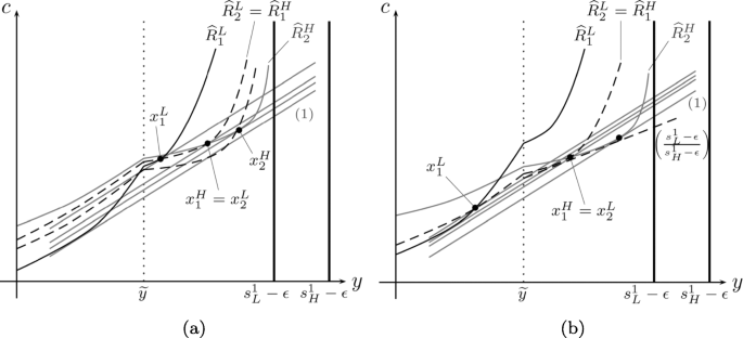
Proof of Theorem 2.ii
-
iii) In order to prove the third point of Theorem 2, let us first show that for every \(R_{f}\in \mathcal {R}\setminus \{R_{F}\}\) one has that \(x^{L}_{f+1}\widehat {I}^{L}_{f+1}{x^{L}_{f}}\).
Opposite to the desired result, let us assume that \(x^{L}_{f+1}\widehat {P}^{L}_{f+1}{x^{L}_{f}}\) for some Rf≠RF. Then, due to the properties of the model we have that \(x^{L}_{f_{1}}\widehat {P}^{L}_{f_{1}}x^{L}_{f_{0}}\) for all f1 > f ≥ f0.
Let us now consider that for every f2 > f there exists f3 > f such that \({x^{L}_{2}}\neq {x^{L}_{3}}\) and \({x^{L}_{2}}\widehat {I}^{L}_{2}{x^{L}_{3}}\). If f2 < f3, by incentive-compatibility we have \({x^{L}_{3}}\neq {x^{L}_{4}}\) and \({x^{L}_{3}}\widehat {I}^{L}_{3}{x^{L}_{4}}\) with f3 < f4, which yields an impossibility since, eventually, it is not possible to obtain the same relation for preferences RF. Note that we may have \({x^{L}_{F}}\widehat {I}^{L}_{F}{x^{H}_{F}}\), with \({x^{L}_{F}}\neq {x^{H}_{F}}\). However, in that case all bundles would be in the \([0,{s_{L}^{1}}-\epsilon ]\) interval, and hence the previous argumentation would lead us to the same difficulty, but including all those endowed with a good production skill. If f2 > f3 a similar impossibility occurs since we are constrained by \(x^{L}_{f_{1}}\widehat {P}^{L}_{f_{1}}{x^{L}_{f}}\).
Therefore, under the previous assumption there exits f2 > f such that for all \(f^{\prime }\neq f_{2}\) we have that \(x^{L}_{f_{2}}\widehat {P}^{L}_{f_{2}}x^{L}_{f^{\prime }}\), with \(x^{L}_{f^{\prime }}\neq x^{L}_{f_{2}}\). Hence, we can slightly increase the tax associated with this bundle, and any other one that is identical, leaving the other choices unchanged. This yields a new incentive-compatible allocation in which some resources are saved without altering the lowest \(s^{\alpha }_{L}\)-Implicit Transfer, which has to be related to a bundle chosen with R1 (see point ii). These resources can be used to increase the minimum equivalent well-being (see Fleurbaey 2005). Note that if both \(x^{L}_{f_{2}}=x^{H}_{f_{2}-1}\) and \(x^{H}_{f_{2}-1}\widehat {I}^{H}_{f_{2}-1}x^{H}_{f_{2}}\) with \(y^{H}_{f_{2}}>{s_{L}^{1}}-\epsilon \), this may prevent us from obtaining the desired result. In such a case we can also increase the tax paid in \(x^{H}_{f_{2}}\), unless we also have that \(x^{H}_{f_{2}}\widehat {I}^{H}_{f_{2}}x^{H}_{f_{2}+1}\). However, this would imply that \(x^{H}_{f^{\prime }}\widehat {P}^{H}_{f^{\prime }}x^{H}_{f^{\prime \prime }}\), with \(y^{H}_{f^{\prime }}>{s_{L}^{1}}-\epsilon \), for all \(f^{\prime }>f_{2}\geq f^{\prime \prime }\), which, as we have previously argued, leads to an impossibility.
As a result of this, for any \(R_{f}\in \mathcal {R}\setminus \{R_{F}\}\) it has to be the case that \(x^{L}_{f+1}\widehat {I}^{L}_{f+1}{x^{L}_{f}}\).
Let us finally consider that for some f < F one has \(\tau ({y^{L}_{f}})>\tau (y^{L}_{f+1})\), where \({y^{L}_{f}}<y^{L}_{f+1}\). Then, since \(x^{L}_{f+1}\widehat {I}^{L}_{f+1}{x^{L}_{f}}\), if we change the bundle \(x^{L}_{f+1}\) by \({x^{L}_{f}}\) we obtain a new allocation that both is incentive-compatible and saves resources. Moreover, the lowest \(s^{\alpha }_{L}\)-Implicit Transfer does not decrease. Consequently, in the optimal allocation one has \(\tau ({y^{L}_{f}})\leq \tau (y^{L}_{f+1})\) for all f < F.
-
iv) Let us finish the proof of Theorem 2 by describing how to compare any two different minimal taxation schemes in terms of social welfare.
For any i ∈ N, the \(s_{L}^{\alpha }\)-Implicit Transfer in the first-best scenario is defined as:
$$ T_{i}(z_{i},{R^{p}_{i}})=\max\{t\in\mathbb{R}\mid\forall(\ell,c)\in Z \ \ \text{s.t.} \ \ c\leq\max\{{s_{L}^{0}}\ell,{s_{L}^{1}}\ell-\epsilon\}+t, \ z_{i}{R^{p}_{i}}(\ell,c)\}, $$which is equivalent to write that:
$$ T_{i}(z_{i},{R^{p}_{i}})=\min\{t\in\mathbb{R}\mid\exists(\ell,c)\in Z \ \ \text{s.t.} \ \ c=\max\{{s_{L}^{0}}\ell,{s_{L}^{1}}\ell-\epsilon\}+t, \ z_{i}{I^{p}_{i}}(\ell,c)\}. $$Since we are analysing the fresh start taxation policy in a second-best scenario, such a measure has to be converted to the non-observable labour space X. Specifically:
$$\begin{array}{ll} T^{s_{i}}_{i}(x_{i},{R^{p}_{i}})&= \min\{t\in\mathbb{R}\mid\exists(y,c)\in X \ \ \text{s.t.} \ \ c=\left( \frac{{s_{L}^{y}}-\epsilon^{y}}{{s^{y}_{i}}-\epsilon^{y}}\right)y+t, \ x_{i}\left( \widehat{I}^{s_{i}}_{i}\right)^{p}(y,c)\} \\ &=\min\left\{c-\left( \frac{{s_{L}^{y}}-\epsilon^{y}}{{s^{y}_{i}}-\epsilon^{y}}\right)y\mid(y,c)\in X, \ x_{i}\left( \widehat{I}^{s_{i}}_{i}\right)^{p}(y,c)\right\}, \end{array}$$which for a low-skilled agent turns into the following expression:
$$ {T^{L}_{i}}(x_{i},{R^{p}_{i}}) =\underset{(y,c)\left( \widehat{I}_{i}^{L}\right)^{p}x_{i}}{\min}(c-y). $$By the second point of Theorem 2 we know that the worst-off individual is a low-skilled agent who either sticks to R1 or changes such preferences for RF, and hence,
$$ \underset{i\in N}{\min}T^{s_{i}}_{i}(x_{i},{R^{p}_{i}}) =\underset{(y,c)\in\widehat{\tau}(y), \ y\leq {s_{L}^{1}}-\epsilon}{\min}(c-y), $$where \(\widehat {\tau }(y)\) is the set of (y,c)-points that envelops the indifference curves of \(\widehat {R}^{L}_{1}\) and \(\widehat {R}^{L}_{F}\) which pass through \({x_{1}^{L}}\), and that are induced by the unique budget set modified by the minimal tax scheme τ(y). Therefore:
$$ \underset{i\in N}{\min}T^{s_{i}}_{i}(x_{i},{R^{p}_{i}})=\underset{y\leq {s_{L}^{1}}-\epsilon}{\min}-\widehat{\tau}(y). $$Finally, for any pair \(x_{N},x^{\prime }_{N}\in X^{n}\) obtained, respectively, with minimal tax schemes τ(y) and \(\tau ^{\prime }(y)\), we know that \(\min \limits _{i}T^{s_{i}}_{i}(x_{i},{R^{p}_{i}})>\min \limits _{i}T^{s_{i}}_{i}(x^{\prime }_{i},{R^{p}_{i}})\) implies that allocation xN is socially preferred to \(x^{\prime }_{N}\). Therefore, by applying our previous finding and basic algebra we have that:
$$ \underset{y\leq {s_{L}^{1}}-\epsilon}{\max}\widehat{\tau}(y)<\underset{y\leq {s_{L}^{1}}-\epsilon}{\max}\widehat{\tau}^{\prime}(y) \Rightarrow x_{N}\textbf{P}(e)x^{\prime}_{N}. $$

Rights and permissions
Open Access This article is licensed under a Creative Commons Attribution 4.0 International License, which permits use, sharing, adaptation, distribution and reproduction in any medium or format, as long as you give appropriate credit to the original author(s) and the source, provide a link to the Creative Commons licence, and indicate if changes were made. The images or other third party material in this article are included in the article's Creative Commons licence, unless indicated otherwise in a credit line to the material. If material is not included in the article's Creative Commons licence and your intended use is not permitted by statutory regulation or exceeds the permitted use, you will need to obtain permission directly from the copyright holder. To view a copy of this licence, visit http://creativecommons.org/licenses/by/4.0/.
About this article

Cite this article
Calo-Blanco, A. Fair income tax with endogenous productivities and a fresh start. J Econ Inequal 20, 395–420 (2022). https://doi.org/10.1007/s10888-021-09504-8
Received:
Accepted:
Published:
Issue Date:
DOI: https://doi.org/10.1007/s10888-021-09504-8