A computational method for detecting aspect ratio and problematic features in additive manufacturing

Abstract

In metal additive manufacturing, geometries with high aspect ratio (AR) features are often associated with defects caused by thermal stresses and other related build failures. Ideally, excessively high AR features would be detected and removed in the design phase to avoid unwanted failure during manufacture. However, AR is scale and orientation independent and identifying features across all scales and orientations is exceptionally challenging. Furthermore, not all high AR features are as easy to recognise as thin walls and fine needles. There is therefore a pressing need for further development in the field of problematic features detection for additive manufacturing processes. In this work, a dimensionless ratio (D1/D2) based on two distance metrics that are extracted from triangulated mesh geometries is proposed. Based on this method, geometries with different features (e.g. thin wall, helices and polyhedra) were generated and evaluated to produce metrics that are similar to AR. The prediction results are compared with known theoretical AR values of typical geometries.By combining this metric with mesh segmentation, this method was further extended to analyse the geometry with complex features. The proposed method provides a powerful, general and promising way to automatically detect high AR features and tackle the relevant defect issues prior to manufacture.

Introduction

Additive manufacturing (AM) processes are gaining traction within many high-value engineering sectors (Jiang & Ma, 2020; Jiang et al., 2021). Success stories associated with AM link directly to the layer-by-layer creation of 3D geometry. Layer-by-layer production reduces significant barriers presented by traditional manufacturing processes in terms of internal, overhanging, undercut and otherwise complex geometrical features (texture, high curvature, etc.). Separately, recent advancements in energy delivery (e.g. laser or electron beams) have led to significant advancements in the production of thin-wall (Jinoop et al., 2019) and delicate, needle-like geometries (Ghouse et al., 2017).

The above benefits are often celebrated in components that have been specifically designed for AM processes. As such, ‘good design for AM’ can be heuristically linked to an elevated surface-area-to-volume-ratio (SAVR) for a given component. This is especially true when comparing an AM component with a legacy version that was produced with another manufacturing technology (e.g. lightweight hydraulic manifold (Diegel et al., 2020), porous triply periodic minimal surface scaffolds (Yoo, 2014)). As material is only placed where it is needed, material that would otherwise be present for manufacturing convenience can now be removed or converted into a lightweight structure with a high SAVR. Often, components are reduced to their obviously functional surfaces, with minimal additional material joining, supporting or thickening these functional surfaces (e.g. topology optimised structures (Panesar et al., 2018), support-free structures (Wang et al., 2018)).

This emerging approach to component design is having a profound impact on light-weighting (Plocher & Panesar, 2019), heat transfer (Ge et al., 2020a; Pizzolato et al., 2019), filtration (Burns et al., 2016), impact attenuation (Fabro et al., 2020), communications (Thornton et al., 2016), and more (Ge et al., 2017, 2020b). However, this design freedom is not unbounded. There are important design constraints that are imposed by the manufacturing process. For example, a major issue during powder bed fusion (PBF) (Bhavar et al., 2014) process is that the melting and solidification of powder materials can induce residual stresses, and defects such as distortion and local cracks may develop in the final component (Bartlett & Li, 2019; DebRoy et al., 2018). The thermal stress issues arising during metal AM processes have been experimentally and numerically investigated. Several experimental techniques (e.g. x-ray diffraction (Simson et al., 2017), neutron diffraction (Ghasri-Khouzani et al., 2017), hole drilling (Robinson et al., 2018) and the contour method (Robinson et al., 2018)) have been applied to investigate the effect of process parameters (e.g. scan speed (Levkulich et al., 2019; Simson et al., 2017), laser power (Simson et al., 2017), scan strategy (Robinson et al., 2018), and substrate condition (Levkulich et al., 2019)) on residual stress. Recently, an in situ X-ray diffraction technique was used to study the strain and stress development during AM (Schmeiser et al., 2020). Numerical modelling has been applied to understand the process strategies and to optimise geometry topologies for AM (Markl & Körner, 2016). Finite Element Analysis (FEA) is commonly used to understand the transient thermal history and build-up of residual stress during AM (Luo & Zhao, 2018). The effects of different process parameters and scan strategy have been studied by different researchers (Ganeriwala et al., 2019; Lu et al., 2019; Parry et al., 2016). The presented studies mainly address process parameters on the stress/part distortions during AM. Although these works provide invaluable data to further optimise the process to reduce the thermal stresses/distortions, investigations of this issue from a perspective of design for additive manufacturing (DfAM) are scarce.

Previous research has demonstrated that thermally-induced stresses and defects are closely related to a component’s geometrical features (Parry et al., 2019; Wu et al., 2014; Yu et al., 2019). For instance, high aspect ratio (AR) needle-like geometry has poor mechanical load bearing capacity. In addition, heat build-up may occur during the build process in these features, which also impacts the final quality. Some heuristic design guidelines have been proposed to avoid the potential defects. For example, the AR, the ratio of height to width within a geometry, should be less than 8:1 (Metal et al., xxxx). Typical additive manufactured high AR features with defects are illustrated in Fig. 1 (Demir, 2018; Krieger et al., 2019; Suard et al., 2014).

Fig. 1

Additive manufactured geometries with high aspect ratio features (Demir, 2018; Krieger et al., 2019; Suard et al., 2014)

The use of AR as a design guideline is undoubtedly useful to avoid costly failures. However, as a concept, it is only intuitive for certain primitive shapes: thin walls, fine needles, ellipsoids, etc. Furthermore, the boundaries between geometrical features not always obvious or, indeed, unique, which makes quantifying AR more difficult. This is at odds with the mantra of design for AM, which encourages people to think freely about geometry and celebrate the use of sculptured surfaces and complex, highly connected topologies (Jiang et al., 2020). Finally, AR is independent of scale, position and orientation. These factors make it very challenging to capture and maintain an awareness of all aspect ratios within a component.

As there are seemingly limitless geometrical features, development of a universal detection criterion of AR in a component is a significant challenge. Several necessities need to be considered in a universal AR metric (Compactness measure of a shape xxxx), for example, it should:

• (a) Agree with the intuitive notions of the AR definition. The classical definition of AR is the ratio of height to width for a rectangle shape (Aspect ratio xxxx). The proposed measure should be numerically sound to reflect the characteristic length and width within a certain 3D geometry.

• (b) Be applicable to all geometrical shapes. The method should generalise to describe various shapes such as rods, helices, ellipsoids and polyhedra. In some cases, the shapes have no clearly defined height and width, e.g. the cases of helix or polyhedron. Also, the geometry may have three characteristic dimensions. For example, a thin wall has one small dimension and two large ones. An effective analogy must be constructed to extract the representative characteristic dimensions from a general shape.

• (c) Work in conjunction with robust feature extraction, as AR is typically expressed at the feature level and not at the component level for practical cases. AM components usually have complex features. To have a more reliable estimation of the AR, these features need to be extracted and analysed individually.

• (d) Be independent of scale and orientation. As the overall measurement of a geometry is of interest, the developed method should not be affected by the varied scales and orientations of a certain feature. For instance, a cylinder has the same AR value when scaled proportionally or rotated to a different orientation.

• (e) Be a dimensionless number. A dimensionless number can allow better comparison of different geometries, and also build mathematical relationships with other physical properties, e.g. distortions, thermal stresses.

With the above points in mind, this research presents a computational method to detect the AR and problematic features of component designs. Mesh processing algorithms have been used to analyse triangulated meshes, such as a Stereolithography (STL). Some AM check methods have already been developed for feature recognition or part partition (Campana & Mele, 2018; Hao et al., 2011), and calculation of characteristic dimensions (e.g. thickness, curvature) (Shabat & Fischer, 2015). However, a general method for detecting the aspect ratio in the AM community is still lacking. In this work, two distance metrics (D1 and D2) are proposed to describe the characteristics dimensions of a certain geometrical feature. D1 is calculated based on heat method (Crane et al., 2017), which represents the characteristic length, while D2 is calculated based on a ray shooting method such that it represents the characteristic width of a geometry (Shapira et al., 2008). Detailed calculation methods of these two metrics are given in Sect. 2.1. The dimensionless ratio (D1/D2) can be treated as an expression of AR for the entire geometry or, perhaps, a similar and related notion of ‘thinness’. As illustrated in Fig. 2, the proposed metrics can either be calculated at each vertex within a meshed geometry or used to describe the entire geometry by calculating the average and maximum values.

Fig. 2

Illustration of the proposed metrics applied to a meshed cubic geometry

The mathematical model and relevant algorithms are described in the Methodology section. In the Results and discussion section, different features (e.g. thin wall, helix, and polyhedron) are evaluated using this method to capture the prediction capabilities. To this end, the newly proposed distance metrics (D1 and D2) are combined with spectral mesh segmentation algorithms to further analyse the geometry on a feature-by-feature basis. The geometry was firstly segmented into individual features, and then the dimensionless ratio D1/D2 of each feature was calculated. In addition, further tests were conducted to explore the sensitivity to mesh refinement. Finally, the possible applications and future work of this model in the additive manufacturing field are discussed.

The main contribution of this work is a novel numerical approach to detect high AR features in meshed geometries prior to AM. To the best of the authors’ knowledge, this is the first time that this issue be addressed in the AM field. Compared to feature recognition and characteristic dimension calculation methods, the dimensionless ratio D1/D2 can be used to identify features across all scales and orientations. The results demonstrate that this approach provides a promising way to detect features with various shapes, especially for high AR features that can cause potential defects.

Methodology

Mesh processing algorithms were applied to infer information from triangulated mesh files (STL). The heat method and ray shooting method were used to define the distance metrics for meshed geometries (Crane et al., 2017; Liu et al., 2009), and a spectral mesh segmentation method was used to segment geometries with complex features (Liu & Zhang, 2004). An example meshed cubic geometry and an individual triangle element within this geometry are illustrated in Fig. 2a. Two distance metrics, i.e. D1 and D2 to measure the characteristic dimension of a certain geometry are defined. For the geometries with complex features, 3D mesh segmentation algorithm were applied to partition them into individual features (Liu & Zhang, 2004; Theologou et al., 2015). A flow chart is illustrated in Fig. 3 to describe how the algorithm works.

Fig. 3

Flow chart of the application of the proposed algorithm

The definition of D1 and D2

• (1) D1 calculation

  The heat method proposed by Crane et al. (2017) is used to compute the geodesic distance from one mesh vertex to all others. As illustrated in Figure 4, when applying a heat source on a certain vertex of a triangulated surface, the heat, u, will spread over the entire surface after a period of time t. By solving the following heat equation, the heat flow, u, at a fixed time, t, can be approximated:

  $$ \dot{u} = \Delta u. $$

  (1)

  Fig. 4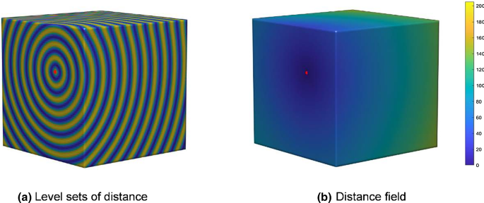

  

  Distance calculation of a certain vertex over the entire surface based on the heat method

  The direction along which the distance increases can be determined and normalised:

  $$ X = - \nabla u/\left| {\nabla u} \right|. $$

  (2)

  Figure 4a demonstrates the level sets of distance from the heat source. The distance fieldφin Fig. 4b is recovered by solving the Poisson equation:

  $$ \Delta \Phi = \nabla \cdot X. $$

  (3)

  For the triangulated surface mesh, Eqs. (1–3) with Laplace operator ($\Delta$), discrete gradient ($\nabla$) and divergence ($\nabla \cdot$) need to be discretised. The discretisation of the Laplacian at the vertex i can be defined as:

  $$ \left( {Lu} \right)_{i} = \left( {2A_{i} } \right)^{ - 1} \mathop \sum \limits_{j} \left( {{\text{cot}}\alpha_{i,j} + cot\beta_{i,j} } \right)\left( {u_{j} - u_{i} } \right) $$

  (4)

  where A_i is one third of the surrounding triangle area incident on vertex i, j are the vertices surrounding vertex i, $\alpha_{i,j}$ and $\beta_{i,j}$ are angles opposing the edge (Fig. 5 a).

  Fig. 5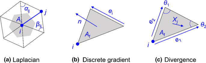

  

  Illustration of triangulated surface mesh processing for the heat method

  Fig. 6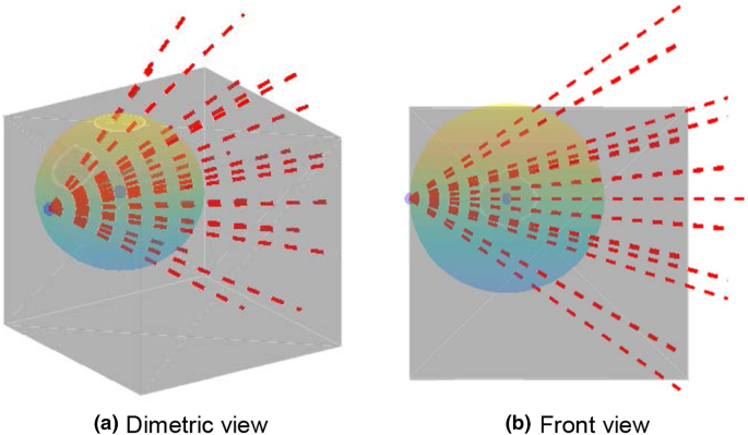

  

  Distance calculation based on the ray shooting method

  The discretisation can also be expressed in matrix form:

  $$ L = A^{ - 1} L_{C} $$

  (5)

  where A contains the vertex area information, and $L_{C}$ is cotan operator.

  The heat flow, u, at time t can be solved using the following equation:

  $$ \left( {A - tL_{C} } \right)u = \delta_{{\Omega }} $$

  (6)

  where $\delta_{{\Omega }}$ is a Kronecker delta over the boundary ${\Omega }$.

  For solving the gradient $\nabla u$, the following discretisation equation is used:

  $$ \nabla u = \left( {2A_{f} } \right)^{ - 1} \mathop \sum \limits_{i} u_{i} \left( {n \times e_{i} } \right) $$

  (7)

  where $A_{f}$ is the triangle surface area, n is the unit normal, and $e_{i}$ is the edge vector oriented counter clockwise (Fig. 5b).

  The discretisation of divergence $\nabla \cdot X$ at the vertex i can be defined as:

  $$ \nabla \cdot X = \frac{1}{2}\mathop \sum \limits_{j} {\text{cot}}\theta_{1} \left( {e_{1} \cdot X_{j} } \right) + {\text{cot}}\theta_{2} \left( {e_{2} \cdot X_{j} } \right) $$

  (8)

  where j are the triangles surrounding vertex i, the $X_{j}$, e₁ and e₂ are the corresponding unit vector and edge vectors (Fig. 5c).

  In the end, the distance field φ can be calculated using the following discretised Poisson equation:

  $$ L_{C} \phi = B $$

  (9)

  where B is the vector of divergences of the normalised vector X.

  For a certain vertex, D1 is defined as the maximum distance in the corresponding distance fieldφ.

• (2) D2 calculation

  A ray shooting method is used to decide a ‘shape aware’ distance inside the geometry (Liu et al., 2009; Shapira et al., 2008). As illustrated in Figure 6, given a certain centroid of a triangle, f_i, a cone is centred around the inward normal direction n_i of this triangle. Twenty (m=20) rays inside the cone are cast into the geometry, and the ray length, l_j, inside the triangle mesh geometry is obtained.

  Fig. 7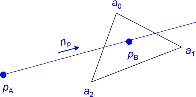

  

  Illustration of ray-triangle intersection

  For calculating the ray length, ray-triangle intersection algorithm developed by Möller et al. (Möller & Trumbore, 1997) is used (Fig. 7). The ray equation R(x) can be defined as:

  $$ R\left( x \right) = p_{A} + x \cdot n_{p} $$

  (10)

  where $p_{A}$ is the ray origin and n_p is the ray direction.

  The implicit equation of the triangle interaction plane is:

  $$ \left( {p - a_{0} } \right) \cdot n = 0 $$

  (11)

  where $a_{0}$ is one vertex of the triangle, n is the normal direction of this triangle (Fig. 7).

  The interaction point position, $p_{B} ,$ can be calculated by combining the above two equations. The length between the ray shooting origin, $p_{A} ,$ and the interaction position, $p_{B} ,$ can be defined as:

  $$ l = \left\| {p_{A} - p_{B} .} \right\| $$

  (12)

  For the centroid in a certain triangle, f_i, the maximal inscribed sphere diameter, d_i, is defined as:

  $$ d_{i} = \arg \min_{j} \left\{ {l_{j} /\cos \theta_{j} } \right\} $$

  (13)

  where θ_j is the angle between l_j and n_j.

  For a certain vertex on the triangulated surface, D2 is defined as an average value of d_i of the neighbourhood triangles. Here, the neighbourhood triangles are defined as triangles sharing the same vertex.

  The AR value of a certain feature depends on the ratio of characteristic length and characteristic width. For evaluating the AR of a certain feature, D1 calculated by heat method represents the characteristic length of a 3D geometry, while D2 calculated by the ray shooting method decides the characteristic width of the geometry. These two measures can be applied to any meshed geometries regardless of their orientations. The dimensionless ratio (D1/D2) could then be used to describe various geometries.

Mesh segmentation algorithm

The above-mentioned dimensionless value D1/D2 offers a way to inspect a meshed geometry on a global level. However, in some cases, the geometry has complex features that need to be isolated and analysed individually. 3D mesh segmentation is one method to achieve this (Theologou et al., 2015). In the presented work, a spectral mesh segmentation method is applied to partition the complex geometries and it is based upon the methods in Liu and Zhang (2004).

The mesh segmentation method starts from a graph representation of the meshed surfaces. A dual graph of the 3D mesh is firstly constructed by connecting the centre node of triangle faces which share common edges (Fig. 8a). Afterwards, a weight matrix, Weight, between adjacent faces f_i and f_j is calculated. Distance measures between adjacent faces are derived on the dual graph and used in the weight matrix. During the segmentation, two faces tend to belong to different parts if they have a large distance value.

Fig. 8

Dual graph, geodesic distance and angular distance for mesh segmentation

Three distance measures i.e. geodesic distance (Geo_Dist), angular distance (Ang_Dist) and volumetric shape image distance (VSI_Dist) are used in this work. As illustrated in Fig. 8b, the geodesic distance (Geo_Dist) is the distance between the centres of adjacent faces:

$$ Geo_{{{\text{Dist}}}} \left( {f_{{\text{i}}} ,f_{{\text{j}}} } \right) = \left\| {p_{{\text{i}}} - p_{{\text{C}}} } \right\| + \left\| {p_{{\text{j}}} - p_{{\text{C}}} } \right\| $$

(14)

where p_i and p_j are the centroids of f_i and f_j, and p_C is the middle point of the common edge.

The angular distance is a criterion to identify concave edges for performing the segmentation. As illustrated in Fig. 8c, the angular distance between two adjacent faces can be defined as:

$$ Ang_{{{\text{Dist}}}} \left( {f_{{\text{i}}} ,f_{{\text{j}}} } \right) = \left\{ {\begin{array}{*{20}c} { acos\left( {n_{i} \cdot n_{j} } \right) if \eta \left( {f_{{\text{i}}} ,f_{{\text{j}}} } \right) > 0 } \\ { \cdot acos\left( {n_{i} \cdot n_{j} } \right) if \eta \left( {f_{{\text{i}}} ,f_{{\text{j}}} } \right) \le 0} \\ \end{array} } \right. $$

(15)

In this work, $\epsilon =0.1$ to emphasise the effect of concave edges.

The convexity $\eta \left( {f_{{\text{i}}} ,f_{{\text{j}}} } \right)$ is calculated by:

$$ \eta \left( {f_{{\text{i}}} ,f_{{\text{j}}} } \right) = \left( {n_{i} \times n_{j} } \right) \cdot n_{e} $$

(16)

where n_i and n_j are normal of f_i and f_j, n_e is the edge vector of the common edge.

The volumetric shape image distance (VSI_Dist) (Katz & Tal, 2003; Liu et al., 2009) is calculated by the previously described ray shooting method. As illustrated in Fig. 9a, the reference point, r_i, of each triangle face, f_i, is defined as the centre of the corresponding inscribed sphere. For each triangle face, f_i, m (m = 100) rays are uniformly sent through a Gaussian sphere, and the interaction point s_i^j between the rays and the meshed surface can be collected (Fig. 9b). The normalised interaction points for a triangle face f_i are:

$$ S_{i} = \left\{ {s_{i}^{1} - r_{i} , \cdots ,s_{i}^{m} - r_{i} } \right\} $$

(17)

Fig. 9

Computation of volumetric shape image (VSI) for mesh segmentation (Modified from Liu et al. (Liu et al., 2009))

This is defined as the volumetric shape image (VSI) for f_i (Fig. 9c).

The difference between two triangle faces f_i and f_j is defined as:

$$ VSI_{{{\text{Dist}}}} \left( {f_{{\text{i}}} ,f_{{\text{j}}} } \right) = \frac{1}{{\mathop \sum \nolimits_{k} w_{k} }}\mathop \sum \limits_{k = 1}^{m/2} w_{k} \left( {l_{i}^{k} - l_{j}^{k} } \right)^{2} $$

(18)

where l^k is the distance difference along the k-th direction:

$$ l^{k} = \left\| {S^{2k - 1} - S^{2k} } \right\| $$

(19)

w_k is the Gaussian distribution:

$$ w_{k} = \left\{ {\begin{array}{*{20}c} {e^{{ - \left( {d_{k} - u_{ave} } \right)^{2} /\left( {2\sigma_{std}^{2} } \right) }} if d_{k} < u_{ave} + 2\sigma_{std} } \\ {0 if d_{k} > u_{ave} + 2\sigma_{std} } \\ \end{array} } \right. $$

(20)

where u_ave is the average value, and σ_std is the standard deviation. d_k is calculated by:

$$ d_{k} = \left( {l_{i}^{k} - l_{j}^{k} } \right)^{2} $$

(21)

The volumetric shape image distance (VSI_Dist) can be used to capture the volumetric feature information.

The pairwise distance matrix, Weight, between adjacent faces is then defined as a combination of the above three distance measures:

$$ Weight\left( {f_{i} ,f_{j} } \right) = \alpha Geo_{Dist} \left( {f_{i} ,f_{j} } \right) + \beta Ang_{Dist} \left( {f_{i} ,f_{j} } \right) + \gamma VSI_{Dist} \left( {f_{i} ,f_{j} } \right) $$

(22)

The parameters α, β and γ are used to control the relative importance of these three distance measures. The pairwise distance, Weight, is subsequently assigned to the constructed dual graph. Afterwards, a distance matrix, Dist, describing the shortest distances between all pairs of faces (f_l and f_m) is calculated. A symmetric normalised affinity matrix, W, can be obtained via a Gaussian kernel function:

$$ W\left( {f_{{\text{l}}} ,f_{{\text{m}}} } \right){ = }e^{{ - Dist\left( {f_{{\text{l}}} , f_{{\text{m}}} } \right)/\left( {2\sigma_{{{\text{ave}}}}^{2} } \right)}} $$

(23)

where σ_ave is defined as the average value of distance matrix Dist. The segmentation based on the k-means clustering method is performed on the selected eigenvectors of the affinity matrix W (Liu & Zhang, 2004), in which the number of segment features N_f needs to be specified.

After this mesh segmentation procedure, the proposed criteria D1/D2 in Sect. 2.1 can be applied to each segmented sub-model.

Results and discussion

Single component

• (1) Evaluation of different geometries using D1/D2

  The proposed dimensionless ratio, D1/D2, is used to describe a group of test geometries, e.g. a thin wall, an ellipsoid and a helix. The prediction results are compared to the known AR values to evaluate performance.

  Figure 10 is a schematic of square shaped geometries: a 100 mm size square (d=100 mm) is extruded to have different lengths (l=0.1–2000 mm). In this way, various types of square shaped geometries can be obtained, e.g. thin wall, cube and rod, corresponding to different ARs. The two distance measures (D1 and D2) are applied for each square shaped geometry. For a certain meshed geometry, D1 and D2 are calculated at each vertex of the surface mesh, thus a set of values can be obtained. Figure 11 illustrates the D1 and D2 distribution for a typical meshed rod geometry. As D1 is calculated based on heat method, the smallest value is distributed in the middle of the geometry while the largest value representing the maximum distance appears at either end of the rod (Fig. 11b). D2 is calculated based on the ray shooting method and has a different distribution characteristic. In particular, the smallest values occur along edge regions of the geometry (Fig. 11c). As illustrated in Fig. 12, probability distributions of these two measures (D1 and D2) are further calculated for several square shaped geometries. The probability distributions are closely related to different shape features: for the thin wall geometry the largest D1 and D2 have the maximum probability, while the cube geometry shows a contrary trend that the smallest value has the maximum probability; the rod geometry has a relatively even probability distribution. The maximum value (D1_max and D2_max) and average value (D1_ave and D2_ave) in the probability graph are then obtained. The corresponding dimensionless ratios (D1_max/D2_max and D1_ave/D2_ave) are further evaluated and compared with the defined AR values as shown in Fig. 13. Here, the AR is defined as the ratio of the longest edge length to the shortest edge length within a geometry. As shown in Fig. 13a, considering different lengths, l, the geometry has different AR values (AR=1–1000). Fig. 13b demonstrates a linear relationship between the D1/D2 and the defined AR in logarithmic scale. The results indicate that D1/D2 can predict the AR of square shaped geometries, which is especially useful for detecting high AR features. It can also be concluded that in most cases D1_max/D2_max has a better prediction accuracy than D1_ave/D2_ave. In the following, only D1_max/D2_max is selected and studied for further evaluation of other geometries.

  The proposed dimensionless D1_max/D2_max is also applied to ellipsoids, as illustrated in Fig. 14. The dimension of an ellipsoid can be described by the length of three principal semi-axes a, b and c, and the AR is defined as the ratio of the longest axis length to the shortest semi-axis length. As shown in this graph, the proposed dimensionless D1_max/D2_max can capture the AR variation trend of the ellipsoids. When the three principal axes have the same length, the geometry becomes a sphere with an aspect ratio value of AR=1. In this case, D1 represents the semi-circumference of a sphere, while D2 is the diameter of a sphere, thus the predicted values are slightly higher than the defined AR. The analysis is performed on various polyhedra with AR=1 (Fig. 15). For all cases, the D1_max/D2_max is slightly larger than the defined aspect ratio (AR=1), which reveals the measure is prone to overestimating the aspect ratio, particularly for the low AR polyhedra. There is also a trend of decreasing D1_max/D2_max with an increasing number of faces from a tetrahedron to sphere. This indicates that this dimensionless measure is sensitive to morphology changes.

  Similar analysis has been performed on curved geometries as illustrated in Figs. 16, 17, and 18. For the curved rod and thin wall geometries (Figs. 16 and 17), they are set to have the same perimeter/thickness and AR values (AR=20 for curved rod, AR=1000 for curved thin wall). For both cases, the degree of curvature changes from 180 to 360 degrees. For the curved rod geometry, the D1_max/D2_max (≈20) can accurately predict the AR when the curved angle is less than 360 degrees. The geometry becomes a closed form when the curved angle is 360 degrees, and the D1_max/D2_max value drops sharply to around 10. For the curved thin wall geometry, the D1_max/D2_max (≈1200) is slightly larger than the defined AR when the curved angle is less than 360 degrees, and is equivalent to the defined AR for the closed form case with a 360 degree curved angle. Similar tendency can also be observed for the helical geometry as shown in Fig. 18. Here, the aspect ratio (AR=31.4) of the helical geometry is defined as the ratio of length (l=157 mm) to diameter (d=5 mm). The D1/D2_max is about 15, which is about half the defined AR (≈31.4) when the height H=0, and it gives a good prediction when H>0. For all cases in Figures 16, 17, and 18, despite the curved geometry, the same characteristics dimensions exist until the geometry becomes fully enclosed. At this point, the D1_max/D2_max values are different to the open-form cases. It can be argued that the topology of the closed-form geometry is fundamentally different to the open-form geometry. Therefore, a precise definition of AR of these geometries needs to be further explored.

• (2) Evaluation of mesh sensitivity

  Triangulated STL files are created with a variety of meshing strategies and levels of refinement. Therefore, it is appropriate to conduct a mesh sensitivity analysis using the proposed criterion D1/D2. As illustrated in Fig. 19, four different mesh numbers (N_mesh) for the cubic geometries have been considered to evaluate the mesh sensitivity. Figure 20 presents the prediction results considering different mesh numbers for typical cubic shaped geometries. In general, for all geometries in Fig. 20, the proposed D1_max/D2_max can give reasonable predictions of aspect ratio values within the examined mesh number range (N_mesh=192–12288). In addition, with increased mesh numbers, the D1_max/D2_max approaches an asymptotic value, and can therefore give more reliable predictions. For the tested geometries used in this work, relatively high mesh numbers (>10000) are adopted to ensure reliable predictions.

Fig. 10

Dimension of square shaped geometries

Fig. 11

D1 and D2 at each vertex within a meshed rod geometry

Fig. 12

Probability distribution of D1 and D2 values within typical square shaped geometries

Fig. 13

Comparison between D1/D2 and theoretically defined aspect ratio (AR) for the square shaped geometries

Fig. 14

Comparison between D1_max/D2_max and theoretically defined aspect ratio (AR) for ellipsoids

Fig. 15

Evaluation of D1_max/D2_max for different polyhedra

Fig. 16

Comparison between D1_max/D2_max and aspect ratio (AR) for the curved rod geometry

Fig. 17

Comparison between D1_max/D2_max and aspect ratio (AR) for the curved thin wall geometry

Fig. 18

Comparison between D1_max/D2_max and aspect ratio (AR) for the helical geometry

Fig. 19

Cubic geometries with different mesh triangle counts

Fig. 20

Mesh sensitivity checks for typical cubic geometries

Geometries with complex features

The developed method was then applied to evaluate geometries with complex features. As illustrated in Fig. 21, D1/D2 at each vertex within each test geometry is firstly calculated. In this figure, high values are usually found for thin wall features (a), sharp edges (c, d and e) and abrupt cross-sectional changes (b) within a component. All of these features are known to be related to complications in metal AM processes. This demonstrates that D1/D2 has the potential to distinguish those problematic features that are closely related to high thermal stresses during AM processes. For evaluating the aspect ratio of individual features within a complex geometry, the mesh segmentation algorithm is applied. As illustrated in Fig. 22, the geometries are segmented using a spectral method and assigned to different colours for different segments. D1_max/D2_max is calculated for each segment and plotted in a bar chart in, where the colour is kept the same as the corresponding segment (see online manuscript for colour information). In this way, high AR features such as the thin walls in Fig. 22a can be distinguished. The results in Figs. 21 and 22 demonstrate the applicability of this method for geometries with complex features.

Fig. 21

D1/D2 distribution at each vertex for different components with complex features

Fig. 22

Mesh segmentation results and corresponding D1_max/D2_max for each segmented part

Discussion and future work

Different test geometries including straightforward and complex features are evaluated using the proposed metrics D1 and D2. These two metrics are generally applicable for triangulated geometries. In addition, D1 and D2 vary at each vertex within a meshed geometry (Fig. 11), thus there is a probability distribution for a certain geometry as illustrated in Fig. 12. In this work, it was found that the maximum value i.e. D1_max and D2_max are most suitable for capturing properties similar to AR for a given geometry. The calculated ratio D1_max/D2_max is a good estimation of the component AR for most cases. Especially, D1_max/D2_max offers a general method to automatically check various high AR features, which will be useful in preventing associated defects during metal AM processing. In addition, the calculated D1/D2 at each vertex shows potential for detecting problematic features such as thin walls and sharp edges (see Fig. 21). The proposed dimensionless ratio is independent of geometry scale and orientations, and can be applicable to all geometrical shapes. It was found that curved geometry with same characteristic length and width, closure of the geometry resulted in a sudden change in the D1_max/D2_max values (Figs. 16, 17, and 18). In this work, the curved geometries shown in Figs. 16, 17, and 18 are assumed to have the same AR values. As the topology of the closed-form geometry and the open-form geometry are fundamentally different, this step change is unsurprising but requires further study to ascertain whether this sudden change is acceptable in the majority of cases.

With regard to geometries with complex features, a mesh segmentation algorithm has been applied to isolate and analyse the individual features (Fig. 22). The spectral method used in this work has shown an impressive capacity to segment distinct features, and the D1_max/D2_max can then be calculated for each individual feature. The proposed method could be used as a general check to distinguish high AR features within complex geometries. It should be noted that the number of segments needs to be defined a priori, which is arguably inconvenient. However, improvements in segmentation algorithms is beyond the scope of the present study (Theologou et al., 2015). An obvious improvement is unsupervised mesh segmentation, which would allow for automatic estimation of segment numbers. More advanced segmentation algorithm could also be applied to this research to analyse geometries that contain a variety of problematic features (Fang et al., 2011; Hase et al., 2020).

The proposed method in this article provides a promising way to automatically detect high AR features of meshed files prior to AM. In general, the developed algorithm can be used to distinguish high AR features for any processes using meshed STL files. There are various kinds of metal AM processes, e.g. powder bed fusion, and wire arc additive manufacturing. As one of the most common AM techniques, the powder bed fusion process could be a main application area of this algorithm, especially as high AR features are one of the major selling points of this process e.g. strut-based lattice structures. Currently, this algorithm is being integrated to a design software for additive manufacturing that can be used as a new manufacturability check for AM components. It will also be useful to combine this algorithm with other computer aided engineering (CAE) tools, especially thermal stress analysis. It can also be used as a criteria to further optimise the geometry design by some other intelligent methods (Jiang et al., 2020; Wang et al., 2020).

As a final discussion point, it is important to note that AR is a property of interest in numerous fields beyond AM. As such, the proposed approach may find useful application in fields such as medical imaging (Lehmann et al., 1999), biological studies (Weir et al., 2003) and, indeed, any other field in which AR is a property of interest.

Conclusions

Detecting problematic features in AM is necessary and has not yet been widely studied. Potential defects in metal AM are often associated with high AR features, e.g. thin walls and fine needle-shaped geometry. In this work, a dimensionless ratio, D1/D2, based on mesh processing algorithms was proposed. This ratio is analogous to the definition of AR (D1 is characteristic length, and D2 is characteristic width). Analysis of various geometries were performed using this method. The main conclusions are as follows:

• 1. Two distance metrics were defined based on heat method (D1) and ray shooting method (D2). The corresponding dimensionless ratios (D1/D2 and D1_max/D2_max) are therefore applied to detect high aspect ratio features of different geometries.

• 2. For most individual components e.g. square shaped geometry, ellipsoids and polyhedra, D1_max/D2_max can successfully predict the AR, especially for the high AR features. The defined dimensionless ratio is useful for characterising a group of similar or related shapes with different AR values.

• 3. If the method is accompanied by mesh segmentation, geometries can be analysed on a feature-by-feature basis, which is a valuable additional functionality. By combining spectral mesh segmentation method, the proposed dimensionless ratio can be used to detect problematic features in a global model.

Currently, there are very few checks that can be readily applied to a general 3D model in order to identify problematic features prior to manufacture. As the complexity of a component increases, it becomes very challenging to isolate problematic regions with confidence. This can be viewed as an important and early step in the avoidance of wasted build-time and material in metal AM. Avoiding these costly failures is paramount if the metal AM process chain (design through to manufacture) is to become productive and reliable in future years. In future, it would be necessary to further testify this algorithm by performing experiments on additive manufactured parts for specific material, machine and process combinations. In addition, it will be useful to combine this method with thermal stress analysis in AM as an integrated design approach.

References

Aspect ratio, https://en.wikipedia.org/wiki/Aspect_ratio.
Bartlett, J. L., & Li, X. (2019). An overview of residual stresses in metal powder bed fusion. Additive Manufacturing, 27, 131–149.
Bhavar, V., Kattire, P., Patil, V., Khot, S., Gujar, K., Singh, R. (2014). A review on powder bed fusion technology of metal additive manufacturing. 4th International conference and exhibition on Additive Manufacturing Technologies-AM-2014. pp. 1–2.
Burns, N., Burns, M., Travis, D., Geekie, L., & Rennie, A. E. (2016). Designing advanced filtration media through metal additive manufacturing. Chemical Engineering & Technology, 39, 535–542.
Campana, G., & Mele, M. (2020). An application to Stereolithography of a feature recognition algorithm for manufacturability evaluation. Journal of Intelligent Manufacturing, 31(1), 199–214.
Compactness measure of a shape, https://en.wikipedia.org/wiki/Compactness_measure_of_a_shape.
Crane, K., Weischedel, C., & Wardetzky, M. (2017). The heat method for distance computation. Communications of the ACM, 60, 90–99.
DebRoy, T., Wei, H., Zuback, J., Mukherjee, T., Elmer, J., Milewski, J., Beese, A. M., Wilson-Heid, A., De, A., & Zhang, W. (2018). Additive manufacturing of metallic components–process, structure and properties. Progress in Materials Science, 92, 112–224.
Demir, A. G. (2018). Micro laser metal wire deposition for additive manufacturing of thin-walled structures. Optics and Lasers in Engineering, 100, 9–17.
Diegel, O., Schutte, J., Ferreira, A., & Chan, Y. L. (2020). Design for additive manufacturing process for a lightweight hydraulic manifold. Additive Manufacturing, 36, 101446.
Fabro, A. T., Meng, H., & Chronopoulos, D. (2020). Uncertainties in the attenuation performance of a multi-frequency metastructure from additive manufacturing. Mechanical Systems and Signal Processing, 138, 106557.
Fang, Y., Sun, M., Kim, M., & Ramani, K. (2011). Heat-mapping: A robust approach toward perceptually consistent mesh segmentation. In CVPR 2011 (pp. 2145-2152). IEEE
Ganeriwala, R., Strantza, M., King, W., Clausen, B., Phan, T. Q., Levine, L. E., Brown, D. W., & Hodge, N. (2019). Evaluation of a thermomechanical model for prediction of residual stress during laser powder bed fusion of Ti-6Al-4V. Additive Manufacturing, 27, 489–502.
Ge, R., Ghadiri, M., Bonakdar, T., & Hapgood, K. (2017). 3D printed agglomerates for granule breakage tests. Powder Technology, 306, 103–112.
Ge, R., Ghadiri, M., Bonakdar, T., Zheng, Q., Zhou, Z., Larson, I., & Hapgood, K. (2020b). Deformation of 3D printed agglomerates: Multiscale experimental tests and DEM simulation. Chemical Engineering Science, 217, 115526.
Ge, R., Humbert, G., Martinez, R., Attallah, M. M., & Sciacovelli, A. (2020a). Additive manufacturing of a topology-optimised multi-tube energy storage device: Experimental tests and numerical analysis. Applied Thermal Engineering, 180, 115878.
Ghasri-Khouzani, M., Peng, H., Rogge, R., Attardo, R., Ostiguy, P., Neidig, J., Billo, R., Hoelzle, D., & Shankar, M. (2017). Experimental measurement of residual stress and distortion in additively manufactured stainless steel components with various dimensions. Materials Science and Engineering: A, 707, 689–700.
Ghouse, S., Babu, S., Van Arkel, R. J., Nai, K., Hooper, P. A., & Jeffers, J. R. (2017). The influence of laser parameters and scanning strategies on the mechanical properties of a stochastic porous material. Materials & Design, 131, 498–508.
Hao, J., Fang, L., Williams, R. E. (2011). An efficient curvature‐based partitioning of large‐scale STL models. Rapid Prototyping Journal
Hase, V. J., Bhalerao, Y. J., Patil, G. V., & Nagarkar, M. P. (2020). Intelligent threshold prediction for hybrid mesh segmentation through artificial neural network. In Computing in Engineering and Technology (pp. 889-899). Springer.
Jiang, J., Xiong, Y., Zhang, Z., & Rosen, D. W. (2020). Machine learning integrated design for additive manufacturing. Journal of Intelligent Manufacturing, 1–14.
Jiang, J., & Ma, Y. (2020). Path planning strategies to optimize accuracy, quality, build time and material use in additive manufacturing: A review. Micromachines, 11, 633.
Jiang, J., Newman, S. T., & Zhong, R. Y. (2021). A review of multiple degrees of freedom for additive manufacturing machines. International Journal of Computer Integrated Manufacturing, 34, 195–211.
Jinoop, A., Paul, C., Mishra, S., & Bindra, K. (2019). Laser Additive Manufacturing using directed energy deposition of Inconel-718 wall structures with tailored characteristics. Vacuum, 166, 270–278.
Katz, S., & Tal, A. (2003). Hierarchical mesh decomposition using fuzzy clustering and cuts. ACM Transactions on Graphics (TOG), 22, 954–961.
Krieger, K. J., Bertollo, N., Dangol, M., Sheridan, J. T., Lowery, M. M., & O’Cearbhaill, E. D. (2019). Simple and customizable method for fabrication of high-aspect ratio microneedle molds using low-cost 3D printing. Microsystems & Nanoengineering, 5, 1–14.
Lehmann, T. M., Gonner, C., & Spitzer, K. (1999). Survey: Interpolation methods in medical image processing. IEEE Transactions on Medical Imaging, 18, 1049–1075.
Levkulich, N., Semiatin, S., Gockel, J., Middendorf, J., DeWald, A., & Klingbeil, N. (2019). The effect of process parameters on residual stress evolution and distortion in the laser powder bed fusion of Ti-6Al-4V. Additive Manufacturing, 28, 475–484.
Liu, R., & Zhang, H. (2004). Segmentation of 3D meshes through spectral clustering. In 12th Pacific Conference on Computer Graphics and Applications, 2004. PG 2004. Proceedings. (pp. 298-305). IEEE.
Liu, R., Zhang, H., Shamir, A., & Cohen‐Or, D. (2009). A part‐aware surface metric for shape analysis. In Computer Graphics Forum (Vol. 28, No. 2, pp. 397-406). Wiley Online Library.
Lu, X., Lin, X., Chiumenti, M., Cervera, M., Hu, Y., Ji, X., Ma, L., Yang, H., & Huang, W. (2019). Residual stress and distortion of rectangular and S-shaped Ti-6Al-4V parts by Directed Energy Deposition: Modelling and experimental calibration. Additive Manufacturing, 26, 166–179.
Luo, Z., & Zhao, Y. (2018). A survey of finite element analysis of temperature and thermal stress fields in powder bed fusion additive manufacturing. Additive Manufacturing, 21, 318–332.
Markl, M., & Körner, C. (2016). Multiscale modeling of powder bed–based additive manufacturing. Annual Review of Materials Research, 46, 93–123.
Xact Metal, Design Guide - Best Practices for Metal Powder-Bed Fusion Additive Manufacturing, https://xactmetal.com/design-guide.pdf.
Möller, T., & Trumbore, B. (1997). Fast, minimum storage ray-triangle intersection. Journal of Graphics Tools, 2, 21–28.
Panesar, A., Abdi, M., Hickman, D., & Ashcroft, I. (2018). Strategies for functionally graded lattice structures derived using topology optimisation for additive manufacturing. Additive Manufacturing, 19, 81–94.
Parry, L., Ashcroft, I., & Wildman, R. D. (2016). Understanding the effect of laser scan strategy on residual stress in selective laser melting through thermo-mechanical simulation. Additive Manufacturing, 12, 1–15.
Parry, L., Ashcroft, I., & Wildman, R. (2019). Geometrical effects on residual stress in selective laser melting. Additive Manufacturing, 25, 166–175.
Pizzolato, A., Sharma, A., Ge, R., Maute, K., Verda, V., & Sciacovelli, A. (2019). Maximization of performance in multi-tube latent heat storage–Optimization of fins topology, effect of materials selection and flow arrangements. Energy, 203, 114797.
Plocher, J., & Panesar, A. (2019). Review on design and structural optimisation in additive manufacturing: Towards next-generation lightweight structures. Materials & Design, 183, 108164.
Robinson, J., Ashton, I., Fox, P., Jones, E., & Sutcliffe, C. (2018). Determination of the effect of scan strategy on residual stress in laser powder bed fusion additive manufacturing. Additive Manufacturing, 23, 13–24.
Schmeiser, F., Krohmer, E., Schell, N., Uhlmann, E., & Reimers, W. (2020). Experimental observation of stress formation during selective laser melting using in situ X-ray diffraction. Additive Manufacturing, 32, 101028.
Shabat, Y. B., & Fischer, A. (2015). Design of porous micro-structures using curvature analysis for additive-manufacturing. Procedia CIRP, 36, 279–284.
Shapira, L., Shamir, A., & Cohen-Or, D. (2008). Consistent mesh partitioning and skeletonisation using the shape diameter function. The Visual Computer, 24, 249.
Simson, T., Emmel, A., Dwars, A., & Böhm, J. (2017). Residual stress measurements on AISI 316L samples manufactured by selective laser melting. Additive Manufacturing, 17, 183–189.
Suard, M., Lhuissier, P., Dendievel, R., Blandin, J.-J., Vignat, F., & Villeneuve, F. (2014). Towards stiffness prediction of cellular structures made by electron beam melting (EBM). Powder Metallurgy, 57, 190–195.
Theologou, P., Pratikakis, I., & Theoharis, T. (2015). A comprehensive overview of methodologies and performance evaluation frameworks in 3D mesh segmentation. Computer Vision and Image Understanding, 135, 49–82.
Thornton, J., Dalay, B., Smith, D. (2016). Additive manufacturing of waveguide for Ku-band satellite communications antenna. In 2016 10th European Conference on Antennas and Propagation (EuCAP), (pp. 1–4). IEEE.
Wang, C., Tan, X. P., Tor, S. B., & Lim, C. S. (2020). Machine learning in additive manufacturing: State-of-the-art and perspectives. Additive Manufacturing, 101538.
Wang, Y., Gao, J., & Kang, Z. (2018). Level set-based topology optimization with overhang constraint: Towards support-free additive manufacturing. Computer Methods in Applied Mechanics and Engineering, 339, 591–614.
Weir, B., Amidei, C., Kongable, G., Findlay, J. M., Kassell, N. F., Kelly, J., Dai, L., & Karrison, T. G. (2003). The aspect ratio (dome/neck) of ruptured and unruptured aneurysms. Journal of Neurosurgery, 99, 447–451.
Wu, A. S., Brown, D. W., Kumar, M., Gallegos, G. F., & King, W. E. (2014). An experimental investigation into additive manufacturing-induced residual stresses in 316L stainless steel. Metallurgical and Materials Transactions A, 45, 6260–6270.
Yoo, D.-J. (2014). Advanced porous scaffold design using multi-void triply periodic minimal surface models with high surface area to volume ratios. International Journal of Precision Engineering and Manufacturing, 15, 1657–1666.
Yu, T., Li, M., Breaux, A., Atri, M., Obeidat, S., & Ma, C. (2019). Experimental and numerical study on residual stress and geometric distortion in powder bed fusion process. Journal of Manufacturing Processes, 46, 214–224.
Funding
Funding was provided by Engineering and Physical Sciences Research Council, Impact Acceleration Account.
Author information
Authors and Affiliations
Corresponding author
Additional information
Publisher's Note
Springer Nature remains neutral with regard to jurisdictional claims in published maps and institutional affiliations.
Rights and permissions
Open Access This article is licensed under a Creative Commons Attribution 4.0 International License, which permits use, sharing, adaptation, distribution and reproduction in any medium or format, as long as you give appropriate credit to the original author(s) and the source, provide a link to the Creative Commons licence, and indicate if changes were made. The images or other third party material in this article are included in the article's Creative Commons licence, unless indicated otherwise in a credit line to the material. If material is not included in the article's Creative Commons licence and your intended use is not permitted by statutory regulation or exceeds the permitted use, you will need to obtain permission directly from the copyright holder. To view a copy of this licence, visit http://creativecommons.org/licenses/by/4.0/.
About this article
Cite this article
Ge, R., Flynn, J. A computational method for detecting aspect ratio and problematic features in additive manufacturing. J Intell Manuf 33, 519–535 (2022). https://doi.org/10.1007/s10845-021-01857-1
Received:
Accepted:
Published:
Issue Date:
DOI: https://doi.org/10.1007/s10845-021-01857-1