Fast state-space methods for inferring dendritic synaptic connectivity

Abstract

We present fast methods for filtering voltage measurements and performing optimal inference of the location and strength of synaptic connections in large dendritic trees. Given noisy, subsampled voltage observations we develop fast l ₁-penalized regression methods for Kalman state-space models of the neuron voltage dynamics. The value of the l ₁-penalty parameter is chosen using cross-validation or, for low signal-to-noise ratio, a Mallows’ C _p -like criterion. Using low-rank approximations, we reduce the inference runtime from cubic to linear in the number of dendritic compartments. We also present an alternative, fully Bayesian approach to the inference problem using a spike-and-slab prior. We illustrate our results with simulations on toy and real neuronal geometries. We consider observation schemes that either scan the dendritic geometry uniformly or measure linear combinations of voltages across several locations with random coefficients. For the latter, we show how to choose the coefficients to offset the correlation between successive measurements imposed by the neuron dynamics. This results in a “compressed sensing” observation scheme, with an important reduction in the number of measurements required to infer the synaptic weights.

Appendices

Appendix A: The quadratic function and the LARS+ algorithm

In this appendix we provide the details of the algorithm used to obtain the solution $\hat W^{ij}(\lambda )$ for all λ, where $i=1\ldots N$ indicates the neuron compartment and $j=1\ldots K$ the presynaptic stimulus associated with the weight. To simplify the notation, define

$$Q(W) \equiv \log p(Y|W),$$

(A.1)

$$Q(W,V) \equiv \log p(Y,V|W),$$

(A.2)

where these expressions are related by

$$p(Y|W) = \int p(Y,V|W)\, dV.$$

(A.3)

Let us first obtain an explicit expression for $Q(W)$. Recall from Section 2 that

$$\begin{array}{@{}rcl@{}} Q(W,V) &=& - \frac12 \sum\limits_{t=1}^{T}{ (y_{t} - B_{t} V_{t})^{T} C_{y}^{-1} (y_{t} - B_{t} V_{t}) }\\ && - \frac12 \sum\limits_{t=2}^{T} { (V_{t} - AV_{t-1} - W U_{t-1})^{T}}\\ &&{\kern2.5pc}\times {C_{V}^{-1} (V_{t} - AV_{t-1} - WU_{t-1}) }\\ && - \frac12 V_{1}^{T} C_{0}^{-1} V_{1} + const.. \end{array}$$

(A.4)

Since $Q(W,V)$ is quadratic and concave in V, we can expand it around its maximum $\hat {V}(W)$ as

$$\begin{array}{@{}rcl@{}} Q(W,V) &=& Q(W,\hat{V}) \\ &&+ \frac12 (V-\hat{V}(W))^{T} H_{VV}(V-\hat{V}(W)), \end{array}$$

(A.5)

where the NT × NT Hessian

$$H_{VV} = \frac{\partial^{2} Q(W,V) }{\partial V \partial V} \,,$$

(A.6)

does not depend on Y or W, as is clear from Eq. A.4. Inserting the expansion (A.5) in the integral Eq. A.3 and taking the log, we get

$$ Q(W) = Q(W,\hat{V}(W))+c$$

(A.7)

$$ = \log p(Y|\hat{V}(W)) + \log p(\hat{V}(W)|W) +c$$

(A.8)

where $c= -\frac 12 \log |-H_{VV}| + \frac {TN}{2}\log 2\pi$ is independent of W.

Since $\hat {V}(W)$ is the maximum of $Q(W,V)$, its value is the solution of $\nabla _{V} Q(W,V)=0$, given by

$$ \hat{V}(W) = -H_{VV}^{-1}Z(W)$$

(A.9)

where

$$Z(W) = \nabla_{V} Q(W,V) |_{V=0} =\left(\begin{array}{c} B_{1}^{T}C_{y}^{-1}y_{1} - A^{T} C_{V}^{-1} WU_{1} \\ B_{2}^{T}C_{y}^{-1}y_{2} - A^{T} C_{V}^{-1} WU_{2} + C_{V}^{-1}WU_{1} \\ B_{3}^{T}C_{y}^{-1}y_{3} - A^{T} C_{V}^{-1} WU_{3} + C_{V}^{-1} WU_{2}\\ \vdots\end{array}\right) \in \mathbb{R}^{NT}, $$

(A.10)

as follows from Eq. A.4. It is useful to expand $Z(W)$ as

$$ Z(W) = Z_{0} + \sum_{i,j}Z_{ij} W^{ij}$$

(A.11)

where the coefficients $Z_{0}, Z_{ij} \in \mathbb {R}^{NT}$ can be read out from Eq. A.10 and are independent of W. This in turn gives an expansion for $\hat {V}$ in Eq. A.9 as

$$ \hat{V}(W) = \hat{V}_{0} + \sum\limits_{i,j}\hat{V}_{ij} W^{ij} \, \,\, \in \, \mathbb{R}^{NT}$$

(A.12)

where

$$ \hat{V}_{0} = -H_{VV}^{-1}Z_{0} \, \,\, \in \, \mathbb{R}^{NT}$$

(A.13)

$$ \hat{V}_{ij} = -H_{VV}^{-1}Z_{ij} \, \,\, \in \, \mathbb{R}^{NT}$$

(A.14)

are independent of W. Note that $\hat {V}_{0}$ has components

$$ \hat{V}_{0} = \left(\begin{array}{lll} (\hat{V}_{0})_{1}\\ {\kern10pt} \vdots \\ (\hat{V}_{0})_{T}\end{array}\right)$$

(A.15)

where each $(\hat {V}_{0})_{t}$ is an N-vector, and similarly for each $\hat {V}_{ij}$.

To obtain the explicit form of $Q(W)$ one can insert the expansion Eq. A.12 for $\hat {V}(W)$ in Eq. A.8. But it is easier to notice first, using the chain rule, that

$$\begin{array}{@{}rcl@{}} \frac{d Q(W,\hat{V}(W)) }{d W} &=& \frac{\partial Q(W,\hat{V}(W))}{\partial W}\\ &&+\frac{\partial Q(W,\hat{V}(W))}{\partial \hat{V}} \frac{\partial \hat{V}(W)}{\partial W} \end{array}$$

(A.16)

$$= \frac{\partial Q(W,\hat{V}(W)) }{\partial W}$$

(A.17)

$$ = C_{V}^{-1} \sum_{t=2}^{T} (\hat{V}_{t} - A\hat{V}_{t-1} - W U_{t-1}) U_{t-1}^{T}$$

(A.18)

where the second term in Eq. A.16 is zero since $\hat {V}(W)$ is the maximum for any W. Thus once $\hat V$ is available, the gradient of Q w.r.t. W is easy to compute, since multiplication by the sparse cable dynamics matrix A is fast. We can now insert Eq. A.12 into the much simpler expression (A.18) to get

$$ \frac{d Q(W,\hat{V}(W)) }{d W^{ij}} = r_{ij} + M_{ij,i^{\prime}j^{\prime}}W^{i^{\prime}j^{\prime}}$$

(A.19)

with $i,i' = 1\ldots N$ and $j,j' = 1 \ldots K$ and coefficients

$$ r_{ij} = \frac{1}{\sigma^{2} dt}\sum\limits^{T}_{t=2}\left((\hat{V}_{0})_{t} - A (\hat{V}_0)_{t-1}\right)_{i} (U_{t-1})_{j}$$

(A.20)

$$\begin{array}{rll} M_{ij,i^{\prime}j^{\prime}} &=&\frac{1}{\sigma^{2} dt}\sum\limits_{t=2}^{T}\left[\left((\hat{V}_{i^{\prime}j^{\prime}})_{t} - A (\hat{V}_{i^{\prime}j^{\prime}})_{t-1}\right)_{i}\right.\\ &&{\kern3.5pc} \left.\times(U_{t-1})_{j} -(U_{t-1})_{j} (U_{t-1})_{j^{\prime}} \delta_{ii^{\prime}} \right]\\ \end{array}$$

(A.21)

where $\delta _{ii^{\prime }}$ is Kronecker’s delta. The desired expression for $Q(W)$ follows by a simple integration of Eq. A.19 and gives the quadratic expression

$$ Q(W) = \sum\limits_{i,j} r_{ij}W^{ij} + \frac12 W^{ij} M_{ij,i^{\prime}j^{\prime}}W^{i^{\prime}j^{\prime}} + const.$$

(A.22)

where $i = 1\ldots N, j = 1\ldots K$. Note that the costly step, computationally, is the linear matrix solve involving H _VV in Eqs. A.13–A.14 to obtain the components of $\hat V$, which are then used in Eqs. A.20–A.21 to obtain $p_{ij}$ and $M_{ij,i'j'}$ in $O(T)$ time. Note that we do not need the explicit form of $H^{-1}_{VV}$, only its action on the vectors $Z_{0}, Z_{ij}$.

Matrix form of coefficients

For just one presynaptic signal (K = 1), we can express the coefficients of the log-likelihood Eq. A.22 in a compact form by defining the matrices

$$ P=\left(\begin{array}{l} -A \quad I_{N}\\ \qquad {\kern3pt} -A I_{N}\\\\\\ \qquad \qquad \qquad \qquad -A I_{N} \\ \qquad \qquad \qquad \qquad \qquad 0 \end{array}\right) \quad \in \mathbb{R}^{NT \times NT}$$

(A.23)

$$ U = (U_{1} I_{N} \quad \cdots \quad U_{T-1}I_{N} 0)\quad \in \mathbb{R}^{N \times NT}$$

(A.24)

$$\begin{array}{@{}rcl@{}} B &=& \begin{pmatrix} B_{1} & \\ & B_{2} & \\ & & . \\ & & &. \\ & & & & B_T \end{pmatrix} \quad \in \mathbb{R}^{ST \times NT} \end{array}$$

(A.25)

and $C^{-1}_{yT} = C^{-1}_{y} I_{ST}$, where $I_{N}$ and $I_{ST}$ are identity matrices of the indicated dimensions. Using these matrices, the expansion (A.12) for the estimated voltages is

$$\hat V(W) = V_{0} + \hat V W$$

(A.26)

with

$$V_{0} = -H_{VV}^{-1} B^{T} C_{yT}^{-1} Y \quad \in \mathbb{R}^{NT}$$

(A.27)

$$\hat V = ( \hat V_{1} \cdots \hat V_{N} )$$

(A.28)

$$ = - H^{-1}_{VV} P^{T} U^{T} C_{V}^{-1} \quad \in \mathbb{R}^{NT \times N} \,.$$

(A.29)

where Y in Eq. A.27 is

$$\begin{array}{@{}rcl@{}} Y =\begin{pmatrix} y_{1} \\ \vdots \\ y_{T} \end{pmatrix} \end{array}$$

(A.30)

The coefficients of the quadratic log-likelihood in Eq. A.22 can now be expressed as

$$r = C_{V}^{-1} U P \hat V_{0}$$

(A.31)

$$= - C_{V}^{-1} U P H_{VV}^{-1} B^{T} C_{yT}^{-1} Y \quad \in \mathbb{R}^{N}$$

(A.32)

and

$$ M = C_{V}^{-1}UP \hat V - ||U||^{2} C_{V}^{-1}$$

(A.33)

$$= - C_{V}^{-1}UP H^{-1}_{VV}P^{T}U^{T}C_{V}^{-1} - ||U||^{2} C_{V}^{-1} \in \mathbb{R}^{N \times N}$$

(A.34)

where we defined $||U||^2= \sum\limits _{t=1}^{T-1} U_{t}^{2}$. Note that this form makes evident that M is symmetric and negative semidefinite, which is not obvious in Eq. A.21. In matrix form, the OLS solution is given by

$$\hat{W} = \arg \max\limits_{W} \, W^{T} r + \frac12 W^TMW$$

(A.35)

$$= -M^{-1}r$$

(A.36)

$$\begin{array}{@{}rcl@{}} &=& - \left( C_{V}^{-1}UU^{T} + C_{V}^{-1}UP H^{-1}_{VV}P^{T}U^{T}C_{V}^{-1} \right)^{-1} \\ &&C_{V}^{-1} U P H_{VV}^{-1} B^{T} C_{yT}^{-1} Y \end{array}$$

(A.37)

$$= - \frac{UP}{||U||^{2}} \left( \frac{P^TU^{T} C_{V}^{-1} UP } {||U||^{2}} + H_{VV} \right)^{-1} B^{T} C_{yT}^{-1} Y ,$$

(A.38)

where in the last line we used the identity

$$(\mathbf A^{-1} \,+\, \mathbf B^{T} \mathbf C^{-1} \mathbf B )^{-1} \mathbf B^{T} \mathbf C^{-1} \,=\, \mathbf A \mathbf B^{T} ( \mathbf B \mathbf A \mathbf B^{T} \,+\, \mathbf C)^{-1} \,.$$

(A.39)

1.1 A.1 LARS-lasso

We will restate here the LARS-lasso algorithm from (Efron et al. 2004) for a generic concave quadratic function $Q(W)$. We are interested in solving²

$$\hat{W}(\lambda) = \arg \max_{\substack{W}} \, L(W,\lambda)$$

(A.40)

where

$$L(W,\lambda) = Q(W) - \lambda \sum_{i=1}^{N} |W^{i}|.$$

(A.41)

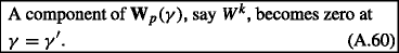
As we saw in Eq. 2.11, the solution for $\hat W$ is a piecewise linear function of λ, with components becoming zero or non-zero at the breakpoints.

As a function of $W^{i}$, $L(W,\lambda )$ is differentiable everywhere except at $W^i=0$. Therefore, if ${W}^{i}$ is non-zero at the maximum of $L(W,\lambda )$, it follows that

$$\frac{d L(W,\lambda)}{d W^{i}} =0 \qquad \text{for} \qquad W^{i} \neq 0\,,$$

(A.42)

or equivalently

$$\nabla_{i} Q(W) \,=\, r_{i} + M_{i,i'}W^{i'} \,=\, \lambda \, sign(W^i)\,\text{for}\, W^{i} \neq 0\,,$$

(A.43)

which implies

$$| \nabla_{i} Q(W)| = \lambda \qquad \text{for} \qquad W^{i} \neq 0\,. $$

(A.44)

For λ = ∞, one can ignore the first term in Eq. A.41, so the solution to Eq. A.40 is clearly $W^{i} =0$. One can show that this holds for all $\lambda > \lambda _{1}$, where

$$\lambda_{1} = \max\limits_{\substack{i}}|\nabla_{i}Q|_{W=0} = \max_{\substack{i}} |r_i|$$

(A.45)

Suppose, without loss of generality, that the maximum in Eq. A.45 occurs for $i=1$. The condition Eq. A.43 will now be satisfied for non-zero $W^{1}$, so we decrease λ and let $W^{1}$ change as

$$\begin{array}{@{}rcl@{}} \lambda &=& \lambda_1-\gamma \\ W^{1}(\gamma) &=& \gamma a^{1} \qquad \qquad \gamma \in [0,\lambda_{1}] \end{array}$$

(A.46)

$$\begin{array}{@{}rcl@{}} \lambda &=& \lambda_1-\gamma \\ W^{1}(\gamma) &=& \gamma a^{1} \qquad \qquad \gamma \in [0,\lambda_{1}] \end{array}$$

(A.47)

while the other $W^{i}$s are kept to zero. To find $a^{1}$, insert Eq. A.47 in Eq. A.43,

$$r_{1} + M_{11} \gamma a^{1} = (\lambda_{1} -\gamma) \, sign(a^1)\,,$$

(A.48)

from which we get $a_1= -{r_{1}}/(\lambda _{1} M_{11}).$ Proceeding in this way, and denoting by $\textbf {W}_{p}(\gamma )$ the vector of weights after the p-th breakpoint, in general we will have, after p steps

$$\lambda = \lambda_p-\gamma$$

(A.49)

$$\textbf{W}_{p}(\gamma) = \textrm{linear\,in} \, \gamma \, \textrm{with} k \leq p \, \textrm{non-zero \, components,}$$

(A.50)

$$| \nabla_{i}Q(\textbf{W}_{p}(\gamma'))| = \lambda_p-\gamma \qquad i=1 \ldots k \;\;\quad \textrm{non-zero directions,}$$

(A.51)

$$| \nabla_{i'}Q(\textbf{W}_{p}(\gamma'))| < \lambda_p-\gamma \qquad i' >k \quad \qquad \;\textrm{zero directions,}$$

(A.52)

and we let γ grow until either of these conditions occurs:

• 1.

If this happens we let $W^{k+1}$ become active. Define

$$\textbf{W}_{p} \equiv \textbf{W}_{p}(\gamma'),$$

(A.54)

$$\lambda_{p+1} = \lambda_{p} - \gamma',$$

(A.55)

and continue with $k+1$ components as:

$$\begin{array}{@{}rcl@{}} \textbf{W}_{p+1}(\gamma)&\equiv& \textbf{W}_{p} + \gamma \textbf{a} \\ &=&{} \begin{pmatrix} W^{1}_{p} \\ \vdots \\ W^{k}_{p} \\ 0 \end{pmatrix}{} +{} \gamma {}\begin{pmatrix} a^{1} \\ \vdots \\ a^{k} \\ a^{k+1} \end{pmatrix}{\kern-1.5pt} \gamma{\kern-1.5pt} \in [0,\lambda_{p+1}] \end{array}$$

(A.56)

$$ \lambda = \lambda_{p+1} - \gamma$$

(A.57)

To find the new velocity a, insert $\textbf {W}_{p+1}(\gamma )$ into Eq. A.43 to get

$$\begin{array}{@{}rcl@{}} \begin{pmatrix} M_{11} \ldots M_{1(k+1)} \\ \vdots\\ \vdots\\ M_{(k+1)1} \ldots M_{(k+1)(k+1)} \end{pmatrix} \begin{pmatrix} a^{1} \\ \vdots \\ a^{k} \\ a^{k+1} \end{pmatrix} = - \begin{pmatrix} sign(W^{1}_p)\\ \vdots\\ sign(W^{k}_p) \\ sign(a^{k+1}) \end{pmatrix}\\ \end{array}$$

(A.58)

In this equation we need $sign(a^{k+1})$, which, as we show in Section A.3, coincides with that of the derivative computed in Eq. A.53,

$$\begin{array}{@{}rcl@{}} sign(a^{k+1}) = sign(\nabla_{k+1}Q(\textbf{W}_{p}(\gamma')))\,. \end{array}$$

(A.59)

• 2.

If this happens, $W^{k}$ must drop from the active set because the path of $\textbf {W}_{p}(\gamma )$ was obtained assuming a definite sign for $W^{k}$ in Eq. A.43. So we define

$$\textbf{W}_{p} = \textbf{W}_{p}(\gamma'),$$

(A.61)

$$\lambda_{p+1} = \lambda_{p} - \gamma',$$

(A.62)

drop $W^{k}$ from the active set and continue with $k-1$ active components as:

$$\begin{array}{@{}rcl@{}} \textbf{W}_{p+1}(\gamma) &\equiv& \textbf{W}_{p} + \gamma \textbf{a} = \begin{pmatrix} W^{1}_{p} \\ \vdots \\ W^{k-1}_{p} \end{pmatrix} \\ &&+ \gamma \begin{pmatrix} a^{1} \\ \vdots \\ a^{k-1} \end{pmatrix} \qquad\gamma \in [0,\lambda_{p+1}]\end{array}$$

(A.63)

$$ \lambda = \lambda_{p+1} - \gamma$$

(A.64)

To find the new a, inserting $\textbf {W}_{p+1}(\gamma )$ into Eq. A.43 gives

$$\begin{array}{@{}rcl@{}} \begin{pmatrix} M_{11} \ldots M_{1(k-1)}\\ \vdots\\ M_{(k-1) 1} \ldots M_{(k-1)(k-1)} \end{pmatrix} \begin{pmatrix} a^{1} \\ \vdots \\ a^{k-1}\end{pmatrix} = - \begin{pmatrix} sign(W^{1}_p)\\ \vdots \\ sign(W^{k-1}_p)\end{pmatrix}\\ \end{array}$$

(A.65)

from which a can be solved.

As each a is found, we decrease λ by increasing $\gamma$, and check again for either cases 1 or 2 until we reach λ = 0, at which point all directions will be active and the weights will correspond to the global maximum of Q(W).

Having presented the algorithm, let us discuss its computational cost. To obtain $p_{i}$ we need to act with $H_{VV}^{-1}$ on $Z_{0}$ (see Eqs. A.13 and A.20). Similarly, for each new active weight $W^{k+1}$ the $(k+1)$-th column of M is needed in Eq. A.58, which comes from acting with $H_{VV}^{-1}$ on $Z_{k+1}$ (see Eqs. A.14 and A.21). The action of $H_{VV}^{-1}$ has a runtime of O(TN ³), but in Appendix C we show how to reduce it to $O(TNS^2)$ with a low-rank approximation. For the total computational cost, we have to add the runtime of solving Eq. A.58. Since at each breakpoint the matrix in the left-hand side of Eq. A.58 only changes by the addition of the $(k+1)$th row and column, the solution takes $O(k^2)$ instead of $O(k^3)$ (Efron et al. 2004). Running the LARS algorithm through k steps, the total cost is then $O(kTNS^{2} + k^3)$ time.

1.2 A.2 Enforcing a sign for the inferred weights

We can enforce a definite sign for the non-zero weights by a simple modification of the LARS-lasso. Assuming for concreteness an excitatory synapse, the solution to Eq. A.40 for all λ and subject to

$$W^{i} \geq 0$$

can be obtained by allowing a weight to become active only if its value along the new direction is positive. The enforcement of this condition for the linear regression case was discussed in Efron et al. (2004). In our formulation of the LARS-lasso algorithm, the positivity can be enforced by requiring that the first weight becomes active when

$$\lambda_{1} = \max\limits_{\substack{i}} r_{i} \qquad r_{i} >0 $$

(A.66)

and by replacing the condition that triggers the introduction of new active weights, denoted above as condition 1, by

• 1.

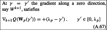
By requiring the derivative along $W^{k+1}$ to be positive at the moment of joining the active set, we guarantee that $W^{k+1}$ will be positive due to the result of Section A.3.

When λ reaches zero, the weights, some of which may be zero, are the solution to the quadratic program

$$\begin{array}{@{}rcl@{}} \hat{W} = \arg \max\limits_{\substack{W}} \, Q(W) \,, \qquad W^{i} \geq 0\,. \end{array}$$

(A.68)

We will refer to the LARS-lasso algorithm with the modification Eq. A.67 as LARS+. In practice, the measurements can be so noisy that the algorithm may have to be run assuming both non-negative and non-positive weights, and the nature of the synapse can be established by comparing the likelihood of both results at their respective maxima. More generally, if $K>1$ we have to estimate the sign of each presynaptic neuron; this can be done by computing the likelihoods for each of the $2^{K}$ possible sign configurations. This exhaustive approach is tractable since we are focusing here on the small-K setting; for larger values of K, approximate greedy approaches may be necessary (Mishchenko et al. 2011).

1.3 A.3 The sign of a new active variable

Property the sign of a new variable $W^{k+1}$ which joins the active group is the sign of $\nabla _{k+1} Q(W)$ at the moment of joining.

Proof

Remember that the matrix $M_{ii'}$ is negative definite and, in particular, its diagonal elements are negative

$$M_{ii} < 0\,, \qquad i = 1 \ldots N $$

(A.69)

As we saw in Section A.1, if the first variable to become active is

$$\textbf{W}_{1}(\gamma) = \gamma a^{1} \qquad \qquad \gamma \in [0,\lambda_{1}] $$

(A.70)

with

$$\lambda_{1} = \max_{\substack{i}}|\nabla_{i}Q|_{W=0} = |r_1| \,, $$

(A.71)

we have

$$a_1= -\frac{r_{1}}{\lambda_{1} M_{11}} $$

(A.72)

and using Eq. A.69 and $\lambda _{1} >0$ we get

$$sgn(a_1) = sgn(r_1) $$

(A.73)

as claimed. Suppose now that there are k active coordinates and our solution is

$$\begin{array}{@{}rcl@{}} \mathbf{W}_{p}(\gamma) = \left(\right. \begin{array}{l} W^{1}_{p}(\gamma)\\ \cdot \\ \cdot \\ W^{k}_{p}(\gamma)\end{array} \left.\right) \gamma \in [0,\lambda_{p}] \end{array}$$

(A.74)

Define

$$c_{j}(\gamma) = \nabla_{j}Q({\bf{W}}_{p}(\gamma))\,, $$

(A.75)

and note that

$$|c_{j}(\gamma)| = \lambda_{p} - \gamma \qquad j = 1 \ldots k \,. $$

(A.76)

Suppose a new variable $W^{k+1}$ enters the active set at $\gamma =\gamma '$ such that

$$|c_{k+1}(\gamma')| = \lambda_{p} - \gamma' $$

(A.77)

It is easy to see that when taking $\gamma$ all the way to $\lambda _{p}$, the sign of $c_{k+1}(\gamma )$ does not change

$$sgn(c_{k+1}(\gamma')) = sgn(c_{k+1}(\lambda_{p})) $$

(A.78)

since the $c_{j}(\gamma )$ ($j=1, \ldots k$) go faster towards zero than $c_{k+1}(\gamma )$. To make the variable $W^{k+1}$ active, define

$$\lambda_{p+1} = \lambda_{p} - \gamma' \,,$$

(A.79)

$$ \textbf{W}_{p} \equiv \textbf{W}_{p}(\gamma') \,,$$

(A.80)

and continue with $k+1$ components as:

$$\begin{array}{rll}\textbf{W}_{p+1}(\gamma) &\equiv& \textbf{W}_{p} + \gamma \textbf{a} = \left(\begin{array}{l} W^{1}_{p} \\ \vdots\\ W^{k}_{p} \\ 0 \end{array} \right)\\ &&+ \gamma\left(\begin{array}{l} a^{1} \\ \vdots \\ a^{k} \\ a^{k+1} \end{array}\right)\qquad \gamma \in [0,\lambda_{p+1}]\end{array}$$

(A.81)

$$\lambda = \lambda_{p+1} - \gamma$$

(A.82)

To find a, impose on Eq. A.81 the conditions (A.43) that give

$$\textbf{p} + \textbf{M}_{(k+1,k+1)}{\bf{W}_{p+1}}(\gamma) = (\lambda_{p+1} - \gamma) \textbf{s} $$

(A.83)

where $\textbf {p} = (p_{1} , \ldots , p_{k+1})^{T}$, $\textbf {M}_{(k+1,k+1)}$ is the $(k+1) \times (k+1)$ submatrix of $M_{ij}$, and

$$\begin{array}{@{}rcl@{}} \mathbf{s} = \left(\begin{array}{l} sgn(W^{1}_p) \\ . \\ . \\ sgn(W^{k}_{p}) \\ sgn(a^{k+1}) \end{array} \right) \end{array}$$

(A.84)

Since Eq. A.83 holds for any $\gamma$, we get the two equations

$$\begin{array}{@{}rcl@{}} \mathbf{p} + \mathbf{M}_{(k+1,k)}\textbf{W}_{p} = \lambda_{p+1} \textbf{s} \end{array}$$

(A.85)

and

$$\begin{array}{@{}rcl@{}} \textbf{M}_{(k+1,k+1)} {\bf{a}} = -\textbf{s}. \end{array}$$

(A.86)

where $\textbf {M}_{(k+1,k)}$ is obtained from $\textbf {M}_{(k+1,k+1)}$ by eliminating the last column. Inserting Eq. A.85 into Eq. A.86 we get

$$\mathbf{a} = - \frac{1}{\lambda_{p+1}}\mathbf{M}^{-1}_{(k+1, k+1)}(\mathbf{p} + \mathbf{M}_{(k+1, k)} \mathbf{W}_{p})$$

(A.87)

$$\begin{array}{@{}rcl@{}}= - \frac{1}{\lambda_{p+1}} \textbf{M}^{-1}_{(k+1, k+1)} \left(\textbf{p} + \textbf{M}_{(k+1,k)}\textbf{W}_{p}(\lambda_{p}) \right.\\ && \left. - \textbf{M}_{(k+1, k)}\textbf{W}_{p}(\lambda_{p})+ \textbf{M}_{(k+1,k)}\textbf{W}_{p}\right) = - \frac{1}{\lambda_{p+1}} \textbf{M}^{-1}_{(k+1, k+1)}\left(\begin{array}{l} \mathbf{0} \\ c_{k+1}(\lambda_{p}) \end{array}\right) \end{array}$$

(A.88)

$$- \frac{1}{\lambda_{p+1}} (\mathbf{W}_p-\textbf{W}_{p}(\lambda_{p}))$$

(A.89)

where 0 has k elements. Since the $(k+1)$-th element of the second term in Eq. A.89 is zero, we get

$$\begin{array}{@{}rcl@{}} a^{k+1} = - \frac{\left(\textbf{M}^{-1}_{(k+1, k+1)} \right)_{(k+1)(k+1)}}{\lambda_{p+1}} \, c_{k+1}(\lambda_{p}). \end{array}$$

(A.89)

Since $\textbf {M}^{-1}_{(k+1, k+1)}$ is negative definite, we have $\left(\textbf {M}^{-1}_{(k+1, k+1)} \right )_{(k+1)(k+1)} <0$, so using Eq. A.78, the result

$$sgn(a^{k+1}) = sgn(c_{k+1}(\gamma'))$$

(A.91)

follows. □

Appendix B: The C _p criterion for low SNR

In the limit of very low signal-to-noise ratio, we can ignore the dynamic noise term in Eq. 2.1 and consider

$$\begin{array}{@{}rcl@{}} V_{t+dt} &=& A V_{t} + W U_{t} \\ y_{t} &=& B_{t} V_{t} + \eta_{t}, \qquad \qquad \qquad \eta_{t} \sim \mathcal{N}(0, C_{y}I). \end{array}$$

(B.1)

$$\begin{array}{@{}rcl@{}} V_{t+dt} &=& A V_{t} + W U_{t} \\ y_{t} &=& B_{t} V_{t} + \eta_{t}, \qquad \qquad \qquad \eta_{t} \sim \mathcal{N}(0, C_{y}I). \end{array}$$

(B.2)

Let us assume that the number of presynaptic neurons is K = 1 to simplify the formulas. The results can be easily extended to the general case. We can combine the above equations as

$$Y = X W + \eta,$$

(B.3)

where we defined

$$Y = \left(\begin{array}{l} y_{1} \\ \vdots \\ y_{T} \end{array}\right) \qquad \qquad \eta = \left(\begin{array}{l} \eta_{1} \\ \vdots \\ \eta_{T} \end{array}\right)$$

(B.4)

and the matrix X is given by the product

$$X = B C \qquad \in \mathbb{R}^{ST \times N} \,,$$

(B.5)

where B was defined in Eq. A.25 and

$$C = \left(\begin{array}{l}0\\ U_{1} \\ AU_{1} + U_{2} \\ A^2U_{1} + AU_{2} + U_{3} \\ . \\ . \\ A^{T-2}U_{1} + \cdots + U_{T-1} \end{array}\right)\qquad \in \mathbb{R}^{NT \times N} \,.$$

(B.6)

Equation (B.3) corresponds to a standard linear regression problem and the l ₁-penalized posterior log-likelihood to maximize is now

$$\log p(W|Y, \lambda) = - \frac12 ||Y- X W ||^{2} - \lambda \sum_{i=1}^{N} |W^{i}| \,.$$

(B.7)

The solution $\hat W(\lambda )$ that maximizes Eq. B.7 is obtained, as in the general case, using the LARS/LARS+ algorithm, and the fitted observations are given by

$$\hat Y(\lambda) = BC \hat W(\lambda) \,.$$

(B.8)

One can show that each row in $C \hat W(\lambda )$ corresponds to the $C_{V} \rightarrow 0$ limit of the expected voltage $\hat V_{t}(\lambda )$ defined in Eq. 2.11. Given an experiment $(Y,U)$, consider the training error

$$\text{err}(\lambda) = || Y -\hat Y(\lambda)||^2$$

(B.9)

and the in-sample error

$$\text{Err}_{\text in}(\lambda) = \mathbb{E}_{\tilde Y} [ || \tilde Y -\hat Y(\lambda)||^{2} ].$$

(B.10)

In $\text {Err}_{\text in}(\lambda )$, we compute the expectation over new observations $\tilde Y$ for the same stimuli $U_{t}$ and compare them to the predictions $\hat Y(\lambda )$ obtained with the initial experiment $(Y,U)$. Thus, $\text {Err}_{\text in}(\lambda )$ gives a measure of the generalization error of our results. $\text {Err}_{\text in}(\lambda )$ itself cannot be computed directly, but we can compute its expectation with respect to the original observations Y. For this, let us consider first the difference between $\text {Err}_{\text in}$ and err, called the optimism (Friedman et al. 2008). Denoting the components of Y with an index i, it is easy to verify that the expected optimism with respect to Y is

$$\omega(\lambda) \equiv \langle \text{Err}_{\text in}(\lambda) - \text{err}(\lambda) \rangle$$

(B.11)

$$= 2 \sum\limits_{i=1}^{ST} \langle Y_{i} \hat Y_{i}(\lambda) \rangle - \langle Y_{i} \rangle \langle \hat Y_{i}(\lambda) \rangle$$

(B.12)

$$= 2 \sum\limits_{i=1}^{ST} \text{Cov}(Y_{i}, \hat Y_{i}(\lambda)) \,.$$

(B.13)

For the general case $K \geq 1$, we will have $X \in \mathbb {R}^{ST \times NK}$. Let us assume that ST > NK and that X is full rank, that is, rank$(X) = NK$. Then in Zou et al. (2007) it was shown that if we define $d(\lambda )= || \hat W(\lambda )||_{0}$ as the number of non-zero components in $\hat W(\lambda )$, we have⁴

$$\omega(\lambda) = 2 \langle d(\lambda) \rangle \, C_y.$$

(B.14)

Thus $2 d(\lambda ) \, C_{y}$ is an unbiased estimate of $\omega (\lambda )$, and is also consistent (Zou et al. 2007). With this result, and using err$(\lambda )$ as an estimate of $\langle \text {err}(\lambda ) \rangle$, we obtain an estimate of the average generalization error $\langle \text {Err}_{\text in}(\lambda ) \rangle$ as

$$ C_{p}(\lambda) = || Y -\hat Y(\lambda)||^{2} + 2 d(\lambda) \, C_y.$$

(B.15)

This quantity can be used to select the best λ as that value that minimizes $C_{p}(\lambda )$. Since the first term is a non-decreasing function of λ (Zou et al. 2007), it is enough to evaluate $C_{p}(\lambda )$ for each d at the smallest value of λ at which there are d active weights in $W(\lambda )$. With a slight abuse of notation, the resulting set of discrete values of Eq. B.15 will be denoted as C _p (d).

Appendix C: The low-rank block-Thomas algorithm

In this appendix we will present a fast approximation technique to perform multiplications by the inverse Hessian $H_{VV}^{-1}$. The NT × NT Hessian H _VV in Eq. A.6 takes the block-tridiagonal form

$$\begin{array}{lll}H_{VV} &=& \begin{pmatrix}-C_0^{-1} - A^T A & A^T & \mathbf{0} & \mathellipsis \\A & - I - A^T A & A^T & \mathbf{0} & \mathellipsis \\\mathbf{0} & A & - I - A^T A & A^T & \mathbf{0} \\\vdots & \vdots & \vdots & \ddots \\ & \hdots & & A & -I \\\end{pmatrix}\\&&- \begin{pmatrix} B_1^T C_y^{-1}B_1 \\ & B_2^T C_y^{-1}B_2 \\ & & \\ & & B_T^T C_y^{-1}B_T \\\end{pmatrix}\end{array}$$

(C.1)

where we have set $C_{V} = I$ to simplify the notation. We will restore it below to a generic value.

It will be convenient, following (Paninski 2010), to adopt for $C_{0}$, the covariance of the initial voltage $V_{1}$, the value

$$C_{0} = \sum\limits_{i=0}^{\infty}(AA^T)^{i} = (I-AA^T)^{-1}$$

(C.2)

(note that the dynamics matrix A is stable here, ensuring the convergence of this infinite sum). This is the stationary prior covariance of the voltages V _t in the absence of observations y _t , and with this value for $C_{0}$, the top left entry in the first matrix in Eq. C.1 simplifies to $-C_{0}^{-1}-A^TA = -I$.

We want to calculate

$$H_{VV}^{-1}\mathbf{b} = H_{VV}^{-1}\left( \begin{array}{l} b_{1} \\ b_{2} \\ \vdots \\ b_{T} \end{array}\right) = \left(\begin{array}{l} x_{1} \\ x_{2} \\ \vdots \\ x_{T} \end{array} \right)= \mathbf{x},$$

(C.3)

where $\mathbf {b}$ can be an arbitrary NT-dimensional vector and each $b_{i}$ and $x_{i}$ is a column vector with length N. We can calculate this using the block Thomas algorithm for tridiagonal systems of equations (Press et al. 1992), which in general requires $O(N^3T)$ time and $O(N^2T)$ space, as shown in Algorithm 1.

We can adapt this algorithm to yield an approximate solution to Eq. C.3 in $O(TNS^2)$ time by using low-rank perturbation techniques similar to those used in Paninski (2010), Huggins and Paninski (2012), and Pnevmatikakis et al. (2012b). The first task is to calculate $\alpha _{1}^{-1}$. Using the Woodbury matrix lemma, we get

$$\alpha_{1}^{-1} = -(I + B_{1}^{T} C_{y}^{-1}B_1)^{-1}$$

(C.4)

$$= - I + B_{1}^{T} (C_{y} + B_1B_{1}^T)^{-1} B_{1} $$

(C.5)

$$= - I + L_{1} D_{1} L_{1}^{T} \quad \in \mathbb{R}^{N \times N}$$

(C.6)

where

$$L_{1} = B_{1}^{T} \quad \in \mathbb{R}^{N \times S}$$

(C.7)

and

$$\begin{array}{@{}rcl@{}} D_{1} = (C_{y} + B_{1} B_{1}^T)^{-1} \quad \in \mathbb{R}^{S \times S} . \end{array}$$

(C.8)

Note that the simple expression (C.6) for $\alpha _{1}^{-1}$ follows from the form we chose in Eq. C.2 for $C_{0}$. Plugging $\alpha _{1}^{-1}$ into the Algorithm 1’s expression for $\gamma _{1}$ gives

$$\gamma_{1} = \alpha_{1}^{-1} A^{T}$$

(C.9)

$$= - A^{T} + L_{1} D_{1} L_{1}^{T} A^{T} \quad \in \mathbb{R}^{N \times N}.$$

(C.10)

To continue the recursion for the other $\alpha _{i}^{-1}$s, the idea is to approximate these matrices as low-rank perturbations to $-I$,

$$\begin{array}{@{}rcl@{}} \alpha_{i}^{-1} \approx -I + L_{i} D_{i} L_{i}^{T} \quad \in \mathbb{R}^{N \times N} \,, \end{array}$$

(C.11)

where $D_{i}$ is a small $d_{i} \times d_{i}$ matrix with $d_{i} \ll N$ and $L_{i} \in \mathbb {R}^{N \times d_{i}}$. This in turn leads to a form similar to Eq. C.10 for $\gamma _{i}$,

$$\gamma_{i} \approx -A^{T} + L_{i} D_{i} L_{i}^{T} A^T.$$

(C.12)

Therefore we can write

$$\alpha_{i}^{-1} = -(I + A^{T} A + B_{i}^{T} C_{y}^{-1}B_{i} + A \gamma_{i-1})^{-1}$$

(C.13)

$$\begin{array}{@{}rcl@{}}\approx -\left(I + A^{T} A + B_{i}^{T} C_{y}^{-1}B_{i} \right.\\ &&\left.- AA^{T} + A L_{i-1} D_{i-1} L_{i-1}^{T} A^{T} \right)^{-1} \end{array}$$

(C.14)

$$\approx \,-\,(I \,+\, B_{i}^{T} C_{y}^{-1}B_{i} \,+\, A L_{i-1} D_{i-1} L_{i-1}^{T} A^{T} )^{-1}{} .$$

(C.15)

This expression justifies our approximation of $\alpha _{i}^{-1}$s as a low rank perturbation to $-I$: the term $B_{i}^{T} C_{y}^{-1}B_{i}$ is low rank because the number of measurements is $S \ll N$, and the second term is low rank because the condition $eigs(A)<1$ tends to suppress at step i the contribution of the previous step encoded in $L_{i-1} D_{i-1} L_{i-1}^{T}$. See Pnevmatikakis et al. (2012b) for details.

To apply Woodbury we choose a basis for the two non-identity matrices,

$$O_{i} = [A L_{i-1} \quad B_{i}^{T}] \in \mathbb{R}^{N \times (S+d_{i-1})}$$

(C.16)

and write

$$B_{i}^{T} C_{y}^{-1}B_{i} + A L_{i-1} D_{i-1} L_{i-1}^{T} A^{T} = O_{i} M_{i} O_{i}^{T},$$

(C.17)

where

$$M_{i} =\begin{array}{ll} D_{i-1} & \\ & C_{y}^{-1}\end{array} \in \mathbb{R}^{(S + d_{i-1}) \times (S+d_{i-1})}$$

Applying Woodbury gives

$$\alpha_{i}^{-1} = -(I + O_{i} M_{i} O_{i}^T)^{-1}$$

(C.18)

$$= - I + O_{i}(M_{i}^{-1} + O_{i}^{T} O_i)^{-1}O_{i}^T.$$

(C.19)

We obtain $L_{i}$ and $D_{i}$ by truncating the SVD of the expression on the right-hand side: in Matlab, for example, do

$$\begin{array}{@{}rcl@{}} [L',D'] = svd(O_{i}(M_{i}^{-1} + O_{i}^{T} O_i)^{-1/2},\text{`econ' }), \end{array}$$

(C.20)

then choose $L_{i}$ as the first $d_{i}$ columns of $L'$ and $D_{i}$ as the square of the first $d_{i}$ diagonal elements $D'$, where $d_{i}$ is chosen to be large enough (for accuracy) and small enough (for computational tractability).

We must handle $\alpha _{T}^{-1}$ slightly differently because of the boundary condition. Making use of the fact that $C_{0}^{-1} = I - AA^{T}$ and the Woodbury identity, we get

$$\alpha_{T}^{-1} = -\left(I + B_{T}^{T} C_{y}^{-1}B_{T} + A \gamma_{T-1}\right)^{-1}$$

(C.21)

$$\begin{array}{@{}rcl@{}} & = & -\left(I + B_{T}^{T} C_{y}^{-1}B_{T} - AA^{T} \right. \\ &&\left.\qquad+ A L_{T-1} D_{T-1} L_{T-1}^{T} A^{T} \right)^{-1}\end{array}$$

(C.22)

$$= -\left(C_{0}^{-1} + O_{T} M_{T} O_{T}^{T} \right)^{-1}$$

(C.23)

$$ = -C_{0} + C_{0} O_{T} \left(M_{T}^{-1} + O^{T}_{T} C_{0} O_{T}\right)^{-1} O_{T}^{T} C_{0} $$

(C.24)

$$= -C_{0} + L_{T} D_{T} L_{T}^{T},$$

(C.25)

where

$$L_{T} = C_{0} O_T$$

(c.26)

and

$$D_{T} = \left(M_{T}^{-1} + O_{T}^{T} C_{0} O_{T}\right)^{-1}.$$

(C.27)

Multiplications by $\alpha _{T}^{-1}$ are efficient since we can multiply by $C_{0}$ in $O(N)$ time, expoiting the sparse structure of A (see Paninski (2010) for details). It is unnecessary to control the rank because we will only be performing one multiplication with $\alpha _{T}^{-1}$ and calculating the SVD is a relatively expensive operation.

The updates for calculating $y_{i}$ and $x_{i}$ are straightforward:

$$y_{1} = \alpha_{1}^{-1} b_{1}$$

(C.28)

$$= - b_{1} + L_{1} D_{1} L_{1}^{T} b_{1} $$

(C.29)

$$y_{i} = \alpha_{i}^{-1}\left(b_{i} - C_{V}^{-1}Ay_{i-1}\right) $$

(C.30)

$$= \left(-I + L_{i} D_{i} L_{i}^{T}\right)(b_{i} - Ay_{i-1})$$

(C.31)

$$ x_{T} = \alpha_{T}^{-1}\left(b_{T} - C_{V}^{-1}Ay_{T-1}\right) $$

(C.32)

$$ = \left(-C_{0} + L_{T} D_{T} L_{T}^{T}\right)(b_{T} - Ay_{T-1})$$

(C.33)

$$x_{i}= y_{i} - \gamma_{i} x_{i+1}$$

(C.34)

$$= y_{i} + A^{T} x_{i+1} - L_{i} D_{i} L_{i}^{T} A^{T} x_{i+1}.$$

(C.35)

Algorithm 2 summarizes the full procedure. One can verify that the total computational cost scales like $O(TNS^2)$ (see Pnevmatikakis et al. (2012b) for details).

Finally, note that for repeated calls to $H^{-1}_{VV}\mathbf {b}$, we can compute the matrices $L_{i},D_{i}$ once and store them. For the case when $C_{V}$ is not the identity we can apply a linear whitening change of variables $V'_{t} = C_{V}^{-1/2} V_{t}$. We solve as above except we make the substitution $B_{t} \to B_{t} C_{V}^{1/2}$ and our final solution now has the form

$$\mathbf{x} = \left( I_{T} \otimes C_{V}^{1/2} \right) H_{VV}^{-1} \left( I_{T} \otimes C_{V}^{1/2} \right)^{T} \mathbf{b}.$$

References

Barbour, B., Brunel, N., Hakim, V., Nadal, J.-P. (2007). What can we learn from synaptic weight distributions? TRENDS in Neurosciences, 30(12), 622–629.
Bloomfield, S., & Miller, R. (1986). A functional organization of ON and OFF pathways in the rabbit retina. Journal of Neuroscience, 6(1), 1–13.
Candes, E., Romberg, J., Tao, T. (2006). Stable signal recovery from incomplete and inaccurate measurements. Communications on Pure and Applied Mathematics, 59(8), 1207–1223.
Candès, E., & Wakin, M. (2008). An introduction to compressive sampling. IEEE Signal Processing Magazine, 25(2), 21–30.
Canepari, M., Djurisic, M., Zecevic, D. (2007). Dendritic signals from rat hippocampal CA1 pyramidal neurons during coincident pre- and post-synaptic activity: a combined voltage- and calcium-imaging study. Journal of Physiology, 580(2), 463–484.
Canepari, M., Vogt, K., Zecevic, D. (2008). Combining voltage and calcium imaging from neuronal dendrites. Cellular and Molecular Neurobiology, 28, 1079–1093.
Djurisic, M., Antic, S., Chen, W.R., Zecevic, D. (2004). Voltage imaging from dendrites of mitral cells: EPSP attenuation and spike trigger zones. Journal of Neuroscience, 24(30), 6703–6714.
Djurisic, M., Popovic, M., Carnevale, N., Zecevic, D. (2008). Functional structure of the mitral cell dendritic tuft in the rat olfactory bulb. Journal of Neuroscience, 28(15), 4057–4068.
Dombeck, D.A., Blanchard-Desce, M., Webb, W.W. (2004). Optical recording of action potentials with second-harmonic generation microscopy. Journal of Neuroscience, 24(4), 999–1003.
Durbin, J., Koopman, S., Atkinson, A. (2001). Time series analysis by state space methods (Vol. 15). Oxford: Oxford University Press.
Efron, B. (2004). The estimation of prediction error. Journal of the American Statistical Association, 99(467), 619–632.
Efron, B., Hastie, T., Johnstone, I., Tibshirani, R. (2004). Least angle regression. Annals of Statistics, 32, 407–499.
Fisher, J.A.N., Barchi, J.R., Welle, C.G., Kim, G.-H., Kosterin, P., Obaid, A.L., Yodh, A.G., Contreras, D., Salzberg, B.M. (2008). Two-photon excitation of potentiometric probes enables optical recording of action potentials from mammalian nerve terminals in situ. Journal of Neurophysiology, 99(3), 1545–1553.
Friedman, J., Hastie, T., Höfling, H., Tibshirani, R. (2007). Pathwise coordinate optimization. The Annals of Applied Statistics, 1(2), 302–332.
Friedman, J., Hastie, T., Tibshirani, R. (2008). The elements of statistical learning. Springer.
Gelman, A., Carlin, J., Stern, H., Rubin, D. (2004). Bayesian data analysis. CRC press.
Geman, S., Bienenstock, E., Doursat, R. (1992). Neural networks and the bias/variance dilemma. Neural Computation, 4(1), 1–58.
Gobel, W., & Helmchen, F. (2007). New angles on neuronal dendrites in vivo. Journal of Neurophysiology, 98(6), 3770–3779.
Hines, M. (1984). Efficient computation of branched nerve equations. International Journal of Bio-Medical Computing, 15(1), 69–76.
Huber, P. (1964). Robust estimation of a location parameter. The Annals of Mathematical Statistics, 35(1), 73–101.
Huggins, J., & Paninski, L. (2012). Optimal experimental design for sampling voltage on dendritic trees. Journal of Computational Neuroscience (in press).
Huys, Q., Ahrens, M., Paninski, L. (2006). Efficient estimation of detailed single-neuron models. Journal of Neurophysiology, 96, 872–890.
Huys, Q., & Paninski, L. (2009). Model-based smoothing of, and parameter estimation from, noisy biophysical recordings. PLOS Computational Biology, 5, e1000379.
Iyer, V., Hoogland, T.M., Saggau, P. (2006). Fast functional imaging of single neurons using random-access multiphoton (RAMP) microscopy. Journal of Neurophysiology, 95(1), 535–545.
Knopfel, T., Diez-Garcia, J., Akemann, W. (2006). Optical probing of neuronal circuit dynamics: genetically encoded versus classical fluorescent sensors. Trends in Neurosciences, 29, 160–166.
Kralj, J., Douglass, A., Hochbaum, D., Maclaurin, D., Cohen, A. (2011). Optical recording of action potentials in mammalian neurons using a microbial rhodopsin. Nature Methods.
Larkum, M.E., Watanabe, S., Lasser-Ross, N., Rhodes, P., Ross, W.N. (2008). Dendritic properties of turtle pyramidal neurons. Journal of Neurophysiology, 99(2), 683–694.
Lin, Y., & Zhang, H. (2006). Component selection and smoothing in multivariate nonparametric regression. The Annals of Statistics, 34(5), 2272–2297.
Mallows, C. (1973). Some comments on Cp. Technometrics, pp. 661–675.
Milojkovic, B.A., Zhou, W.-L., Antic, S.D. (2007). Voltage and calcium transients in basal dendrites of the rat prefrontal cortex. Journal of Physiology, 585(2), 447–468.
Mishchenko, Y., & Paninski, L. (2012). A Bayesian compressed-sensing approach for reconstructing neural connectivity from subsampled anatomical data. Under review.
Mishchenko, Y., Vogelstein, J., Paninski, L. (2011). A Bayesian approach for inferring neuronal connectivity from calcium fluorescent imaging data. Annals of Applied Statistics, 5, 1229–1261.
Mitchell, T.J., & Beauchamp, J.J. (1988). Bayesian variable selection in linear regression. Journal of the American Statistical Association, 83(404), 1023–1032.
Nikolenko, V., Watson, B., Araya, R., Woodruff, A., Peterka, D., Yuste, R. (2008). SLM microscopy: Scanless two-photon imaging and photostimulation using spatial light modulators. Frontiers in Neural Circuits, 2, 5.
Nuriya, M., Jiang, J., Nemet, B., Eisenthal, K., Yuste, R. (2006). Imaging membrane potential in dendritic spines. PNAS, 103, 786–790.
Pakman, A., & Paninski, L. (2013). Exact hamiltonian Monte Carlo for truncated multivariate gaussians. Journal of Computational and Graphical Statistics, preprint arXiv:1208.4118.
Paninski, L. (2010). Fast Kalman filtering on quasilinear dendritic trees. Journal of Computational Neuroscience, 28, 211–28.
Paninski, L., & Ferreira, D. (2008). State-space methods for inferring synaptic inputs and weights. COSYNE.
Paninski, L., Vidne, M., DePasquale, B., Ferreira, D. (2012). Inferring synaptic inputs given a noisy voltage trace via sequential Monte Carlo methods. Journal of Computational Neuroscience (in press).
Peterka, D., Takahashi, H., Yuste, R. (2011). Imaging voltage in neurons. Neuron, 69(1), 9–21.
Pnevmatikakis, E.A., & Paninski, L. (2012). Fast interior-point inference in high-dimensional sparse, penalized state-space models. Proceedings of the 15th International Conference on Artificial Intelligence and Statistics (AISTATS) 2012, La Palma, Canary Islands. Volume XX of JMLR: W&CP XX.
Pnevmatikakis, E.A., Kelleher, K., Chen, R., Saggau, P., Josić, K., Paninski, L. (2012a). Fast spatiotemporal smoothing of calcium measurements in dendritic trees, submitted. PLoS Computational Biology, 8, e1002569.
Pnevmatikakis, E.A., Paninski, L., Rad, K.R., Huggins, J. (2012b). Fast Kalman filtering and forward-backward smoothing via a low-rank perturbative approach. Journal of Computational and Graphical Statistics (in press).
Press, W., Teukolsky, S., Vetterling, W., Flannery, B. (1992). Numerical recipes in C. Cambridge: Cambridge University Press.
Reddy, G.D., & Saggau, P. (2005). Fast three-dimensional laser scanning scheme using acousto-optic deflectors. Journal of Biomedical Optics, 10(6), 064038.
Sacconi, L., Dombeck, D.A., Webb, W.W. (2006). Overcoming photodamage in second-harmonic generation microscopy: Real-time optical recording of neuronal action potentials. Proceedings of the National Academy of Sciences, 103(9), 3124–3129.
Sjostrom, P.J., Rancz, E.A., Roth, A., Hausser, M. (2008). Dendritic excitability and synaptic plasticity. Physiological Reviews, 88(2), 769–840.
Smith, C. (2013). Low-rank graphical models and Bayesian analysis of neural data: PhD Thesis, Columbia University.
Song, S., Sjöström, P.J., Reigl, M., Nelson, S., Chklovskii, D.B. (2005). Highly nonrandom features of synaptic connectivity in local cortical circuits. PLoS Biology, 3(3), e68.
Studer, V., Bobin, J., Chahid, M., Mousavi, H., Candes, E., Dahan, M. (2012). Compressive fluorescence microscopy for biological and hyperspectral imaging. Proceedings of the National Academy of Sciences, 109(26), E1679–E1687.
Takahashi, N., Kitamura, K., Matsuo, N., Mayford, M., Kano, M., Matsuki, N., Ikegaya, Y. (2012). Locally synchronized synaptic inputs. Science, 335(6066), 353–356.
Tibshirani, R. (1996). Regression shrinkage and selection via the lasso. Journal of the Royal Statistical Society. Series B, 58, 267–288.
Vucinic, D., & Sejnowski, T.J. (2007). A compact multiphoton 3d imaging system for recording fast neuronal activity. PLoS ONE, 2(8), e699.
Yuan, M., & Lin, Y. (2006). Model selection and estimation in regression with grouped variables. Journal of the Royal Statistical Society: Series B (Statistical Methodology), 68(1), 49–67.
Zou, H., & Hastie, T. (2005). Regularization and variable selection via the elastic net. Journal of the Royal Statistical Society: Series B (Statistical Methodology), 67(2), 301–320.
Zou, H., Hastie, T., Tibshirani, R. (2007). On the degrees of freedom of the lasso. The Annals of Statistics, 35(5), 2173–2192.
Acknowledgments
This work was supported by an NSF CAREER grant, a McKnight Scholar award, and by NSF grant IIS-0904353. This material is based upon work supported by, or in part by, the U. S. Army Research Laboratory and the U. S. Army Research Office under contract number W911NF-12-1-0594. JHH was partially supported by the Columbia College Rabi Scholars Program. AP was partially supported by the Swartz Foundation. The computer simulations were done in the Hotfoot HPC Cluster of Columbia University. We thank E. Pnevmatikakis for helpful discussions and comments.
Conflict of interests
The authors declare that they have no conflict of interest.
Author information
Authors and Affiliations
Corresponding author
Additional information
Action Editor: Misha Tsodyks