
Abstract
This paper presents a detailed verification of the Gale-Shapley algorithm for stable matching (or marriage). The verification proceeds by stepwise transformation of programs and proofs. The initial steps are on the level of imperative programs, ending in a linear time algorithm. An executable functional program is obtained in a last step. The emphasis is on the stepwise development of the algorithm and the required invariants.
1 Introduction
The Gale-Shapley algorithm [8] solves a matching problem: it finds a stable matching between two sets of elements given an ordering of preferences for each element. This work spawned a subfield of research, stable matching. The algorithm is of great practical importance: variations of it have been used for matching medical school students and hospital training programs since the 1950s [11] and are used today for matching clients and servers in Akamai’s content delivery network [20]. The textbook by Kleinberg and Tardos [14] presents the problem and the algorithm as the first of five representative algorithm design problems. Shapley and Roth were awarded the 2012 Prize in Economic Sciences in Memory of Alfred Nobel “for the theory of stable allocations”. Nevertheless, no formally verified correctness proof of the algorithm can be found in the literature (see Sect. 14).
This paper presents the first formally verified development of a linear-time executable implementation of the Gale-Shapley algorithm (using the proof assistant Isabelle [24, 25]). The formalization is available online [23]. The development of the final algorithm is by stepwise transformation. By accident we discovered a small defect in a proof rule in a well-known program verification textbook [2, 3] that had gone unnoticed for 30 years (see Sect. 9).
2 Problem and Algorithm
We start with the informal presentation of the problem and algorithm by Gusfield and Irving in their well-known monograph [11]. However, our terminology avoids all reference to gender.Footnote 1
There are two disjoint sets A and B with n elements each. Each element has a strictly ordered preference list of all the members of the other set. Element p prefers q to \(q'\) iff q precedes \(q'\) on p’s preference list. The problem is to find a stable matching, i.e. a subset of A \(\times \)B, with the following properties:
-
Every \(a \in \) A is matched with exactly one \(b \in \) B and vice versa.
-
The matching is stable: there are no two elements from opposite sets who would rather be matched with each other than to the elements they are actually matched with.
The Gale-Shapley algorithm (Algorithm 0) is guaranteed to find such a stable matching in \(O(n^2)\) iterations. Moreover, because the \(a \in \) A get to choose, the resulting matching is A-optimal: there is no other stable matching between A and B with the given preferences where some \(a \in \) A does better, i.e. is matched to a \(b \in \) B that a prefers to the computed match.

3 Isabelle Notation
Isabelle types are built from type variables, e.g.
 , and (postfix) type constructors, e.g.
 . The infix function type arrow is
 . The notation
\(t \,{::}\, \tau \) means that term t has type
\(\tau \). Isabelle (more precisely Isabelle/HOL, the logic we work in) provides types
. The notation
\(t \,{::}\, \tau \) means that term t has type
\(\tau \). Isabelle (more precisely Isabelle/HOL, the logic we work in) provides types
 and
and
 of sets and lists of elements of type
 . They come with the following notations:
 (the image of set
 under
under
 ), function
 (conversion from lists to sets),
 (list with head
 and tail
 ),
),
 (length of list
 ),
),
 (the
(the
 th element of
 starting at 0), and
 (list
(list
 where the
 th element has been replaced by
 ). Throughout the paper, all numbers are of type
 , the type of natural numbers.
Data type
 is also predefined:

4 Hoare Logic and Stepwise Development
Most of the work in this paper is carried out on the level of imperative programs. The Hoare logic used for this purpose is based on work by Gordon [10] and was added to Isabelle by Nipkow in 1998. Possibly the first published usage was by Mehta and Nipkow [21]. Recently Guttmann and Nipkow added variants, i.e. expressions of type
 that should decrease with every iteration of a loop. Total correctness Hoare triples have the syntax
 where
where
 and
and
 are pre- and post-conditions and
 is the program. Loops must be annotated with invariants and variants like this:

The implementation of the Hoare logic comes with a verification condition generator.
We progress from the first to the last algorithm by stepwise transformation. In each step we restate the full modified algorithm, which is not an issue for algorithms of 15–20 lines. Readjusting the proofs to a modified algorithm is reasonably easy: the proofs of the verification conditions are all relatively short (about 60 lines per algorithm), they are structured and readable [26, 27], and our transformation steps are small. Most importantly, the key steps in the proofs are formulated as separate lemmas that are reused multiple times. For example, we may have an algorithm with some set variable
 , prove some lemma about
 , refine the algorithm by replacing
 by a list variable
 , and reuse the very same lemma with
 instantiated by
 .
.
Although this methodology is inspired by stepwise refinement, in particular data refinement, we avoid the word refinement because it suggests a modular development. Instead we speak of stepwise transformation or development and of data concretisation.
This methodology is not intended for the development of large algorithms but for small intricate ones. I can confidently say that it worked well for Gale-Shapley: I spent most of my time on the core proofs and very little on copy-paste-modify. Structured proofs helped to localize the effect of most changes. The problems of code duplication in programming do not arise because the theorem prover keeps you honest.
It should be mentioned that there is a refinement framework in Isabelle [18] and it would be interesting to see how the development of Gale-Shapley plays out in it.
5 Formalization of the Stable Matching Problem
We do not refer to the actual sets A and B and their elements directly but only to their indices
\(0,\dots ,n-1\). We use mnemonic names like
 and
and
 to indicate which of the two sets these indices range over. We speak of
 ’s and
 ’s to mean sets of indices. By
 we abbreviate the set of all
 .
.
We fix the following variables:
-
The cardinality

-
The preference lists
 ,
,
 . For each
 ,
,
 is the preference list of
 , i.e. a list of all b’s in decreasing order of preference. Dually for
 . We assume that the preference lists have the right lengths and are permutations of
 :
:
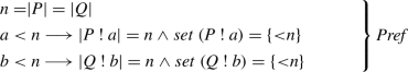
These properties are used implicitly in proofs we discuss.

 ,
,
 . For each
 ,
,
 is the preference list of
 , i.e. a list of all b’s in decreasing order of preference. Dually for
 . We assume that the preference lists have the right lengths and are permutations of
 :
:

It is important to emphasize that although we model everything in terms of lists, in a last step these lists will be implemented as arrays to obtain constant time access to each element.
The notation
 means that
 occurs before
 (meaning
 is preferred to
 ) in the preference list
 :
:

The algorithm tries to match each
 first with
 , then with
 etc. Thus we do not record
 ’s current match
 but we record the
 , and increment
 every time a match
 has to be undone. A list

 (of length
 ) will record the index for the current match of each
 . The actual match
 is
is
 and we define

Note that unless the algorithm has really matched
 and
and
 , then
 is merely the current top choice of
 .
.
In the sequel,
 will always represent such a list of indices into the preference lists. The predicate
 expresses that
 associates every
 with some
 :
:

This means that
 is a function from
 to
to
 .
.
To improve readability we introduce the following suggestive notation:

where
 .
.
5.1 Stable Matchings
We are looking at the special case of bipartite matching where every
 and
and
 are connected. A matching on
 is an injective function from M to
 .
.

The predicate
 means that
 is injective on
 .
.
We want a stable matching, i.e. one where there are no “unstable” matches
 and
and
 such that
 prefers b’ to
 and b’ prefers
 to a’:

We will not just show that the Gale-Shapley algorithm finds a stable matching but also that this matching is A-optimal, i.e. there is no stable matching where some
 can do better:

The dual property is B-pessimality, i.e. no
 can do worse:

Unsurprisingly, it is easy to prove that any A-optimal
 is
is
 -pessimal:

5.2 Stepwise Development
The following points remain unchanged throughout the development process:
-
The matchings are recorded as a variable
 as described above. How it is recorded if some
 has been matched to
 or not changes during the development process.
 -
The precondition always assumes
 , where
 is a list of

 ’s. That is, all
 ’s start at the beginning of their preference list. Making this assumption a precondition avoids a trivial initialization loop. We will frequently deal with initializations like this.
 -
The postcondition is always

 as described above. How it is recorded if some
 has been matched to
 or not changes during the development process.
 , where
 is a list of

 ’s. That is, all
 ’s start at the beginning of their preference list. Making this assumption a precondition avoids a trivial initialization loop. We will frequently deal with initializations like this.
6 Algorithm 1
Algorithm 1 follows the informal algorithm by Gusfield and Irving [11] quite closely. Variable
 records the set of
 ’s that have been matched. Initially no
 has been matched.

At the beginning of each iteration an unmatched
 is picked via Hilbert’s choice operator:
 is some
 that satisfies
 . If there is no such
 , we cannot deduce anything (nontrivial) about
 . However, we only use the choice operator in cases where there is a suitable
 . If there are multiple
 ,
,
 will return an arbitrary fixed one. Although the choice is deterministic, our proofs work by merely assuming that some suitable
 has been picked and thus the algorithm would work just as well with a nondeterministic choice. In the end, the exact nature of
 is irrelevant: only the first two programs use
 , it is transformed away afterwards.
The term (
 ) expresses the inverse of
 applied to
 .
.
In each iteration, one of three possible basic actions is performed, where
 is unmatched and
 :
:
-
match (line 5):
 was unmatched; now
 is matched (to
 ).
). -
swap (line 8):
 was matched to some
 but
but
 prefers
 to
to
 ; now
; now
 is unmatched and moves to the next element on its preference list and
 is matched (to
 )
) -
next (line 9):
 was matched to some
 and
and
 prefers
 to
to
 ; now
; now
 moves to the next element on its preference list.
 was unmatched; now
 is matched (to
 ).
). was matched to some
 but
but
 prefers
 to
to
 ; now
; now
 is unmatched and moves to the next element on its preference list and
 is matched (to
 )
) was matched to some
 and
and
 prefers
 to
to
 ; now
; now
 moves to the next element on its preference list.
We will now detail the correctness proof, first of the invariant, then of the variant.
6.1 The Invariant

The predicate
 says that if
 prefers
 to its match
 then
then
 is matched to some a’ who
 prefers to
 . This is the invariant way of expressing this more operational or temporal property used by Knuth [16] (adapted):

An alternative formulation of
 is based directly on the indices below
 :
:

where
 is the prefix version of the infix !. Both predicates are equivalent

and we use whichever is more convenient in a given situation.
The invariant can be seen as a generalization of the postcondition. The missing link is this lemma from which it follows directly that the invariant together with
 implies the postcondition:
Lemma 1

Proof
By contradiction. Assume there are
 ,
,
 ,
,
 such that
 and
and
 . Assumption
 implies that there is an
 such that
 and
and
 . Injectivity of
 on
on
 implies
 and thus we have both
 and
and
 , a contradiction.
\(\square \)
, a contradiction.
\(\square \)
The precondition
 is easily seen to establish the invariant.
6.2 Preservation of the Invariant
We need to show that
 is preserved by the basic actions match, swap and next. For match this is easy and we concentrate on swap and next. We present the proofs bottom up, starting with the key supporting lemmas.
We begin by showing that
 is preserved. Both swap and next increment some
 where
where
 and
and
 (swap:
 instead of
 ). We need to show that the result is still
 . This is the corresponding lemma:
Lemma 2

Proof
By contradiction. If
 , then
 (by assumptions). Moreover
 because
 . Thus
 and hence
 . This is a contradiction because
 implies
 .
\(\square \)
.
\(\square \)
The following lemma (proof omitted) shows that
 is preserved by swap and next:
Lemma 3

The following three lemmas (of which the first one is straightforward) express that
 is preserved by the three basic actions match, swap and next.
Lemma 4

Lemma 5

Proof
Preservation of
 follows from Lemma 2, preservation of injectivity is straightforward and preservation of
 follows from Lemma 3. It remains to prove
 where
where
 and
and
 :
:

where we have already replaced
 by
by
 because
 implies
 . Now we distinguish if
 or not.
If
 then
then
 and we have to show

If
 ,
,
 yields a witness
 . It remains to show that there is also a witness
 . This follows in the critical case
 because
 does the job:
 and
and
 imply
imply
 because
 .
.
If
 then
then

 . If
. If
 the claim follows from
 . The fact that any witness
 is also in
 follows because
 would imply
 , a contradiction. If
 then
then
 is a suitable witness.
\(\square \)
is a suitable witness.
\(\square \)
Lemma 6

The proof is similar to the one of the preceding lemma, but simpler.
6.3 The Variants
Our variants (see Sect. 4) are of the form
 where
where
 counts the number of iterations and
 is some upper bound. It will follow trivially from our definitions of
 that it increases with every iteration. Thus
 decreases if the invariant and the loop condition imply
 ; the latter is required because subtraction on
 stops at 0.
The term
 is clearly an upper bound of the number of iterations. If the loop body executes in constant time, we can conclude that the loop has complexity
 .
.
6.3.1 A Simple Variant
Examining the loop body of Algorithm 1 we see that with each iteration either
 increases (action match) or it stays the same and one
 (where
 ) increases (actions swap and next). Thus
 is
is
 . Because
 is bounded by
 and we will prove that every
 (where
 ) is bounded by
 , there is an obvious upper bound of
 . A possible variant is given by the following function of
 and
and
 :
:

The following easy properties show that
 is decreased by all three basic actions:

This is the variant that Hamid and Castleberry [13] work with, except that they do not have
 but increment A ! a where we add
 to
to
 . However, we can do better.
6.3.2 The Precise Variant
Knuth [16] improves the
 bound to
 based on this exercise:

Gusfield and Irving [11] argue that this bound follows because “the algorithm terminates when the last
 is matched for the first time”. We will now give a formal proof that is more in line with Knuth’s text and does not require the temporal “first” and “last”.
Knuth’s exercise amounts to the following proposition: there is at most one unmatched
 that is down to its last preference.
Corollary 1

This is a corollary to the following lemma: if an unmatched
 has arrived at the end of its preference list, then all other
 ’s are matched.
Lemma 7

Proof
From
 it follows that
 and thus
 is injective on
 and thus in particular on
 (because
 ). Hence
 (1). Assumption
 implies
 (2). From
 and
and
 it follows that
 (3). Combining (1), (2) and (3) yields
 and thus
 .
\(\square \)
.
\(\square \)
Now we can prove the key upper bound for
 :
:
Lemma 8

Proof
From Lemma 2 we have
 . We distinguish two cases. If there is an
 such that
 and
and
 then, because there is at most one such
 (by Corollary 1), it follows that
 and thus


 . If there is no such
 , then
 and thus


 .
\(\square \)
.
\(\square \)
The assumptions of Lemma 8 imply
 and hence

Thus the following definition of var makes sense:

The following easy properties (except that one has to be careful about subtraction) show that
 is decreased by all three basic actions. The invariant together with
 implies the assumptions of Lemma 8 which imply

7 Algorithm 2
Algorithm 2 is the result of a data concretisation step: the set
 of matched
 ’s is replaced by a list
 of unmatched
 ’s. Thus the abstraction function
 from lists to sets is

 . (Note that formally it is only an abstraction function if the
 -choice is nondeterministic.) The program treats the list
 like a stack: functions
 and
and
 return the head and the tail of the stack. In addition to the invariant
 we also need the well-formedness of
 :
:

Thus the complete invariant is
 .
.

To exemplify our stepwise development approach we consider preservation of the invariant
 by the basic action match (line 6) where
 abbreviates
 . That is, we assume
 ,
,
 ,
,
 and
and
 . Thus
 for some
 ,
,
 and
and
 (using
 ). Now Lemma 4 applies and we conclude
 which implies
 , which is what we actually need to show. In summary, the translation between the two state spaces requires some bridging properties, but then we can apply the abstract lemmas.
From now on, we do not present correctness lemmas or proofs anymore but only annotated programs because the annotations are the key. Of course we still present all variants, invariants and non-trivial auxiliary definitions.
8 Algorithm 3
This data concretisation step addresses the issue that the algorithm needs to find out if the prospective match of some
 is already matched and to whom. Algorithm 3 records the inverse of
 as a variable


 . Eventually
 will be implemented by arrays. We call a function

 a map. Maps come with an update notation:


Function
 inverts
 :
:
 . The notation
 denotes the list
 .
.
The new variable
 requires its own invariant:

where
 . In a nutshell,
 is the inverse of
 . Preservation of
 by all three basic actions is a one-liner.
9 Algorithm 4
In this step we eliminate the list
 . The resulting algorithm is (more or less) the one that Knuth [16] analyzes. The main idea: with each basic action, either the top of
 changes or it is popped. Thus we don’t need to record all of
 but only how far we have popped it. The new variable
 does just that. It starts with
 and is incremented after each match step. This can also be viewed as a data concretisation:
 and
and
 represent
 .
.
Instead of one we now have two loops. In the inner loop, swap and match actions are performed, followed by a single match action. That is,
 is initialized with
 and the inner loop tries to find an unmatched
 for
for
 , possibly unmatching some
 in the process.

The invariants
 and
and
 are unchanged, and the set
 of matched
 ’s is simply
 . In the inner loop,
 because we are looking for a match for
 .
.
The outer variant is
 . Note that the syntax permits us to remember that value of the outer variant in an auxiliary variable, here
 . The point is that we need to show that the outer variant is not incremented by the inner loop. Hence we remember its value in
 and add the invariant
 . Although Isabelle’s Hoare logic formalization goes back more than 20 years, it was only recently extended with variants for total correctness (by Walter Guttmann). In the process of verifying the Gale-Shapely algorithm Nipkow noticed that invariants need to refer to variants and generalized Guttmann’s extension. He also noticed that the account in the textbook by De Boer et al. [2] (which has not changed from the “first edition” [3]) is incomplete, which the authors confirmed (private communication). Their definition of valid proof outlines (programs annotated with (in)variants) [2, Definition 3.8] does not allow inner invariants to refer to outer variants: replacing
\(S^{**}\) by S in the side condition for z fixes the problem.
. Although Isabelle’s Hoare logic formalization goes back more than 20 years, it was only recently extended with variants for total correctness (by Walter Guttmann). In the process of verifying the Gale-Shapely algorithm Nipkow noticed that invariants need to refer to variants and generalized Guttmann’s extension. He also noticed that the account in the textbook by De Boer et al. [2] (which has not changed from the “first edition” [3]) is incomplete, which the authors confirmed (private communication). Their definition of valid proof outlines (programs annotated with (in)variants) [2, Definition 3.8] does not allow inner invariants to refer to outer variants: replacing
\(S^{**}\) by S in the side condition for z fixes the problem.
Finally we consider the inner variant:

To show that
 decreases when
 (or
(or
 ) are incremented we consider one loop iteration with initial value
 and final value
 . Note that because the invariant again holds for
 , Lemma 8 implies that
 .
.

The initial value of
 is
is
 . Because the outer loop does not modify
 ,
,
 is an upper bound on the total number of iterations of the inner loop, i.e. the number of swap and next actions. To this we must add the exactly
 match actions of the outer loop to arrive at an upper bound of
 actions, just like before.
10 Algorithm 5
In this step we implement

 by two lists (think arrays):
 records which
 ’s have been matched with some
 and
and


 says which
 . This is expressed by the following abstraction function:


At this point it is helpful to introduce names for the two invariants:

11 Algorithm 6
In this step we implement the inefficient test
 . Instead of finding the index of
 and
and
 in the list
 we replace
 by a list of lists that map
 ’s to their index, i.e. their rank in the preference lists. From
 we construct the new data structure
 as
as
 where
where

If the list update operation is constant-time (which it will be with arrays),
 is a linear-time algorithm and thus
 can be computed in time
 . A more intuitive but less efficient definition of
 is
is

The two definitions coincide if
 .
.
In Algorithm 6, the only operations used are arithmetic, list indexing
 and pointwise list update
 . If we implement the latter with constant-time operations on arrays (as we will, in the next section), each assignment and each test takes constant time. Thus the overall execution time of the algorithm is proportional to the number of executed tests and assignments. Clearly the outer loop, without the inner one, takes time O(n). As analyzed in the previous section, the inner loop body is executed at most
 times. Thus the overall complexity of the algorithm is
\(O(n) + O(n^2) = O(n^2)\). Because the input,
times. Thus the overall complexity of the algorithm is
\(O(n) + O(n^2) = O(n^2)\). Because the input,
 and
and
 , is also of size
 we have a linear-time algorithm.

12 Algorithm 7
In a final step (on the imperative level) we implement lists by arrays. The basis is Lammich’s and Lochbihler’s Collections library [17, 19] that offers imperative implementations of arrays with a purely functional, list-like interface specification. The basic idea is due to Baker [4, 5] and guarantees constant time access to arrays provided they are used in a linear manner (i.e. no access to old versions), which our arrays obviously are, because the programming language is imperative.
Algorithm 7 is not displayed because it is Algorithm 6 with
 replaced by
 ,
,
 replaced by "array_set xs i x" and
 replaced by
 , where
 (below:
 ),
),
 (below:
 ) and
) and
 (below:
 ) are defined in the Collections library. Correctness of this data concretisation step is proved via the abstraction function
 and refinement lemmas like
 .
.
This is our final imperative algorithm. It has linear complexity, as explained in the previous section. Although the programming language has a semantics that can in principle be executed, Isabelle provides no support for that. Therefore we now recast the last imperative algorithm as recursive functions in Isabelle’s logic, which can be executed in Isabelle [1] or exported to standard functional languages [12].
13 Algorithm 8, Functional Implementation

We translate the imperative code directly into two functions
 and
and
 (Algorithm 8) using the combinator

from the Isabelle library [22]. It comes with the recursion equation

for execution and a Hoare-like proof rule (not shown) for total correctness involving a wellfounded relation on the state space. With its help and the lemmas used in the proof of Algorithm 7 we can show the main correctness theorem:
 computes a stable matching that is A-optimal:

where
 converts
 from lists to arrays and
 converts
 into
into
 in array-form, i.e.
 behaves like
 , but on arrays. Both
 ,
,
 (which are straightforward and not shown) are linear-time functions. Thus the conversion from lists to arrays does not influence the time and space complexity of the algorithm. The complexity is still
 because all basic operations are constant-time and the wellfounded relations used in the total-correctness proofs are defined directly in terms of the variants of the imperative Algorithms (and hence 7).
So far we have worked in the context of the assumptions
 on
on
 and
and
 stated at the beginning of Sect. 5. In a final step, to obtain unconditional code equations for the implementation, we move out of that context. The top-level Gale-Shapley function checks well-formedness of the input explicitly by calling predicate
 before calling
 :
:

where
 selects the first component of a tuple. Function
 is executable but not linear-time because it operates on lists. It would be simple to convert it to a linear-time function on arrays, but because it is just boiler-plate and not part of the actual Gale-Shapley algorithm we ignore that.
The correctness theorem for
 follows directly from the one for
 :
:

14 Related Work
Most proofs about stable matching algorithms, starting with Gale and Shapley, omit formal treatments of the requisite assertions. However, there are noteworthy exceptions.
Hamid and Castleberry [13] were the first to subject the Gale-Shapley algorithm to a proof assistant treatment (in Coq). They present an implementation (and termination proof) of the Gale-Shapley algorithm and an executable checker for stability but no proof that the algorithm always returns a stable matching. They do not comment on the complexity of their algorithm, but it is not linear, not just because they do not refine it down to arrays, but also because of other inefficiencies. Nor do they consider optimality.
Gammie [9] mechanizes (in Isabelle) proofs of several results from the matching-with-contracts literature, which generalize those of the classical stable marriage scenarios. Along the way he also develops executable algorithms for computing optimal stable matches. The complexity of these algorithms is not analyzed (and not clear even to the author, but not linear). The focus is on game theoretic issues, not algorithm development.
Probably the first reasonably precise analysis of the algorithm is by Knuth [15, 16, Lecture 2]. His starting point is akin to our Algorithm 4, except that at this point he is not precise about the representation of data structures and the operations on them. Moreover, his assertions are a mixture of purely state-based ones and temporal ones (e.g. “has rejected”) and the proof is not expressed in some fixed program logic. In a later chapter [15, 16, Lecture 6] he shows an array-based implementation and relates it informally to the algorithm from Lecture 2.
Bijlsma [6], in Dijkstra’s tradition and notation [7], derives in a completely formal (but not machine-checked) manner an algorithm very close to our Algorithm 7. The main difference is that he starts from a specification and we start from an algorithm. Thus his and our development steps are largely incomparable. He does not consider optimality.
15 Conclusion and Further Work
We have seen a step by step development of an efficient implementation of the Gale-Shapley algorithm. It is desirable to cover more of the algorithmic content of the stable matching area. A good starting point are the further problems covered by Gusfield and Irving [11], e.g. the hospitals/residents problem (where m doctors are matched with n hospitals with a fixed capacity) and the stable roommates problem (where 2n people are matched with one another into pairs). A second avenue for further work is the development of efficient code from the abstract fixpoint-based algorithm for matching-with-contracts that was formalized by Gammie [9].
Notes
Because Reviewer 2 of a draft version of this article was hurt by the gender-based terminology and made a plea not to reproduce and disseminate such outdated terminology, I have completely neutralized all reference to gender. I need to warn all sensitive persons that reading references [8, 11, 13, 15, 16] may hurt or offend them. Citing those sources does in no way constitute support for their outdated terminology.
References
Aehlig, K., Haftmann, F., Nipkow, T.: A compiled implementation of normalization by evaluation. J. Funct. Program. 22(1), 9–30 (2012)
Apt, K.R., de Boer, F.S., Olderog, E.: Verification of Sequential and Concurrent Programs. In: Texts in Computer Science. Springer, New York (2009). https://doi.org/10.1007/978-1-84882-745-5
Apt, K.R., Olderog, E.: Verification of Sequential and Concurrent Programs. In: Texts and Monographs in Computer Science. Springer, New York (1991). https://doi.org/10.1007/978-1-4757-4376-0
Baker, H.G.: Shallow binding in LISP 1.5. Commun. ACM 21(7), 565–569 (1978). https://doi.org/10.1145/359545.359566
Baker, H.G.: Shallow binding makes functional arrays fast. ACM SIGPLAN Notices 26(8), 145–147 (1991). https://doi.org/10.1145/122598.122614
Bijlsma, A.: Formal derivation of a stable marriage algorithm. In: Feijen, W., van Gastreren, A. (eds.) C.S. Scholten dedicata: van oude machines en nieuwe rekenwijzen. Academic Service Schoonhoven (1991). https://dspace.library.uu.nl/handle/1874/19385. Accessed 22 May 2024
Dijkstra, E.W.: A Discipline of Programming. Prentice-Hall, Hoboken (1976)
Gale, D., Shapley, L.S.: College admissions and the stability of marriage. Am. Math. Mon. 69(1), 9–15 (1962). https://doi.org/10.2307/2312726
Gammie, P.: Stable matching. Archive of Formal Proofs (2016). Formal proof development. https://isa-afp.org/entries/Stable_Matching.html. Accessed 22 May 2024
Gordon, M.C.: Mechanizing programming logics in higher order logic. In: Birtwistle, G., Subrahmanyam, P. (eds.) Current Trends in Hardware Verification and Automated Theorem Proving. Springer, New York (1989)
Gusfield, D., Irving, R.W.: The Stable marriage problem—structure and algorithms. Foundations of computing series, MIT Press, Cambridge (1989)
Haftmann, F., Nipkow, T.: Code generation via higher-order rewrite systems. In: Blume, M., Kobayashi, N., Vidal, G. (eds.) Functional and Logic Programming, 10th International Symposium, FLOPS 2010. Lecture Notes in Computer Science, vol. 6009, pp. 103–117. Springer, Berlin (2010). https://doi.org/10.1007/978-3-642-12251-4_9
Hamid, N.A., Castleberry, C.: Formally certified stable marriages. In: Proceedings of the 48th Annual Southeast Regional Conference, ACM SE ’10. ACM (2010). https://doi.org/10.1145/1900008.1900056
Kleinberg, J., Tardos, E.: Algorithm Design. Addison-Wesley, Boston (2006)
Knuth, D.E.: Mariages Stables et leurs relations avec d’autres problèmes combinatoires. Les Presses de l’Université de Montréal, Montreal (1976)
Knuth, D.E.: Stable Marriage and its Relation to Other Combinatorial Problems. American Mathematical Society (1997). Translation of [15]
Lammich, P.: Collections framework. Archive of Formal Proofs (2009). Formal proof development. https://isa-afp.org/entries/Collections.html. Accessed 22 May 2024
Lammich, P.: Refinement to imperative/hol. In: Urban, C., Zhang, X. (eds.) Interactive Theorem Proving—6th International Conference, ITP 2015, LNCS, vol. 9236, pp. 253–269. Springer (2015). https://doi.org/10.1007/978-3-319-22102-1_17
Lammich, P., Lochbihler, A.: The Isabelle collections framework. In: Kaufmann, M., Paulson, L.C. (eds.) Interactive Theorem Proving, First International Conference, ITP 2010, LNCS, vol. 6172, pp. 339–354. Springer (2010). https://doi.org/10.1007/978-3-642-14052-5_24
Maggs, B.M., Sitaraman, R.K.: Algorithmic nuggets in content delivery. SIGCOMM Comput. Commun. Rev. 45(3), 52–66 (2015). https://doi.org/10.1145/2805789.2805800
Mehta, F., Nipkow, T.: Proving pointer programs in higher-order logic. In: Baader, F. (ed.) Automated Deduction—CADE-19, LNCS, vol. 2741, pp. 121–135. Springer, Berlin (2003)
Nipkow, T.: Verified efficient enumeration of plane graphs modulo isomorphism. In: van Eekelen, M.C.J.D., Geuvers, H., Schmaltz, J., Wiedijk, F. (eds.) Interactive Theorem Proving, ITP 2011. Lecture Notes in Computer Science, vol. 6898, pp. 281–296. Springer, Berlin (2011). https://doi.org/10.1007/978-3-642-22863-6_21
Nipkow, T.: Gale-Shapley algorithm. Archive of Formal Proofs (2021). Formal proof development. https://isa-afp.org/entries/Gale_Shapley.html. Accessed 22 May 2024
Nipkow, T., Klein, G.: Concrete Semantics with Isabelle/HOL. Springer (2014). http://concrete-semantics.org. Accessed 22 May 2024
Nipkow, T., Paulson, L., Wenzel, M.: Isabelle/HOL—A Proof Assistant for Higher-Order Logic, LNCS, vol. 2283. Springer, Heidelberg (2002)
Wenzel, M.: Isar—a generic interpretative approach to readable formal proof documents. In: Bertot, Y., Dowek, G., Hirschowitz, A., Paulin, C., Thery, L. (eds.) Theorem Proving in Higher Order Logics, TPHOLs’99, LNCS, vol. 1690, pp. 167–183. Springer, Berlin (1999)
Wenzel, M.: Isabelle/isar—a versatile environment for human-readable formal proof documents. Ph.D. thesis, Institut für Informatik, Technische Universität München (2002). http://nbn-resolving.de/urn/resolver.pl?urn:nbn:de:bvb:91-diss2002020117092
Acknowledgements
I want to thank Reviewer 1 for very perceptive comments, in particular a simplification of Lemma 2, and Katharina Kreuzer for proofreading.
Funding
Open Access funding enabled and organized by Projekt DEAL.
Author information
Authors and Affiliations
Contributions
Tobias Nipkow is the sole author of this work.
Ethics declarations
Conflict of interest
The authors declare no competing interests
Additional information
Publisher's Note
Springer Nature remains neutral with regard to jurisdictional claims in published maps and institutional affiliations.
Rights and permissions
Open Access This article is licensed under a Creative Commons Attribution 4.0 International License, which permits use, sharing, adaptation, distribution and reproduction in any medium or format, as long as you give appropriate credit to the original author(s) and the source, provide a link to the Creative Commons licence, and indicate if changes were made. The images or other third party material in this article are included in the article’s Creative Commons licence, unless indicated otherwise in a credit line to the material. If material is not included in the article’s Creative Commons licence and your intended use is not permitted by statutory regulation or exceeds the permitted use, you will need to obtain permission directly from the copyright holder. To view a copy of this licence, visit http://creativecommons.org/licenses/by/4.0/.
About this article

Cite this article
Nipkow, T. Gale-Shapley Verified. J Autom Reasoning 68, 12 (2024). https://doi.org/10.1007/s10817-024-09700-x
Received:
Accepted:
Published:
DOI: https://doi.org/10.1007/s10817-024-09700-x