Linear Resources in Isabelle/HOL

Abstract

We present a formal framework for process composition based on actions that are specified by their input and output resources. The correctness of these compositions is verified by translating them into deductions in intuitionistic linear logic. As part of the verification we derive simple conditions on the compositions which ensure well-formedness of the corresponding deduction when satisfied. We mechanise the whole framework, including a deep embedding of ILL, in the proof assistant Isabelle/HOL. Beyond the increased confidence in our proofs, this allows us to automatically generate executable code for our verified definitions. We demonstrate our approach by formalising part of the simulation game Factorio and modelling a manufacturing process in it. Our framework guarantees that this model is free of bottlenecks.

1 Introduction

We present a formal framework for process composition based on actions that are specified by their input and output resources. Our composition actions take a declarative approach. We take inspiration from the proofs-as-processes paradigm [1], which relates process correctness to linear logic [14], and prove that process compositions deemed valid in our framework yield well-formed linear deductions.

We develop our framework in the proof assistant Isabelle/HOL [35]. This ensures that its logical underpinnings and the proofs of its properties are fully rigorous. As part of this we mechanise a deep embedding of intuitionistic linear logic (ILL) and then define how resources translate to its propositions and process compositions translate into its deductions. Figure 1 provides a visualisation of this connection. This mechanisation enables automated generation of verified executable code for our definitions, meaning we can use the verified concepts outside of the proof assistant.

Fig. 1

Connection of resources and processes to ILL propositions and deductions

Resources in our framework specify inputs and outputs of individual actions and whole processes. They can represent physical as well as digital objects, meaning they must be manipulated in a linear manner: preventing their free duplication or discarding. This linearity is ensured by our process compositions and we demonstrate this by producing well-formed linear logic deductions (see Sect. 5). Our resources form an algebraic structure [9] (see Sect. 3), allowing for combinations that can consistently represent, for instance, multiple simultaneous objects and non-deterministic outcomes. The atoms of this algebra are not constrained in any way beyond having a notion of equality, which makes them (and the resources induced by them) able to carry extra information such as location or internal state depending on the needs of the domain being modelled.

Processes are collections of actions that transform resources, such as manufacturing processes where physical objects are transformed with the use of tools and machines. We focus our view on the actions’ inputs and outputs, as described by resources, with compositions describing how resources move between individual actions to form a larger process (see Sect. 4). This view is reminiscent of algorithmic planning [40], but instead of preconditions and postconditions we focus on the objects and data that actions pass to each other. We formulate a simple condition (see Sect. 4.4) on how these compositions of processes are formed that ensures they handle the resources in the correct way, grounded in linear logic (see Sect. 5.6). Moreover, in the presence of complex information in resource atoms, this condition can have implications such as ensuring the process is free of bottlenecks or that it obeys a given graph of locations.

As a case study, we also formally model manufacturing in the logistics simulation game Factorio¹ (see Sect. 7) and generate code for a tool that can be used by players to implement processes as factories in the game.

This view is focused on processes as collections of actions connected through their inputs and outputs, rather than focusing on the agents executing those actions. This can be contrasted with many process calculi, whose presentations often focus on agents performing sequences of actions while communicating with each other or sometimes cooperating on the actions. Our approach is more specific, making correctness conditions simpler to check. Once validated, our process compositions could be cast into other formalisms (such as the $\pi$-calculus [27] or Petri nets [29]) with their properties carrying over.

The main contributions of our work are:

• A formal language for describing the structure of processes composed from actions.

• Translations of all valid processes into well-formed deductions of linear logic.

• A model of manufacturing in the logistics simulation game Factorio as a case study using code generated from our mechanisation.

Running Example.

To illustrate some of our concepts we will be using a simple vending machine as a running example. This machine can accept cash, dispense one kind of drink at a fixed cost and return change.

A more involved case study is given in Sect. 7, where we model manufacturing while including notions such as rate of flow and locations. While we do not discuss these in the present paper, we have also used our framework to mechanise models of, for instance, manufacturing in a metalworking shop, website login form, cooking breakfast and chemical synthesis.

Outline.

This paper is structured as follows. In Sect. 2 we note the main threads of background work: ILL, the proofs-as-processes paradigm and Isabelle/HOL. Then in Sects. 3 and 4 we discuss resources and process compositions respectively, in each case introducing the formal notion and then discussing how it was mechanised in Isabelle/HOL. In Sect. 5 we describe our shallow and deep embeddings of ILL and the translation of valid process compositions into well-formed deductions, verifying that those compositions manipulate resources correctly. Then in Sect. 6 we discuss the generation of verified code from our mechanisation. In Sect. 7 we discuss an example formalisation in a particular domain, the logistics simulation game Factorio. There we illustrate how our resources can express notions such as rates of flow and locations, and the kind of conclusions we can draw for process compositions. In Sect. 8 we draw connections from our framework to prior work. Concluding remarks and a note on future work are given in Sect. 9.

2 Background

2.1 Intuitionistic Linear Logic

Linear logic is a formal system introduced by Girard [14] that disallows unconstrained weakening and contraction. Weakening states that whenever we can derive the proposition B from some group of propositions $\Gamma$, we can also derive B from $\Gamma$ with the addition of any proposition A. Contraction, for its part, states that whenever we can derive the proposition B from some group of propositions $\Gamma$ with the addition of two instances of some proposition A, only a single instance of A in addition to $\Gamma$ would have been sufficient to derive B.

As a result this logic accounts for the number of propositions and not just their presence, and deductions within it can be thought of as essentially consuming and producing propositions—this makes it well suited for representing resources and processes.

We use intuitionistic linear logic (ILL). Given a set of propositional variables A, the propositions of ILL are generated as follows:

$$ \begin{aligned} P, Q = a \mid {\textbf{1}} \mid P \otimes Q \mid {\textbf{0}} \mid P \oplus Q \mid \top \mid P\ \& \ Q \mid P \multimap Q \mid \ !P \qquad \text {for } a \in A \end{aligned}$$

(1)

where $\otimes$ is read times, $\oplus$ is read plus, & is read with, $\multimap$ is linear implication and ! is exponential.

Sequents are of the form $\Gamma \vdash C$ where $\Gamma$ is a list of propositions, the antecedents, and C is a single proposition, the consequent. Valid sequents are generated by the sequent calculus rules shown in Fig. 2, which we take from Bierman’s work [4]. $!\Gamma$ denotes the result of exponentiating (i.e. applying ! to) each proposition in the list $\Gamma$.

ILL only allows sequents with exactly one consequent proposition. This constraint does not limit us because we represent the input and output of a process with one resource each. Its two-sided sequent calculus allows us to naturally represent the input on the left-hand side and the output on the right-hand side, with the sequent corresponding to processing the input into the output. We make this connection formal in Sect. 5.6.

In the rest of this section we introduce the operators of ILL in more detail, with reference to the rules in Fig. 2. We pay particular attention to the ! operator.

The operators $\otimes$ and & are the two linear forms of conjunction, with units ${\textbf{1}}$ and $\top$ respectively. Following Girard’s terminology, $\otimes$ is called multiplicative while & is called additive. This is because in the premises of their rules $\otimes _R$ and & $_R$ we have $\otimes$ requiring distinct formula lists $\Gamma$ and $\Delta$ as antecedents while & requires the same list $\Gamma$. Intuitively, $\otimes$ represents simultaneous availability of two formulas while & represents the availability of a choice of one of them. Thus $\otimes _R$ combines into the antecedents those of both premises, while & $_R$ only propagates one list of antecedents into its conclusion. In our work we only make use of $\otimes$, which forms the counterpart to parallel resources.

The operator ${\oplus }$ is the only linear form of disjunction in ILL and has $\bot$ as its unit. Note that in the premises of its rule $\oplus _L$ it requires the same formula list $\Gamma$ in the antecedents, making it be additive. Intuitively, $\oplus$ represents the non-deterministic availability of one of the two formulas. Thus, just as with & $_R$, the rule $\oplus _L$ only propagates one list of antecedents into its conclusion. In our work this operator forms the counterpart to non-deterministic resources.

The operator $\multimap$ is the linear form of implication. Note that in the premises of its rule $\multimap _L$, it requires distinct formula lists $\Gamma$ and $\Delta$ in the antecedents, making it be multiplicative. Intuitively, $\multimap$ represents the availability of a transformation from its left-hand formula to its right-hand formula. This can be seen in how it is derived using $\multimap _R$. In our work this operator forms the counterpart to executable resources.

Finally, the ! operator controls the use of weakening and contraction. This is a distinguishing feature of linear logic, limiting the use of weakening and contraction but not outright rejecting them. Notably, reasoning in linear logic with exponentiated formulas recovers ordinary intuitionistic logic. In our work this operator forms the counterpart to copyable resources, restricting copying (contraction) and erasing (weakening) to them.

There are four rules in ILL concerning the ! operator. The first two, Weakening and Contraction, reintroduce these two concepts into the logic but constrain them only to exponentiated formulas. Thus, once we have an exponentiated formula we can get any number of copies of it or fully discard it. The third rule, Dereliction, says that if something can be derived from a list of formulae then it can be derived with any of them exponentiated. Intuitively this is because having one copy is a special case of being able to get any number of copies. The fourth rule, Promotion, says that if something can be derived from a list of only exponentiated formulas then the result can be exponentiated. Intuitively this is because to get any number of the consequent we need only copy all of the antecedents that many times.

Fig. 2

ILL Inference Rules

2.2 Proofs-as-Processes

The proofs-as-processes paradigm was introduced by Abramsky [1] and examined in more depth by Bellin and Scott [3]. It concerns the connection of linear logic to processes akin to the famous propositions-as-types [45] paradigm. In particular, Bellin and Scott examine how a deduction in classical linear logic can be used to synthesise a $\pi$-calculus [27] agent. That agent’s behaviour mirrors the manipulation of propositional variables described by the deduction, with a correspondence between execution of the agent and cut elimination of the logic.

As such, we take adherence to the rules of linear logic as a proper formalisation of process correctness. However, instead of synthesising processes from deduction, we compose processes independently in a way that all valid compositions reflect well-formed deductions in ILL. We verify this in Sect. 5 by mechanising deductions of ILL in Isabelle/HOL and then defining exactly how compositions map to them. Moreover, we do not formalise a notion of execution for processes compositions and thus, unlike Bellin and Scott, we do not relate execution to cut elimination. Nevertheless, our processes take some inspiration from deductions of ILL as well as from the proofs-as-processes literature.

One application of the proofs-as-processes paradigm, and a significant source of inspiration for our framework, is WorkflowFM [33]. It takes a similar perspective on processes, but uses classical linear logic and adheres more strictly to the proofs-as-processes paradigm. We provide more detail on our work’s relation to WorkflowFM in Sect. 8.

2.3 Isabelle/HOL

We mechanise our work in the proof assistant Isabelle [35] using its higher order logic (HOL). This combination is known as Isabelle/HOL. Its proof language Isar [46] is close to that of mathematical proofs, which aids the readability. The tool Sledgehammer [5] allows the user to invoke a number of automated theorem provers on a specified goal with the aim of finding and automatically constructing its proof. It is useful for finding proofs of some (sub)goals, allowing us to concentrate on the higher-level reasoning.

In this paper we use Isabelle/HOL code blocks to introduce definitions and theorem statements, with terms rendered in italics. These definitions include inductive datatypes (), recursive functions ( and ) including primitively recursive ones (), and general definitions (). Type variables are preceded by as for instance in . We also use Isabelle/HOL syntax inline when talking about formal entities, such as the empty list constructor .

In our formal statements we use the following Isabelle/HOL notation:

• Meta-level implication: expresses the conjunction introduction rule from the assumptions and ;

• List construction: ;

• List append: ;

• String literal: .

We take advantage of the code generator [15] included in Isabelle/HOL. This allows us to export verified executable code for our definitions in SML [28], OCaml [23], Haskell [36] and Scala [30]. Definitions for which we want to generate code must be computable, e.g. recursive functions with proven termination. For many of the constructs we use, such as inductive datatypes and primitively recursive functions, Isabelle/HOL automatically proves the relevant code equations for the generator. Only in one part of resource mechanisation, the resource term equivalence which we define as an inductive relation, do we have to manually prove a code equation and add it to the code generator (see Sect. 3.3.6).

3 Resources

In this section we describe the mechanised theory of resources. These represent the objects that form inputs and outputs of actions. The basis for resources are atoms drawn from an unconstrained type parameter. They combine in several ways, enabling us to express compositions of processes (see Sect. 4).

We start with a datatype of resource terms expressing how the atoms can be combined. These combinations, however, give rise to multiple terms representing what should be one resource. We thus introduce an equivalence relation such that resources are obtained via quotienting (see Sect. 3.2).

The term equivalence is defined as an inductive predicate, which means it is not directly decidable. To fix this we define a normalisation procedure based on a rewriting relation which we prove to be terminating and confluent. Thus equality of normal forms serves as a computable procedure for deciding the equivalence of resource terms.

3.1 Resource Terms

When describing interesting processes we rarely talk about singular objects. An action may for example require or produce multiple resources, or its result may be non-deterministic (e.g. it can fail). Thus our resources combine in various ways to formally express such situations, building from the individual objects of the domain and two special objects.

We express resource combinations in Isabelle/HOL via the datatype , parameterised by the type of resource atoms , with three leaf resources and four resource constructions:

The first kind of leaves, constructed by , essentially inject the resource atoms into the type. This means that every resource atom is itself a resource. These we then combine into more complicated resources.

The second leaf, , represents the absence of any object as a resource. It is useful when we want to describe an action with no input or no output. It also acts as a unit for the parallel combination of resources discussed below.

The third and final leaf, , represents a resource about which we have no information. Any resource, and thus also their combinations, can be turned into this one by “forgetting” all information about it (see Sect. 4.3). In certain cases this allows us to more concisely express a composition of processes, but at the cost of no longer being able to act on the forgotten resources.

Next are the four resource constructions, which express the following situations:

• Copyable resource, where we assert that the resource can be copied and erased freely like data.

  For example: or

• Parallel resources, representing a list of resources as one.

  For example:

• Non-deterministic resource, representing exactly one of two resources; such as a successful connection or an error, or the result of a coin flip.

  For example: or

• Executable resource, representing a single potential execution of a process. It is specified by the process input and output resources, and allows us to talk about higher-order processes.

  For example: is the ability to cut a steel sheet into tiles while producing waste.

Note that the type parameter from which resource atoms are drawn is not constrained in any way. This means it can be any type we can define in Isabelle/HOL, only requiring the elements to have a notion of equality. As a result we can build resources from atoms such as the following:

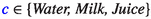• Objects with internal state: where and is the contained volume;

• Objects at graph-like locations: , where and are vertices of some graph;

• Stacks of objects: where is the count.

This allows us to easily add information to the resources. As compositions of processes use resources, requiring their equality wherever a connection is made, this information has an effect on what compositions are valid (see Sect. 4.4). For instance, with resource atoms located in a graph we can ensure that any movement of resources is done between adjacent locations.

Example

In the case of our running example, the vending machine, there are three kinds of objects we care about: cash, drinks and the machine itself. So, in that domain, these form our type of resource atoms with constructors , and .

To represent a single drink the constructor is sufficient and needs no parameter. But to represent some amount of cash we parameterise the constructor with a natural number—the amount of some currency is . Similarly for the vending machine itself, we parameterise the constructor with a natural number this time representing the amount the machine currently holds in credit.

Note that for simplicity we assume any amount of currency is one object rather than deal with denominations used in the real world. However, this model could be extended in a straightforward way to account for this detail.

The resource construction most relevant in this domain is parallel combination. For instance, if we have a vending machine with already in credit and want to buy a drink that costs , then we may start in the situation described by the following resource:

3.2 Parallel Resources as a Quotient

Resource terms give many ways of expressing the same resource. For instance, Fig. 3 shows syntax trees for five resource terms which express the same resource: the single atom A.

In our current formalisation we pay special attention to the variety of terms that can be produced by the parallel combination of resources. This is because parallel combinations arise frequently in our process combinations, and when they do it is often with more than two resources. As such, rendering the alternatives equal (see below) significantly simplifies building compositions at the price of a manageable increase to complexity of their mechanisation.

Other resource combinations can also produce a variety of terms, for example can be considered the same as . However, in our experiments, such equivalences lead to significant increase in mechanisation complexity with little gain in usability. For instance, in the given example, the resulting equivalence relation becomes more dependent on the contents of resource terms in addition to their structure. This in turn means we lose useful properties of resources, especially when it comes to systematically translating processes between domains.

For practical reasons, we consider the full integration of additional resource equalities into our framework as a future extension (see Sect. 9.1). However, although they are not resource term equivalences in the current formalisation, further resource transformations can be achieved through composition operators and resource actions (see Sects. 4.2 and 4.3) instead.

Fig. 3

Five parallel resource term trees expressing the same resource, the single atom A

In our formalisation of resources we collect all of the possible forms of a resource into one object. We first define an equivalence relation on terms and then form their quotient by that relation.

We inductively define the relation to relate terms that represent the same resource, as shown in Fig. 4. The first three introduction rules express the core of the equivalence, handling parallel combinations with no children, single child and nested parallel combinations respectively. Then the next seven introduction rules close the relation on the resource term structure, meaning the result will be a congruence. The final two rules make the relation on symmetric and transitive. The fact that it is reflexive, the last condition for it to be an equivalence, can be proven from this definition.

Fig. 4

Resource term equivalence

Now we can define resources as the quotient of their corresponding terms, treating each equivalence class as one object. This is easily done in Isabelle/HOL:

Because the relation is a congruence, meaning equivalent arguments to the same constructor yield equivalent results, it is also very simple to lift the constructors to the quotient. The lifting of definitions is automated by the Lifting package, introduced by Huffman and Kunčar [19]. Beyond the easier definition, this also automatically proves a number of useful facts relating it to the quotient and sets up code generation. For instance we lift the constructor as follows:

What is considerably more difficult is i) characterising the equivalence in a computable way and ii) recovering useful structure from resource terms for resources. The computable characterisation is particularly important, because without it we would not be able to generate code for anything involving resources. We discuss our solution to these two issues in the next two sections.

Before addressing those issues, we define an infix notation for parallel resources. This simplifies statements that involve few resources being in parallel. The resource product simply puts two resources in parallel:

Thanks to resources being a quotient this operation is associative and has as its left and right units. In other words, resources with this operation form a monoid.

Note that, once the quotient is made, it does not matter if we initially defined the parallel resource term combination as having arbitrary arity or as strictly binary. It only affects the phrasing of the equivalence rules, the normalisation procedure we use to decide that equivalence and the representation of resources in generated code. We choose to use lists because they more concisely reflect the monoidal nature of parallel resources and make for a simpler normalisation procedure.

3.3 Resource Term Normalisation by Rewriting

We give a computable characterisation of the resource term equivalence through a normalisation procedure based on the following rewrite rules:

(2)

(3)

(4)

(5)

The rules (2)–(4) are obtained directly from the introduction rules of the equivalence by picking a specific direction (see the first three rules in Fig. 4). The rule (5) is obtained from a theorem about the equivalence , allowing us to drop any resource within a one in a single step.

An alternative procedure, which normalises a term in a single pass, is described in Sect. 6.1. While that variant is more direct, and should thus be more efficient for computation, it is more difficult to use in proofs.

3.3.1 Normalised Terms

A resource term is normalised if:

• It is a leaf node (i.e. one of , or ), or

• It is a non-parallel internal node (i.e. one of , or ) and all of its children are normalised, or

• It is a parallel internal node (i.e. ) and all of the following hold:

  • All of its children are normalised, and

  • None of its children are empty or parallel resource terms (i.e. one of or ), and

  • It has at least two children.

We formalise this in Isabelle as the predicate through structural recursion on the type of resource terms:

3.3.2 Rewriting Relation

We define the rewriting relation, the congruence closure of the rules (2)–(5), as the inductive relation :

Note that this relation is reflexive rather than partial, so its normal forms are fixpoints rather than terminal elements. The rewriting step function (see Sect. 3.3.4) will have to be total, like all functions defined in Isabelle. By making the rewriting relation reflexive we can have the rewriting step function graph be a subset of this relations, which is useful for reusing proof.

As a form of verification, we show that a resource term satisfies the predicate if and only if it is a fixpoint of the relation . So these two definitions agree on what terms are normalised.

3.3.3 Rewriting Bound

The rewriting bound expresses the upper limit on how many rewriting steps may be applied to a particular resource term. For this bound we disregard many details of the resource term at hand in order to arrive at a simple definition, which means that even terms in normal form can have a positive rewriting bound—this is not the least upper bound. But there being a finite bound is sufficient to show that normalisation by this rewriting terminates.

We define the bound through structural recursion on the type of resource terms:

• If the term is a leaf (i.e. one of , or ), then its bound is 0.

• If the term is a non-parallel internal node (i.e. one of , or ), then its bound is the sum of bounds for its children.

• If the term is a parallel internal node (i.e. ), then its bound is the sum of bounds for its children plus its length (for possibly dealing with unwanted children) plus 1 (for possibly ending up with too few children).

The most crucial property we show is that for every term not in normal form this bound is positive. We also show that the rewriting relation does not increase this bound.

3.3.4 Rewriting Step

The rewriting relation given in Sect. 3.3.2 specifies all possible rewriting paths. When implemented, a specific algorithm must be chosen, which yields a rewriting function.

There are two choices when rewriting: the order in which we rewrite children of internal nodes, and the order in which we apply the rewriting rules. For an example of the latter: the term could be rewritten directly into by rule (3), or first into by rule (5) and only then into by rule (2).

Our rewriting algorithm is as follows:

• For the internal nodes and , always rewrite the first child until it reaches its normal form and only then start rewriting the second child if that one is not also already normalised.

• For the internal node we proceed in phases:

  • i. If any child is not normalised, then rewrite all the children (note that rewriting is the identity on already normalised terms); otherwise

  • ii. If there is some nested node in the children, then merge one up; otherwise

  • iii. If there is some node in the children, then remove one; otherwise

  • iv. If there are no children, then return the term ; otherwise

  • v. If there is exactly one child, then return that term; otherwise

  • vi. Do nothing and return the same resource.

We mechanise this algorithm in Isabelle/HOL via the function called , defined as follows:

We show that the graph of this function is a sub-relation of the rewriting relation. Thus normalised resource terms are exactly those for which this function acts as identity and the input resource term is always equivalent to the result.

Most crucial is that with this more specific formulation we can prove that, for any term not already normalised, this function strictly decreases its rewriting bound.

3.3.5 Normalisation

With this rewriting function the normalisation procedure is quite simple: keep applying as long as the resource term is not normalised. We mechanise this as the function and prove that it terminates by using the rewriting bound as a termination measure.

3.3.6 Characterising the Equivalence

In order to characterise the resource term equivalence we prove the following statement:

(6)

First, the $\Longleftarrow$ direction is simpler. We have already shown that every term is equivalent to the result of applying the rewriting step to it. Because the normalisation is repeated application of the step, by transitivity of the equivalence every term is equivalent to its normalisation. So two terms with equal normal forms can be shown equivalent using transitivity and symmetry of the resource term equivalence.

Second, the $\Longrightarrow$ direction is more complex. It relies on showing that equivalent resources are joinable by the rewriting function, meaning there is a sequence of rewrite steps from each term to some common (possibly intermediate) form. We formalise this statement by casting the rewriting step in the language of the Abstract Rewriting [41] theory already mechanised for the IsaFoR/CeTA project [42] and available in the Archive of Formal Proofs.² We prove it by induction on the resource term equivalence, where for each of its introduction rules we prove that such joining rewrite paths exist.

Now, we already know that every term is equivalent to its normal form. So, by transitivity and symmetry, normal forms of equivalent terms are themselves equivalent. Then, by the joinability rule we just showed, we have that these normal forms are joinable. But, because they are normalised terms, we know that each only rewrites to itself. Therefore the form that joins them can only be those normalised terms, and so they must be equal.

As a result we get a computable characterisation of the resource term equivalence . We add equation (6) to the code generator, meaning that Isabelle/HOL is no longer blocked from generating code for anything involving resources. This characterisation is also important to how we translate resources into linear logic in Sect. 5.2.

3.3.7 Representative Term

Now that the resource term normalisation is verified, we can use it to define a representative term for every resource. While every resource is an equivalence class of terms, there is exactly one normalised term among them. We denote the representative of as . Having such a representative is useful, for instance, for visualising the resource.

The representative can be constructed by applying the rewriting normalisation procedure to any term in the class. As with the resource constructors (see Sect. 3.2), this definition is facilitated by the Lifting package [19].

Thus, we define to be the normalisation procedure but with resources as its domain. This requires that normalised terms be equivalent, which they are.

We can check this by proving the following, where is the equivalence class representing and chooses an arbitrary that satisfies :

3.4 Resource Type is a Bounded Natural Functor

When modelling processes in a certain context, the resources are built from available resource atoms. It is then useful to have a method for systematically changing the content of a resource (the resource atoms it contains) without changing its shape, translating the resource from one context to another. In general, such a method is called a mapper [13].

Suppose, for instance, that we were using a specific currency in our vending machine example, say British pounds. Then we may want to map a process from that domain to one using US dollars instead. We would do that by taking every resource in the process and systematically applying the currency conversion to all atoms the resource contains. The mapper generalises this operation for any function on resource atoms. For another example, we use the process mapper (and by extension the resource mapper) in Sect. 7.5 when combining two domains into one.

For resource terms, Isabelle/HOL automatically defines the mapper and proves its properties (e.g. that it respects the identity function and commutes with function composition). This is because every inductive datatype in Isabelle/HOL is a bounded natural functor (BNF), a structure for compositional construction of datatypes in HOL presented by Traytel et al. [43] and integrated in Isabelle/HOL by Blanchette et al. [6]. It therefore remains for us to lift this term-level mapper to the quotient and transfer its properties.

Fortunately, lifting the BNF structure from a concrete type to a quotient has been automated by Fürer et al. [13] who reduce this task to two proof obligations concerning the equivalence relation being used and parts of the BNF structure of the concrete type. Once these obligations are proven, the constants required for the BNF structure of the quotient and their properties are automatically derived.

The first obligation concerns the relator, an extension of the mapper to relations on the content instead of functions. It ensures that the generated relator will commute with relation composition. While its proof would usually be quite difficult, Fürer et al. describe how this condition can be proven using a confluent rewriting relation whose equivalence closure contains the equivalence relation we used to define the quotient type. In our case, the resource term normalisation procedure described in Sect. 3.3 gives us exactly such a relation.

The second obligation concerns the setter, which gathers the content into a set while discarding the shape. It ensures that the generated setter will be a natural transformation, that is applying the setter after mapping a function is the same as using the setter first and then applying that function to every element of its result. In our case this condition can be proven using structural induction on resource terms and Isabelle’s automated methods.

As a result we get the BNF constants (mapper, relator and setter) and properties, all already integrated with the automated tools within Isabelle.

4 Process Compositions

With resources formalised we now move to compositions of processes over them. Process compositions are about describing individual actions in terms of what resources they consume and produce, and how those can be put together to form larger processes.

Since resources may be physical objects we must be careful to handle them correctly, so that none are used twice or discarded without justification. We call this linearity. In Sect. 5, we describe how we formally verify that these compositions obey the rules of linear logic and so handle resources correctly.

We mechanise process compositions as the datatype , with type variables for resource atoms, for labels and for other metadata:

This datatype captures a complex process as a tree of composition actions applied to simple processes. In the rest of this section we describe the nodes of the process composition trees in more detail, including their input and output resources (also shown in Fig. 5), and discuss the correctness conditions on compositions.

Note that in text we use the notation to say that process has input resource and output resource . Recall also that in Sect. 3.2 we defined as infix syntax for . So, we have for instance: (see Sect. 4.3).

Fig. 5

Process composition tree input and output

4.1 Primitive Actions

We start with primitive actions which depend on the domain we are modelling: they represent things we can do in the domain. For instance, if the domain has a notion of resources with locations, then there will be some kind of movement action which may move an object freely between locations or be constrained to edges of some graph. We treat these as assumptions of the model.

In Isabelle/HOL, we represent a primitive action by , where and are its input and output resources respectively, is its label and is any other associated metadata.

The label serves to distinguish actions that may have equal inputs and outputs but different meaning, such as two modes of moving an object between locations with different costs and speeds (e.g. walking vs. running). The term “label” is used because it is often set to a printable type, such as a string, which we then use as a label in visualisations (particulars of process visualisation are not discussed in the present paper). The metadata can carry any further information we may wish to associate with the primitive actions, such as cost of execution or parameters for implementation (see for instance its use in Sects. 7.3 and 7.5).

Both the label and metadata are taken from arbitrary types (the unconstrained type variables and of ) so they can carry any kind of complex information.

Recall that these primitive actions correspond to the assumptions about the domain on which the composition relies. We make it convenient to collect the assumptions by defining the function with the following signature:

It gathers the parameters of every node, returns the empty list for every other leaf of the composition and gathers children’s results for every internal node using list append.

Example

In our running example, the vending machine, we have three primitive actions: paying into the machine, getting a drink and getting change. We use string literals as labels and assign no metadata to these actions (by using the constant of type ).

Paying money into a vending machine requires the machine, which can hold an amount of existing credit, and the cash being paid in. It produces a machine with the combined amount in credit. We define the action as a function of the two variables:

Returning funds from a vending machine only requires a machine and it produces a machine with zero credit left and the relevant amount of cash dispensed:

Getting a drink requires a machine with credit of at least the price of the drink and produces a machine with decreased credit and the drink. We define this action as a partial function of the price and credit:

Note that we separate the actions of getting a drink and returning change, while often vending machines return change automatically along with the purchase. Our formulation separates these two concerns, which allows returning change and cancelling to both be handled by the action.

4.2 Composition Operators

Next we have four ways of creating processes from one or two simpler ones, allowing us to inductively describe how to orchestrate the primitive actions:

• Sequential composition—

  First execute and then use its outputs to execute .

• Parallel composition—

  Execute and concurrently, but combine their inputs into one parallel resource and the same for their outputs.

• Optional composition—

  Take as input the non-deterministic combination of inputs of and , executing exactly one of them based on the branch of the input that is supplied at runtime. This serves as the only way to eliminate the non-determinism, so it requires that and have the same output resource.

• Representation—

  Introduce the executable resource representing , which could be a composition in its own right. This requires no input, analogously to a constant being viewed as a nullary function. Note that the output could have been defined as not copyable, but based on experience with modelling processes we decided to make the output explicitly copyable. This means we do not have to know ahead of time how many times we intend to use the representation.

The simplicity of these composition operations may seem restrictive. For instance, what if we wish to use only part of the output of as input to , essentially using to further process some objects produced by while keeping others untouched? In such a case our composition operations require us to state this explicitly so there is no ambiguity: do and then do concurrently with “doing nothing” for an appropriate subset of ’s outputs. This way process compositions (motivated by linearity) approach the frame problem [25]: the lack of change must be stated, but it is easy to do so automatically. The ways in which we express such lack of change are discussed in the next section.

Example

Perhaps the simplest process composition in our running example is paying money into a vending machine and then getting a drink. For example we can pay 10 into an empty machine and then get a drink costing 5 from the machine which then has 5 left as credit:

4.3 Resource Actions

Expressing concepts such as “doing nothing” is where resource actions come in. These are similar to primitive actions but, instead of expressing an assumption about some particular domain, they express things we can always do with resources.

As an inspiration for this range of actions we use theorems of linear logic: if an action can be argued in linear logic without making any assumption about the domain, then we can consider it as always doable with resources. Note that to argue for some of these actions one needs more than one inference rule, such as with OptDistrIn and OptDistrOut. We aim for convenience of expressing process compositions more than for atomicity with respect to the logic.

The resource actions are as follows:

• 

  Take any resource and produce it unchanged. For instance, to keep a resource aside while doing something with other resources.

• 

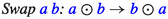
  Swap the order of any two parallel resources. This allows us to compose processes when their interface has the same resources but in different order, while retaining information about how they were reordered.

• and

  Take one resource to its non-deterministic combination with another. For instance, if a process has input and we can deterministically obtain from another process , then is the bridge that connects from to . Furthermore, injections in combination with Opt can also be used to optionally compose³ any two processes and to one of the form .

• 

  Distribute a parallel resource into both branches of a non-deterministic one. This is useful when is deterministically available but needed to resolve the branches of . For instance, if always available tools are needed to repair a machine that may break during its use.

• 

  Distribute a parallel resource out of both branches of a non-deterministic one. This is useful when processing some non-deterministic resource produces a partially deterministic result. For instance, if using a machine may result in a successful or failed product but always also outputs the machine itself. (Note that this action could be defined as a composition of others⁴, but we keep it as a primitive for convenience and symmetry.)

• 

  Discard the copyable marker from a resource to use it in a process that does not assume its copyability. This is particularly useful to evaluate a copy of the executable resource produced by representing a composition.

• 

  Duplicate a copyable resource into two copies. For instance, to use a single password input for multiple actions requiring it.

• 

  Discard a copyable resource, producing nothing. For instance, when an action produces a digital alert to which we do not wish to react.

• 

  Take any resource and an executable resource with matching input, evaluate the process represented by the latter and produce its output. If we use a process to prepare an resource, then this allows us to execute it.

• 

  Forget all information about some resource, producing . For instance: if we have a drawer with socks of two colours, then we can specify the output of a process that finds two matching socks more concisely as: (for more on this sock example see Dixon et al. [12]). Note that what is forgotten are details about the resource and not its presence, only copyable resources can be erased.

Because these actions are defined regardless of the resource atoms we choose to use, and because those atoms can be of any type, none of the resource actions could possibly interact with the internal state of atoms. They do not change the objects themselves, only how they are arranged. We refer the reader once more to Fig. 5 for the formal definitions of inputs and outputs of all the resource actions.

Example

With resource actions we can follow paying money in and getting a drink with a refund of the remaining credit as change. We do this by following the previous composition with refunding in parallel with identity on the drink, defined formally as follows and visualised in Fig. 6:

Fig. 6

Process diagram of paying into a vending machine, getting a drink and the remaining change

4.4 Valid Compositions

While building compositions of processes, we wish to ensure that we are doing so sensibly, in particular that we are manipulating resources correctly. We call such process compositions valid.

One approach would be to perform each step as a deduction in linear logic. However, this would limit the concepts we can express in compositions and their validity to only what we can express within linear logic.

Instead, we set up rules purely in the language of resources about what compositions “make sense”. We then prove (Sect. 5.6) that the mechanical translation of any composition into a linear logic deduction will be well-formed if the composition satisfies these rules. This approach yields conditions simpler than the full rules of linear logic. The decoupling allows us to potentially extend validity with conditions beyond what linear logic can express, allowing our framework to extend beyond linearity.

There are only two non-trivial rules:

• In sequential composition , the output of the first process must be the input of the second process .

• And in optional composition the outputs of both processes must be equal, so that no matter the branch actually taken we know what the output will be.

We call a process composition valid when it satisfies these rules everywhere within it, and we define this predicate in Isabelle/HOL as shown in Fig. 7.

Fig. 7

Process composition validity

As an example consider processes , with output , and , with input , and . The sequential composition of then is not valid, because the output of is not the input of . However, by composing in parallel with identity processes on and we can “fill out” its output to make the sequential composition valid. This situation is visualised in Fig. 8.

Fig. 8

Example of how sequential composition can fail to be valid, visualised through process diagrams

Validity ensures that resources are only changed as explicitly stated by actions. Furthermore, composition operations and resource actions at most manipulate the structure of resource combinations and not their contents, to which they do not have access. The only way to change information in resource atoms is via primitive actions, which are all assumptions about the domain. As a result, the information within resource atoms can interact with this notion of composition validity in interesting ways.

Example

On top of the basic connections making sense, validity in our running example ensures that the amount of cash and the amount paid into a machine do not change between actions. By inspecting the primitive actions we use, we can also see that money either moves between the machine and cash, through paying in and refunding, or it is turned into drinks.

Another implication of validity in this domain is that every instance of getting a drink is possible. This is because the action definition is partial, only giving a process for machines that have enough paid in. Thus if we can prove a composition is valid, then every instance of getting a drink within it must have been defined and must have had a machine with enough paid in supplied to it. This rests on the fact that it is impossible to prove that the value is a valid composition.

5 Translating into Linear Logic

In this section we describe our argument for the linearity of resources in process compositions, connecting the compositions to deductions in ILL (see Sect. 2.1).

The argument is, in short, that every composition corresponds to a deduction in ILL with the following properties:

Well-formedness:

For every valid composition the corresponding deduction is well-formed: it follows the rules of ILL.

Input-Output Correspondence:

The conclusion of the deduction is a sequent $I \vdash O$ where I and O are propositions corresponding to the composition’s input and output respectively.

Primitive Correspondence:

Primitive actions of the composition correspond exactly to the premises of the corresponding deduction.

Structural Correspondence:

The structure of the composition matches that of the corresponding deduction.

To express the above, we must embed ILL in Isabelle/HOL. We first mechanise a shallow embedding, allowing us to formally talk about what sequents are valid in the logic. But this is not enough to demonstrate the above properties, so we also mechanise a deep embedding which allows us to formally talk about the deductions themselves and their structure. We prove that the deep embedding is sound and complete with respect to the shallow embedding. We refer the reader to the work of Dawson and Goré [11], for instance, for a further discussion of shallow and deep embeddings in Isabelle/HOL.

When connecting resources to ILL propositions we encounter a difficulty in the many concrete terms that may represent one resource. To resolve this we use the normal form and mirror the rewriting normalisation procedure (see Sect. 3.3) with ILL deductions to show that any equivalent resource terms correspond to logically equivalent propositions.

Note that the connection is from process compositions to linear logic deductions, but not necessarily the other way. There exist well-formed ILL deductions which do not reflect any of our process compositions, for instance because we do not make any connection to the ILL operator. Similarly, the resources and process compositions may be extended to carry information that cannot be expressed in ILL.

5.1 Shallow Embedding of ILL

A shallow embedding of ILL is simpler to define than the deep one and it allows us to reuse much of the automation available in Isabelle. However, it is limited to formalising what sequents are valid within the logic rather than directly talking about the structure of its deductions.

There is already a shallow embedding of ILL by Kalvala and de Paiva [21] distributed with Isabelle, but this is part of the Isabelle/Sequents system and is not compatible with our HOL development. Nevertheless, their approach provides inspiration for some aspects of our mechanisation.

First we mechanise the propositions of ILL as the datatype , mirroring the specification (1), given in Sect. 2.1, along with relevant notation. The type variable represents the type from which we draw the propositional atoms.

Then we represent the valid sequents of ILL as an inductive relation between a list of propositions (antecedents) and a single proposition (consequent). We denote it infix by and the full definition is shown in Fig. 9.

Fig. 9

Shallow embedding of valid ILL sequents

Every rule in this definition represents one of the inference rules of ILL shown in Fig. 2. However, we adjust their precise statement following the work of Kalvala and de Paiva [21] to remove implicit assumptions which make them less useful for pattern matching. For instance we adjust the $\otimes _L$ rule by adding $\Delta$ so that we no longer assume that A and B are the last antecedents:

Note that, compared to our statement in Sect. 2.1, ILL is often stated with multisets for antecedents instead of lists as in our formalisation. In such contexts the order of antecedents does not matter and the structural inference rule Exchange is made implicit.

With our shallow embedding of ILL (using explicit Exchange, see in Fig. 9) we can prove that this move is admissible in the logic. We do so by proving that any two sequents whose antecedents form equal multisets are equally valid, stated more generally in Isabelle as follows:

This fact relies on the theories of multisets and of combinatorics already formalised in Isabelle/HOL. We first note that any two lists forming the same multiset are related by a permutation, which is a sequence of element transpositions. By induction on this sequence of transpositions we show that we can derive each sequent from the other.

5.2 Resources as Linear Propositions

Before relating process compositions to ILL deductions we first need to relate the resources within the former to ILL propositions. Then we can translate the input and output of processes into ILL.

Because resources are defined as a quotient, we first define the translation for resource terms:

Note how all but the case map a resource term constructor directly to a constructor of ILL propositions. The case instead uses the helper function to combine the list of translations of the children using the binary operator of ILL. This function is defined as follows:

Then we extend this to resources by translating the normal form representative term obtained via (see Sect. 3.3):

The crucial property of this translation is that for equivalent resource terms the translation of one can be derived from the translation of the other within ILL. So the logic agrees with the relation we defined. In our shallow embedding this is stated as follows:

with the reverse derivation following by symmetry of resource term equivalence.

In the translation of process compositions to deductions we may construct translations of non-normal terms, so this property is vital to the resulting deductions being well-formed. Consider a situation that may arise from parallel composition of a process with two inputs, say and , with a process with one input, say :

• The combined input is which translates to .

• But the first input is , which translates to , and the second input is , which translates to .

• The product of those translations is which is not the same proposition.

We prove the property by induction on the resource term equivalence relation. In each case we use Isabelle’s automated methods to find the deduction pattern needed to transform one translation into the other. These methods make use of facts about ILL as well as facts about the proposition compacting operation, such as the following:

5.3 Shallow Embedding is Not Enough

With the shallow embedding of ILL we can start formalising our argument for linearity of process compositions. In this section we describe how this embedding allows us to demonstrate the Well-formedness and Input-Output Correspondence properties and how it is insufficient for the Primitive Correspondence and Structural Correspondence properties. This insufficiency motivates our use of a deep embedding in the following sections.

For every process composition , we have the following ILL sequent formed from translating its input and output (call it the input-output sequent):

We can show that, for every valid process composition, its input-output sequent is valid in ILL given the validity of input-output sequents of primitive actions occurring in the composition (call this the shallow linearity theorem):

We prove this statement by structural induction on the process. In each case we make use of Isabelle’s automated methods to find an ILL sequent derivation from the translation of the input to the translation of the output.

The Well-formedness property is demonstrated by the proof being checked by Isabelle, while Input-Output Correspondence is demonstrated by the conclusion being the input-output sequent of the composition.

Primitive Correspondence is not sufficiently demonstrated by this theorem. Its assumption only says that input-output sequents of the primitive actions are sufficient for the proof. This does not necessarily mean that they are necessary nor that they are used as many times as the primitive actions occur in the composition. Thus we cannot conclude that the primitive actions correspond exactly to the premises of this deduction.

Structural Correspondence is also not demonstrated by the theorem. The structure of its proof does not necessarily follow the structure of the composition. We know that there exists some proof of the input-output sequent, but that proof may not have any further relation to the composition itself and so this is not a satisfying argument for its linearity.

Consider for example process compositions whose input is equal to their output. We can prove the input-output sequent for any such composition to be valid in ILL directly by the Identity inference rule:

In this way, the sequential composition of primitive actions and then can have its input-output sequent shown to be valid in ILL without using any premise at all.

Moreover, consider the sequential composition of identities on resources , then on and then again on (where and are distinct). Its input-output sequent can again be shown to be valid in ILL, despite this composition being invalid because it creates and discards the resource .

In the following sections we develop a deep embedding of ILL deductions which allows us to demonstrate the Primitive Correspondence and Structural Correspondence properties. With the deep embedding we can say that ILL accepts not just the input and output of a process composition but every step within it.

5.4 Deep Embedding of ILL

A deep embedding of ILL deductions produces “objects” we can directly construct. While this gives up much of the automation that Isabelle would offer during proof, it allows us to build deductions whose structure matches the process composition.

For this, we mechanise the deductions as the datatype . Elements of this datatype are trees whose nodes exactly mirror the introduction rules of the sequent relation (see Fig. 9), with an additional node for explicitly representing premises (the meta-level assumption of a particular deduction). This additional node lets us express contingent deductions.

The type of deductions is parameterised by two type variables: and . The type represents the type from which we draw the propositional variables, just as it does in the type of propositions. The type represents the type of labels we attach to the premise nodes. We use these labels to distinguish premises that may assume the same sequent but have different intended meaning.

In total this datatype has 22 constructors, each with up to eight parameters. The deduction tree’s semantics are defined via two functions: expresses the deduction’s conclusion sequent while the predicate checks whether the deduction is well-formed. Full definitions are shown in Appendix A, but as an example we consider the Cut rule which is stated in the shallow embedding as follows:

Its deep embedding, the term , represents the deduction tree shown in Fig. 10. Note that and correspond to deep embeddings of the two assumptions in the shallow rule: and respectively.

Fig. 10

Deduction tree represented by the term

The semantic functions take the following values for this rule:⁵

Additionally, a function called recursively gathers the list of all the premise leaves in a deduction. Continuing the above example, the premises of a cut node are those of its two child deductions:

We verify this deep embedding by proving it is sound and complete with respect to the shallow one. Soundness requires that the conclusions of well-formed deductions are valid sequents given the validity of the premises, stated in Isabelle as:

Completeness requires that for every valid sequent there exist a well-formed deduction with it as conclusion and with no premises:

Because the deduction tree nodes mirror the sequent relation introduction rules, we can prove these statements rather simply by induction either on the deduction structure or on the sequent relation. Note that for completeness we require the deduction to have no premises because otherwise it would be trivial: we could just assume the sequent.

5.5 Deeply Embedded Equivalence of Resource Translations

In Sect. 5.2 we proved that translations of equivalent resource terms can be derived from one another:

We use this fact to fill gaps between linear logic translations of different but equivalent resource terms, which will be vital when we construct deductions from process compositions in the next section. To make use of this fact in the deep embedding, we first need to describe how a witness deduction is constructed for every case. This mirrors the earlier problem of deciding the resource term equivalence, so our solution is similar to the normalisation procedure described in Sect. 3.3.

We build a deduction from one resource term to its normal form and another deduction into the other term from its normal form (note the opposite direction). These two deductions can then be connected because the two terms have equal normal forms. Thus the core of our solution are two functions which construct, for any term , the deductions with the respective conclusions:

In the definitions of these functions we again mirror the normalisation procedure. However, instead of a rewriting step that transforms the resource term, we build a deduction (in the desired direction) proving the transformation is allowed in ILL. These are then chained with the Cut rule until the resource term is normalised.

We prove that these functions in all cases produce well-formed deductions with the above conclusions. Furthermore, we prove that they have no premises and are thus theorems of ILL.

We name the two functions and : ILL deductions that connect a resource term from or to its normal form. They are used in the next section when constructing deductions from process compositions to fill gaps between linear logic translations of different but equivalent resource terms.

5.6 Process Compositions as Linear Deductions

With the deep embedding of ILL deductions we can prove the shallow linearity theorem from Sect. 5.3, which states that the input-output sequents of process compositions are valid in ILL. But now, we can do so in a way that satisfies the Primitive Correspondence and Structural Correspondence properties which we identified in Sect. 5, namely that: premises of the deduction correspond exactly to the primitive actions of the composition and the deduction matches the process composition in structure.

We do this by recursively constructing an ILL deduction for every process composition, mechanised as the following function

By associating every constructor of process compositions with a pattern of ILL inferences, this function ensures that the resulting deduction reflects every step of the composition.

We then prove that the resulting deductions demonstrate the Well-formedness, Input-Output Correspondence and properties. That is, we show that for any valid process composition the deduction is well-formed:

and the conclusion is always the input-output sequent:

and that the premises correspond to the primitive actions that occur in the composition (including in number and order):

By the soundness of the deep embedding (see Sect. 5.4) each thus constructed deduction is then a proof for an instance of the shallow linearity theorem from Sect. 5.3 but with added guarantees about the proof’s structure.

We next outline precisely how constructs the deductions. In some cases the translation is direct, for instance and are translated into premises and identity rules respectively:

In other cases the deduction being constructed may be more complex, especially where different forms of one resource are involved. For instance with parallel composition we need to:

• 1. Separate the proposition translation of a parallel resource into translations of the two inputs,

• 2. Use the children’s deductions to connect translations of their inputs with translations of their outputs.

• 3. Merge the translations of the two outputs back into one proposition for the combined resource.

In Isabelle/HOL we define this case as shown in Fig. 11a and visualised as a proof tree in Fig. 11b. The Isabelle/HOL definition uses helper functions for a frequent instantiation of the Cut rule and to juxtapose two deductions using the $\otimes _R$ and $\otimes _L$ rules, and the connections between a resource term and its normal form.

Fig. 11

Witness of linearity for parallel composition

Thus we have fully mechanised our goal with this translation. We show that all valid process compositions are linear on the grounds that they obey rules of linear logic by mechanically producing the specific ILL deduction witnessing this fact. Further, because the way we construct this deduction involves no proof search, we can have Isabelle/HOL generate executable code for it and construct the witness even outside of the proof assistant.

6 Generation of Verified Code

Not all uses of our framework can be fully formalised in a proof assistant. This is particularly true where side-effects are concerned, such as drawing a diagram for a process composition into a file.⁶ For such uses we integrate with other programming languages by having Isabelle/HOL generate formally verified code for our definitions. Its code generator [15] can export code in SML [28], OCaml [23], Haskell [36] and Scala [30]. We currently use the Haskell generation.

Isabelle can set up the code generation automatically for the vast majority of our definitions. However, our resource term equivalence relation is defined inductively (see Sect. 3.2) and must therefore be given an alternative characterisation.

In Sect. 3.3 we introduce a procedure for resource term normalisation based on rewriting, which we show satisfies the inductive specification. This gives a computable characterisation to the resource term equivalence, but may be inefficient.

In this section we will start by describing an alternative procedure for resource term normalisation; one optimised for faster computation at the cost of its usability in proofs. We prove the two normalisation variants equivalent, so we can pick which definition to use based on which best suits the situation.

Then we describe how we actually generate Haskell code from our mechanisation. While our discussion here focuses on resource term normalisation, the same approach generates executable code for the whole of our formalisation. We use the generated code, for instance, to produce the mechanical instructions for implementing process compositions in Sect. 7.7.

6.1 Direct Resource Term Normalisation

The resource term normalisation procedure in Sect. 3.3 gives a computable characterisation of the resource term equivalence in a format suitable for inductive proofs. This is important to our mechanisation of resources and for their translation into ILL (see Sect. 5.5).

But there is a more direct way the normalisation can be done, one that produces more efficient code. This direct procedure normalises a resource term in a single pass from the bottom up with the aid of three functions.

The first two functions are related: they take a list of resources, intended to be the children of a node, and simplify that list by removing any terms it contains and merging up any nested terms it contains. We define them as follows:

The third function takes a list of terms and merges them in a way equivalent to what the constructor would do. However, it simplifies the result when the input list is empty or has only one element. We define it as follows:

The combination of these three functions comes in when simplifying regions of parallel resource combinations. Once we have normalised all the children of a node, we run them through the first two functions to simplify this node. Then we put them together with the third function, which takes care of cases that can be simplified even further.

The definitions of these three functions are rendered quite simple by intending them for a list of terms that are already normalised. This gives us strong assumptions about the elements, such as the fact that no terms in the list will contain further terms. The full direct normalisation procedure is then as follows:

Just as with the rewriting variant (see Sect. 3.3) we prove that this procedure produces normal forms and that for normalised resources it acts as identity. Most crucially, we prove that this procedure also characterises the resource term equivalence:

We can also verify, more precisely, that the two normalisation procedures give equal normal forms. With this fact we can instruct Isabelle to automatically replace references to in generated code with references to .

6.2 Haskell Code Setup

We now briefly outline how Haskell code is exported from our theory. This is split into an Isabelle theory that defines what to export and a Haskell Stack⁷ project with a package to contain the generated code.

First part is an Isabelle theory file where we define what constants should be exported and how. We export the main constants for every part of our framework including, among others, operations on resources and process compositions as well as their translations into ILL. Note that Isabelle automatically includes any constants that these definitions use.

Into this theory file we also import the theory distributed as part of Isabelle/HOL. This sets up natural numbers and integers to take advantage of the native Haskell type Integer instead of their fully formal definition, thus simplifying the generated code.

Here we also instruct Isabelle to replace all references to the rewriting variant of resource term normalisation (see Sect. 3.3) with the direct variant (see Sect. 6.1). This relies on us having proven these two variants to be equal.

Second part is the package that will contain the generated code and make it available as a library, which is part of a larger Haskell Stack project. This package keeps the formally verified code separate from code that uses it, clearly outlining what is reliable, but makes it easy to build on top of it. With it we can implement applications of our framework that may not be tractable to formalise in a proof assistant, such as visualisation. In Sect. 7.7 we discuss another such application: generating instructions for implementing a process composition in a particular domain.

When building the Isabelle theories we have it export the generated Haskell code into the source directory of this package. This is simple to achieve with a handful of parameters to the Isabelle build system and the whole process can be automated with a shell script.

7 Case Study: Formalising Balanced Manufacturing

We now demonstrate how we can use our framework to formalise solid manufacturing in the logistics simulation game Factorio.⁸ Its notion of manufacturing fits well with our notion of processes with inputs and outputs, and its simulation engine offers a way to implement a process and validate its properties in an idealised situation.

This game has previously been used to simulate logistics and process performance. Reid et al. [39] use it to formulate the logistic transport belt problem, which concerns the optimal placement of logistic elements to transport items between locations in the presence of obstacles. Boardman and Krejci [7] use Factorio as a simulation and visualisation aid in lessons about production and inventory control.

We start our discussion with the motivation for the formalisation choices for this domain. Then we discuss our formalisation of item flows and their logistics actions. We then extend this domain with machine blocks, allowing us to express manufacturing. With all of these defined we can start forming process compositions, exemplified with a specific manufacturing process. Then we discuss a Haskell program, based on code generated from these definitions, that constructs instructions for implementing these compositions in the game. Our model of this domain relies primarily on parallel combinations of resources, so we conclude with a short discussion of domains where the other resource combinations would be useful.

7.1 Problem Setup

We represent manufacturing in Factorio as process compositions, taking a steady state perspective. This means representing the average performance over an infinite period of observation. For instance, if a machine takes five minutes to finish an operation and produces 600 units, then we would treat it as having an output rate of 2 units per second. This is natural in Factorio: we build factories that continually transform inputs into outputs without player intervention. The same steady state perspective is also taken by various user-developed assistants, such as Helmod⁹ and Factory Planner.¹⁰

We want the validity of a composition to ensure that the process is perfectly balanced. This means that all connected input and output rates match throughout the process. As such, one kind of object is so-called “item flows” which represent the arrival of some amount of certain item type per second.

Beyond the rate of production and consumption, we also want the compositions to contain information about the required logistics connections, i.e. how items move between locations. Thus we include location as part of item flows to represent where the items are arriving. Note that representing locations by precise coordinates would make our models overspecified, so we instead use abstract named locations. The precise layout of machines and routing of logistics is left to the agent (human or AI) implementing the process.

Finally, the compositions should also account for the machines taken up by the manufacturing. Because in this domain we often use large numbers of machines, we use “machine blocks” to represent groups of machines performing the same recipe in parallel from common input flows into common output flows. These machine blocks integrate with logistics through these input and output flow locations.

We first define a domain with just item flows as resource atoms (see Sect. 7.2) and primitive actions that represent logistics: splitting, merging and moving the flows (see Sect. 7.3). Then we extend this domain with machine blocks as further resource atoms (see Sect. 7.4), which allows us to represent manufacturing with a primitive action in the combined domain (see Sect. 7.5).

As an application of the process models, we define how a sequence of specific instructions for their implementation in the game can be generated for every valid composition (see Sect. 7.7). By mechanically following these instructions a player can implement the process. If the machine and logistics layout problems are solved, then an automated agent could also be made to mechanically follow these instructions.

This last part builds a text output (see Listing 1 in Sect. 7.7) based on the given composition, so there is little we could gain by formalising it in Isabelle/HOL. We instead implement it in Haskell on top of the formally verified code generated from the formalisation of this domain.

7.2 Item Flows

We start our formalisation of this domain by defining located flows of items. Location names are string literals:

We only need locations to be uniquely identified. We choose to use string literals, rather than numeric identifiers, because they are more convenient when for example printed as part of the instructions. The same reasoning applies when using string literals for action, item and machine labels in the rest of this section.

Item types are defined simply by their label, for instance an iron plate:

and item flows are then built from the item type, flow rate and location:

Note that the flow rate is a rational number ( in Isabelle/HOL). Rational numbers are sufficient to express rates and, compared to for instance the reals, their formalisation has a simple translation into executable code in the form of fractions.

Because we will often be expressing item flows as individual resources, we define more convenient Isabelle notation for them:

stands for:

7.3 Logistics Actions

We have five primitive actions representing logistics, each associated with the following information:

• Merging and splitting flows: shared item type and location, and the two rates of flow;

• Creating and discarding an empty flow: item type and location;

• Moving a flow: item type, rate of flow, origin and destination.

Before defining the actions themselves we specify the metadata they will carry. In general, we use this data to support applications that inspect or consume compositions. In this case, the application is the construction of a sequence of instructions for implementing the process. Thus our metadata carries the information the user needs to implement each action.

We formalise the metadata for actions on item flows in Isabelle/HOL as the inductive datatype :

With metadata set up we can define the actual primitive actions, using item flows as resource atoms, string literals as action labels and the above as metadata.

We define the splitting, merging and moving of item flows as follows:

where, for instance, a action takes two flows of the same item at the same location but with different rates and , and produces one with item and location unchanged but with summed rate. The split action does the opposite and the action changes only the location. See Fig. 12 for example diagrams of these actions.

Fig. 12

Process diagrams for example instances of , and actions

We also assume that we can create and discard zero-rate flows for any item, defining the unit and counit actions:

7.4 Machine Blocks

Before we can consider manufacturing actions we need to formalise machines and machine blocks, so that we can add them to the resource atoms.

Machines are defined by their name, processing speed, and idle and running energy demand:

such as the electric furnace that processes items at double of base speed, consumes $6\ kW$ of power while idle and an additional $180\ kW$ while running:

Note that the machine processing speed is again a rational number to allow for machines taking more than base time (i.e. speed less than one). The two energy demands, one when the machine is idle and one when it is running, are both natural numbers representing watts.

Machine blocks are built from the machine, count, and input and output location:

As with item flows, we define more convenient Isabelle notation for machine blocks as individual resources:

stands for:

7.5 Manufacturing Action

The basis of manufacturing in our formalisation is the action of performing some recipe, using a block of machines to convert one set of item flows into another.

Recipes are defined by two lists of item–count pairs (one for the inputs and one for the outputs), the time and machine required and a name:

such as crafting one iron gear from two iron plates:

Performing a recipe with some number of machines in parallel requires flows of its inputs at one location and produces flows of its outputs at another location. We define a function to help us construct these flows:

which takes the recipe’s time requirement , machine block location , number of parallel machines running the recipe, their processing speed , the item and its count , and constructs the corresponding item flow. The last two arguments being taken as a pair is important to make this function suitable for mapping over the item–count lists with which recipes are defined.

The final piece of preparation is the metadata, which in this case collects the recipe, number of parallel instances, input location and output location:

To express manufacturing actions, we move into a domain that combines both item flows and machine blocks. This means that our processes now use as resource atoms the sum of those two types: . Similarly, as metadata they use the sum of item flow and manufacturing metadata: . The two constructors of Isabelle’s sum type, which inject a value from either summand into the sum type, are and .

The manufacturing primitive action can then be defined as follows:

where the input resource is a parallel combination of item flows—one for each input item of the recipe—along with a suitable block of machines. The output resource is a parallel combination of only the item flows for the recipe’s outputs. The function merely projects the second argument from the constructor, its processing speed.

Figure 13 shows an example diagram of the action. It takes as input three item flows of the recipe ingredients (iron gears, iron plates, steel plates) arriving at the location named “Source” and the two assembling machines used to perform the recipe. Those machines take inputs from “Source” and deposit their products at another location named “Destination”. See Fig. 14 for further instances of this action.

Fig. 13

Process diagram for crafting cargo wagons on two machines in parallel

The machine block is consumed by this action to represent occupying those machines with continuous production. This prevents us from using the same group of machines for two tasks at the same time. The block’s locations are set to match those where the input and output flows are generated, and its size is set to match the multiplier used to compute the flow rates.

With all the primitive actions set up we can proceed with constructing compositions. In the following two sections we describe one such composition and describe how instructions are mechanically generated from such compositions.

From this point on we work in the combined domain, so we redefine our custom notation to use the appropriate injections. The item flow notation and the machine block notation now apply and respectively before constructing the resource atom.

Note that all processes from the item flow domain can be easily translated into the combined domain. We just apply the left injection constructor to all resource atoms and metadata through the process map: . This map is defined automatically by Isabelle thanks to the BNF structure of resources (see Sect. 3.4).

7.6 Example Composition: Four Iron Gears

As an example composition we consider the process of turning iron ore into four iron gears per second. This has two manufacturing steps: the iron ore must be smelted into plates and those then crafted into gears. More precisely, considering the flow rates and locations, the process has four steps:

• 1. Smelt iron ore into plates with 13 furnaces in parallel.

• 2. Split the resulting iron plates into two flows with rates 0.125 and 8.

• 3. Move 8 iron plates per second to the next location.

• 4. Craft iron plates into gears with 4 assembly machines in parallel.

Our choice of targeting 100% machine utilisation means that the furnaces produce more iron plates than we need, which could be made available to another process later on. Alternatively, one could relax the utilisation requirement to require for n machines utilisation of at least $\frac{n - 1}{n}$, meaning at most one machine from the group is not fully utilised. Then the action of performing a recipe could be given a fractional number of parallel instances to meet any rational output flow rate. We go with the 100% requirement that sometimes yields a surplus, but our composition rules ensure that it is correctly accounted for and never lost (see Sect. 4.4).

The earlier four steps are reflected in the actual process composition, which is visualised in Fig. 14:

where and are our infix notations in Isabelle for sequential and parallel composition respectively. Note that this composition is parameterised by the four involved locations, as they only have to be kept consistent between the individual actions. In the second and third steps we translate logistics action, splitting and moving a flow respectively, into the combined domain using the process mapper.

Fig. 14

Process diagram for crafting iron gears from ore

On top of the four core steps, the above composition also involves identity processes that ensure resources that are not being used in a given step are carried safely to the next. One can find a pattern to these accommodations and define helper functions to more easily insert the identity processes, but we omit this to keep the example more direct.

Now we briefly discuss what implications there are from the validity of this composition, and more generally other compositions in this domain. As discussed in Sect. 4.4, the validity requires that resources be equal wherever they connect.

Because two item flows are only equal if their rates are equal, we know that there is no bottleneck introduced from the connections made by the composition. Then, because all of the manufacturing actions are set to run their machines at full capacity, we know the whole process will be running at 100% utilisation.

Furthermore, item flows are also only equal if their locations are equal, which means that any change in item locations must come from primitive actions—in our case either a movement or a manufacturing action. Therefore these primitive actions describe the required logistics connections.

Finally, the input and output of the composition tell us:

• What items the process needs to keep working;

• What items it will produce;

• What kind of production capacity (i.e. machines) it requires to do so.

This information, along with the primitive actions contained in the composition, is all we need to generate instructions for implementing the composition as a factory in the game. We discuss these instructions next, focusing on the process composition we introduced above.

7.7 Generating User Instructions

We generate a sequence of instructions that can be mechanically carried out to build the factory. In these we instruct the user on the placement and connection of the various machines.

Implementing our process compositions as factories in the game requires laying out each individual machine in the world and precisely routing the logistics connections. In the absence of a fully automated solution for this problem, we rely on a human player to carry out the instructions. The instructions may state that two locations should be connected, but they do not try to specify how exactly that connection should look in terms of coordinates. However, if this layout is automated in the future, then our instructions could be adapted for an automated agent.

The instructions (see Listing 1 for an example) are split into four parts:

• Requirements, which are generated from the process input and state what item flows and machines need to be provided.

• Actions, which are generated from the primitive actions in the composition and describe how they should be implemented. For manufacturing this means describing the recipe and the machine block to use. For movement this means describing the item type, minimum required throughput, origin and destination.

• Effects, which are generated from the process output and state what item flows (and potentially unused machines) we get out of the process.

• Energy demand, which is calculated from the machines consumed by the process and their energy drain. The fact that all used machines are fully utilised makes this calculation a simple sum.

The way we generate these instructions is the only part of our work on this domain that is outside of the proof assistant. We export code that Isabelle/HOL generates for all of the above definitions, including the composition, as part of the Haskell package described in Sect. 6.2. On top of this code we implement a number of functions for pretty-printing the data involved—such as printing the fully formal natural numbers as plain integers—and constructing the actual instructions. As noted above, we construct individual instructions by taking the relevant part of the composition and expressing it in natural language.

We validated the above instructions for the composition by carrying them out in the game. The resulting factory exhibits no bottlenecks between the machine blocks, just as validity of the composition predicts. Furthermore, the production rates recorded by the simulation engine match those in the composition, and the recorded energy demand matches the one calculated from the consumed machines. The only difficulty we encountered in following the instructions is implementing the precise item flow split ratio (in this case 1 : 64) with the simple logistics tools made available (a 1 : 1 splitter).

7.8 Other Application Domains

Note that our formalisation of manufacturing in Factorio relies primarily on parallel resource combinations. Indeed, even though there are recipes in the game with non-deterministic outputs, our steady state perspective means we would still represent them with parallel resources. For instance, the uranium processing recipe¹¹ has a $0.7\%$ chance to result in uranium-235 and $99.3\%$ chance to result in uranium-238. But, from the steady state perspective, performing this recipe would be represented as a process with the parallel output of 0.007 uranium-235 and 0.993 uranium-238 per 12 s. Thus there are several kinds of resources not used in this case study: copyable, non-deterministic and executable. We give some general indications of where these can be useful next.

Copyable resources often relevant when representing virtual resources. In modelling manufacturing, such resources can represent for instance configurations of multifunctional machines or manufacturing orders containing information used at multiple points of the process. Or, when modelling a process that involves interacting with a virtual system (e.g. website), such resources can store information we provide to it (e.g. user name). Their advantage is that we do not have to explicitly introduce a primitive action to copy or erase the resource.

Non-deterministic resources are useful when a process has multiple possible execution paths. In modelling manufacturing, such resources can represent an uncertain machine output (e.g. success or failure) whose cases need to be handled differently. Such resources are also useful for modelling sensing actions and reacting to their possible outcomes, such as checking whether a resource is in store or needs to first be ordered in. Another example is modelling decision actions, such as deciding between taking a shower or a bath when modelling activities of daily living.

Executable resources are useful when an action is not known at modelling time. One example from our modelling experience in manufacturing, where the number of operations to perform on an object may only be known from a specific order [34]. To model this in our framework, we can represent performing one operation as a (copyable) executable resource and use a “repeat” primitive action to repeat it a number of times that is only known at run time. This increases the level of rigour, because we only assume the action of repeated evaluation but formally model the actual process performing the operations.

8 Related Work

The closest relative and the inspiration for our work is the WorkflowFM project [33], a formal framework for modelling and deploying workflows, which we previously worked on. At its core is a reasoner based in HOL Light [16] which accepts instructions from a graphical user interface and performs automated deduction in a deeply-embedded classical linear logic (CLL). Following the proofs-as-processes paradigm (see Sect. 2.2), specifically the work of Bellin and Scott [3], the reasoner produces a $\pi$-calculus process as a side-effect of the deduction. The generated $\pi$-calculus term can be deployed into a framework implemented in Scala for the purposes of simulation and monitoring. WorkflowFM has been applied in the medical and manufacturing domains [24, 32, 34].

Our current framework takes a similar perspective on processes, viewing them as actions connected by their inputs and outputs, and similarly targets physical processes such as manufacturing. However, our connection to linear logic is looser than that of WorkflowFM: its processes are side-effects of deduction while ours are separate objects that can be used to construct a deduction on demand. This decoupling has three notable effects.

First, it allows our framework to be less dependent on the theorem prover. With WorkflowFM, interaction with the prover is a constant part of the modelling process as each operation triggers proof search. We instead verify the operations of our framework ahead of time so that modelling can proceed independently using just the generated verified code. This change speeds up the modelling action-response loop and makes programmes that create compositions easier to implement.

Second, we are not limited to classical linear logic. Our switch to intuitionistic linear logic is what allows us to express higher-order processes through the resource. In CLL linear implication is syntactic sugar, with which can also mean an ordinary process from A to B. As a result, WorkflowFM cannot express higher-order processes distinctively as can be done in our framework.

Third, our notion of correctness is not limited to linear logic. In WorkflowFM, correct processes are side-effects of deduction and so changing the notion of correctness would mean changing the logic. In our framework, process composition correctness is expressed by the predicate (see Section 4.4). Correctness with respect to linear logic is expressed by our translation into well-formed deductions of ILL. But, if we were to add more conditions to , that translation would still work and we would only have to further verify the additional conditions.

Besides WorkflowFM, there are various other strands of work within the proofs-as-process paradigm that use linear logic to argue for process correctness. Caires and Pfenning [8] describe a type system for $\pi$-calculus corresponding to the proof system of dual ILL [2]. The types in this system can be viewed as session types, a wider concept introduced by Honda [18] which offers a type discipline for symmetric dyadic communication, such as between a server and a client in a distributed system. The connection between session types and linear logic is reinforced by the work of Wadler [44] who, instead of using $\pi$-calculus, introduces the new calculus CP. While session types focus more on communication protocols of virtual agents in distributed systems, they gives us confidence that well-formed linear logic deduction is good evidence for correctness of a process.

Our use of ILL specifically is informed by previous work on the mechanical construction of plans. Dixon et al. [12] describe how proof search in ILL corresponds to planning, with search algorithms corresponding to planning strategies. They implement this relation in Isabelle/HOL, producing plans as terms witnessing the truth of an existentially quantified conjecture about the preconditions, postconditions and other constraints of the plan. Küngas and Matskin [22] for their part formalise cooperative planning of multiple agents—where those agents exchange capabilities to reach goals none could reach on their own—in terms of partial deduction in ILL. This work supports ILL as a suitable formalism for expressing processes composed from individual actions.

As noted in Sect. 5.1, there exists a shallow embedding of ILL due to Kalvala and de Paiva [21] as part of the object logic Isabelle/Sequents, which is distinct from Isabelle/HOL. While this development is not compatible with our Isabelle/HOL one, we adapt some of their recommendations, such as adjusting antecedents to remove implicit assumptions, into our mechanisation of ILL. As far as we are aware, theirs is the only publicly available mechanisation of ILL in Isabelle.

Outside of Isabelle there are the multiple mechanisations of linear logic in Coq:

• Power and Webster [37] developed a shallow embedding of ILL.

• Laurent created YALLA,¹² a deep embedding of multiple fragments of propositional linear logic.

• Xavier et al. [47] mechanised propositional and first-order linear logic with focusing.

While these Coq developments are noteworthy, they have not influenced the work described in the current article.

Beyond proof assistants, linear logic has also been implemented in logic programming. There is for instance Lolli by Hodas and Miller [17] and its extension, Forum, by Miller [26].

Finally, further from the proofs-as-processes paradigm is the logic of bunched implications introduced by O’Hearn and Pym [31]. This logic approaches controlling the use of structural inference rules of Weakening and Contraction through more structured sequents: its antecedents form finite trees with two kinds of nodes instead of lists like e.g. linear logic. It is used for instance by Collinson et al. as the basis for a modal logic for model checking systems expressed in their process calculus SCRP [10]. However, the logic of bunched implications is more suited to making declarative statements about possible worlds with resources than to specifying actions (see for instance Sect. 4.6 of a discussion by Pym et al. [38]). For our framework, linear logic with its proofs-as-processes interpretation is more suitable.

9 Conclusion and Future Work

We have described our formal framework for linear resources and process compositions. The resources form an algebraic theory, expressing different combinations of individual objects (Sect. 3) and equating some different terms for the same resource (Sect. 3.2). We described their mechanisation in Isabelle/HOL using a quotient type, and we gave a normalisation procedure to computably characterise equivalence of resource terms (Sect. 3.3). We then used this procedure to recover useful structure for resources (Sect. 3.4).

The process compositions (Sect. 4) describe how larger processes can be built from simpler actions in terms of how resources flow between them. We defined when they are valid in terms of how they manipulate resources (Sect. 4.4).

We described shallow and deep embeddings of intuitionistic linear logic (Sects. 5.1 and 5.4) into Isabelle/HOL. Then we gave a translation of resources into its propositions (Sect. 5.2) and process compositions into its deductions (Sect. 5.6). With this we showed that valid process compositions correspond to well-formed linear logic deductions.

Then we outlined how verified code is generated from these definitions (Sect. 6). We focused in particular on an alternative characterisation of the resource term equivalence that is more computationally efficient (Sect. 6.1).

Finally we discussed an example formalisation of a domain based on the logistics simulation game Factorio (Sect. 7). In this we demonstrated how the framework can be used to represent objects and processes in a domain, and discussed the kinds of conclusions we can draw from our models. In particular we described why valid compositions in that formalisation represent processes without bottlenecks. To validate the model, we implemented a program that generates user instructions for systematically enacting these process compositions in the simulation engine (Sect. 7.7).

9.1 Future Work

We identify several ways for improving our framework and expanding its applications:

Probabilities:

We recall the non-deterministic resource combination, from Sect. 3, which expresses the two branches that this resource may take at runtime. But this representation tells us nothing about the probability of one branch with respect to the other. For instance, a coin toss would have as output heads or tails with equal probability while a machine operation is likely to be significantly skewed towards success rather than failure.     We plan to extend our resources to also include such probability information in the future. This will allow us to derive probability distributions and expectations of various quantities from our process models, such as the expected cost of execution. It will also allow us to properly express what is special about the output of the resource process , namely that its first branch is guaranteed while the second is impossible (i.e. probability of its left branch is 1), and similarly for . Fully formalising this is compelling because we must ensure process compositions manipulate the probability information correctly, which will also require that we extend our notion of process composition validity (Sect. 4.4) beyond linearity.

Composition behaviour:

The process compositions described in the present paper do not include a formalisation of behaviour. We have met some difficulties when seeking to directly formalise a transition relation on process compositions, because some of the structure that aids in verifying their linearity also introduces unwanted synchronisation. We are now investigating a common thread in the connection of process compositions to diagrams and Petri nets to describe behaviour of compositions without this unwanted synchronisation.

Factorio domain:

Our formalisation of Factorio currently uses manually defined items, machines and recipes. It should however be possible to extract all of this information from the game’s files, because it is defined in Lua [20] and as such can be loaded by another application. Moreover, because user modifications to the game obey the same format, this method of acquiring data would generalise to those as well. Obtaining the full range of items, machines and recipes automatically would greatly increase the ease of modelling further processes and extend the applicability of the formalisation.

Further applications:

Building on our core inspiration of manufacturing, we have formalised a process representation of assembly trees in a machining and fabrication plant in addition to our case study in Sect. 7. But we have also explored domains outside manufacturing, for instance formalising a website login process and marking of a coursework. More such applications would not only be interesting on their own merits, but they would also help refine our framework. One domain with complex processes whose formalisation seems compelling and valuable is that of healthcare processes.

Recall also that in Sect. 3.2 we equate some alternative forms of resource terms, focusing on parallel combination of resources. Having successfully mechanised and made use of the current set of equivalences, we plan to investigate the addition of further equivalences.

9.2 Concluding Remarks

We believe that this work has produced a framework that captures a natural way of constructing complex processes and that can be built upon to explore increasingly complex domains and relations between these. This may be useful for people who are exploring how the activities they carry out are structured and wish to more formally represent and manipulate them. Some examples of these, such as fabrication or healthcare processes, have been discussed above, but the possibilities are boundless.

Appendix A: ILL Deduction Embedding Functions

The conclusions of deeply embedded ILL deductions are represented by values from the datatype shown in Fig. 15. We tie those values to the shallowly embedded relation of valid sequents through the function, and we set up a declaration bundle which we can use to switch the turnstile notation from the relation to these values. Then the full definition for deduction conclusion is shown in Fig. 16, while the definition of their well-formedness is shown in Fig. 17.

Fig. 15

Sequent data as antecedent and consequent, with custom notation whose shadowing is controlled by a declaration bundle

Fig. 16

ILL deduction conclusion

Fig. 17

ILL deduction embedding well-formedness

References

Abramsky, S.: Proofs as processes. Theor. Comput. Sci. 135(1), 5–9 (1994). https://doi.org/10.1016/0304-3975(94)00103-0
Barber, A.G.: Dual intuitionistic linear logic. Technical Report ECS-LFCS-96-347, University of Edinburgh (1996)
Bellin, G., Scott, P.J.: On the \(\pi \)-calculus and linear logic. Theor. Comput. Sci. 135(1), 11–65 (1994). https://doi.org/10.1016/0304-3975(94)00104-9
Bierman, G.M.: On intuitionistic linear logic. Technical Report UCAM-CL-TR-346. University of Cambridge, Computer Laboratory (August 1994). https://doi.org/10.48456/tr-346
Blanchette, J.C., Bulwahn, L., Nipkow, T.: Automatic proof and disproof in Isabelle/HOL. In: Tinelli, C., Sofronie-Stokkermans, V. (eds.) Frontiers of Combining Systems, pp. 12–27. Springer, Berlin (2011)
Blanchette, J.C., Hölzl, J., Lochbihler, A., Panny, L., Popescu, A., Traytel, D.: Truly modular (co)datatypes for Isabelle/HOL. In: Klein, G., Gamboa, R. (eds.) Interactive Theorem Proving, pp. 93–110. Springer, Cham (2014)
Boardman, B.S., Krejci, C.C.: Simulation of production and inventory control using the computer game factorio. In: ASEE 2021 Gulf-Southwest Annual Conference (2021)
Caires, L., Pfenning, F.: Session types as intuitionistic linear propositions. In: Gastin, P., Laroussinie, F. (eds.) CONCUR 2010—Concurrency Theory, pp. 222–236. Springer, Berlin (2010)
Cohn, P.M.: Universal Algebra. Harper & Row, New York (1965)
Collinson, M., Monahan, B., Pym, D.: A Discipline of Mathematical Systems Modelling. Systems thinking and systems engineering. College Publications, London (2012)
Dawson, J.E., Goré, R.: Generic methods for formalising sequent calculi applied to provability logic. In: Fermüller, C.G., Voronkov, A. (eds.) Logic for Programming, Artificial Intelligence, and Reasoning, pp. 263–277. Springer, Berlin (2010)
Dixon, L., Smaill, A., Bundy, A.: Verified planning by deductive synthesis in intuitionistic linear logic. In: Workshop on Verification and Validation of Planning and Scheduling Systems: ICALP 2009 (2009)
Fürer, B., Lochbihler, A., Schneider, J., Traytel, D.: Quotients of bounded natural functors. In: Peltier, N., Sofronie-Stokkermans, V. (eds.) Automated Reasoning, pp. 58–78. Springer, Cham (2020)
Girard, J.-Y.: Linear logic. Theor. Comput. Sci. 50(1), 1–101 (1987)
Haftmann, F.: Code Generation from Isabelle Theories. https://isabelle.in.tum.de/doc/codegen.pdf
Harrison, J.: Hol light: an overview. In: Berghofer, S., Nipkow, T., Urban, C., Wenzel, M. (eds.) Theorem Proving in Higher Order Logics, pp. 60–66. Springer, Berlin (2009)
Hodas, J.S., Miller, D.: Logic programming in a fragment of intuitionistic linear logic. Inf. Comput. 110(2), 327–365 (1994). https://doi.org/10.1006/inco.1994.1036
Honda, K.: Types for dyadic interaction. In: Best, E. (ed.) CONCUR’93, pp. 509–523. Springer, Berlin (1993)
Huffman, B., Kunčar, O.: Lifting and transfer: a modular design for quotients in Isabelle/HOL. In: Gonthier, G., Norrish, M. (eds.) Certified Programs and Proofs, pp. 131–146. Springer, Cham (2013)
Ierusalimschy, R., Figueiredo, L.H., Filho, W.C.: Lua-an extensible extension language. Software: Practice and Experience 26(6), 635–652 (1996) https://doi.org/10.1002/(SICI)1097-024X(199606)26:6<635::AID-SPE26>3.0.CO;2-P
Kalvala, S., De Paiva, V.: Mechanizing linear logic in Isabelle. In: In 10th International Congress of Logic, Philosophy and Methodology of Science, vol. 24. Citeseer (1995)
Küngas, P., Matskin, M.: Linear logic, partial deduction and cooperative problem solving. In: Leite, J., Omicini, A., Sterling, L., Torroni, P. (eds.) Declarative Agent Languages and Technologies, pp. 263–279. Springer, Berlin (2004)
Leroy, X., Doligez, D., Frisch, A., Garrigue, J., Rémy, D., Vouillon, J.: The Objective Caml System—Documentation and User’s Manual. http://caml.inria.fr/pub/docs/manual-ocaml/
Manataki, A., Fleuriot, J., Papapanagiotou, P.: A workflow-driven formal methods approach to the generation of structured checklists for intrahospital patient transfers. IEEE J. Biomed. Health Inform. 21(4), 1156–1162 (2017). https://doi.org/10.1109/JBHI.2016.2579881
McCarthy, J., Hayes, P.J.: Some philosophical problems from the standpoint of artificial intelligence. In: Meltzer, B., Michie, D. (eds.) Machine Intelligence, vol. 4, pp. 463–502. Edinburgh University Press, Edinburgh (1969). reprinted in McC90
Miller, D.: A multiple-conclusion meta-logic. In: Proceedings Ninth Annual IEEE Symposium on Logic in Computer Science, pp. 272–281 (1994). https://doi.org/10.1109/LICS.1994.316062
Milner, R.: The polyadic \(\pi \)-calculus: a tutorial. In: Bauer, F.L., Brauer, W., Schwichtenberg, H. (eds.) Logic and Algebra of Specification, pp. 203–246. Springer, Berlin (1993)
Milner, R., Toft, M., Harper, R.: The Definition of Standard ML. MIT, Cambridge (1990)
Murata, T.: Petri nets: properties, analysis and applications. Proc. IEEE 77(4), 541–580 (1989). https://doi.org/10.1109/5.24143
Odersky, M., Altherr, P., Cremet, V., Emir, B., Maneth, S., Micheloud, S., Mihaylov, N., Schinz, M., Stenman, E., Zenger, M.: An Overview of the Scala Programming Language. EPFL, Lausanne (2004)
O’Hearn, P.W., Pym, D.J.: The logic of bunched implications. Bull. Symb. Logic 5(2), 215–244 (1999). https://doi.org/10.2307/421090
Papapanagiotou, P., Fleuriot, J.: Modelling and implementation of correct by construction healthcare workflows. In: Fournier, F., Mendling, J. (eds.) Business Process Management Workshops, pp. 28–39. Springer, Cham (2015)
Papapanagiotou, P., Fleuriot, J.: WorkflowFM: a logic-based framework for formal process specification and composition. In: Moura, L. (ed.) Automated Deduction—CADE 26, pp. 357–370. Springer, Cham (2017)
Papapanagiotou, P., Vaughan, J., Smola, F., Fleuriot, J.: A real-world case study of process and data driven predictive analytics for manufacturing workflows. In: Proceedings of the 54th Hawaii International Conference on System Sciences 2021, HICSS-54, pp. 1001–1010, 05-01-2021–08-01-2021 (2021). https://doi.org/10.24251/HICSS.2021.122
Paulson, L.C.: Isabelle A Generic Theorem Prover, 1st edn. Lecture Notes in Computer Science, vol. 828. Springer, Berlin (1994)
Peyton-Jones, S.: The Haskell 98 language and libraries: the revised report. J. Funct. Program. 13(l), i–xii, l-255 (2003)
Power, J.F., Webster, C.: Working with linear logic in Coq. In: 12th International Conference on Theorem Proving in Higher Order Logics, pp. 1–16 (1999). This is the Work-in-progress version of the paper. https://mural.maynoothuniversity.ie/6461/
Pym, D.J., O’Hearn, P.W., Yang, H.: Possible worlds and resources: the semantics of bi. Theor. Comput. Sci. 315(1), 257–305 (2004). https://doi.org/10.1016/j.tcs.2003.11.020. Mathematical Foundations of Programming Semantics
Reid, K.N., Miralavy, I., Kelly, S., Banzhaf, W., Gondro, C.: The factory must grow: automation in factorio. In: Proceedings of the Genetic and Evolutionary Computation Conference Companion. GECCO ’21, pp. 243–244. Association for Computing Machinery, New York (2021). https://doi.org/10.1145/3449726.3459463
Russell, S., Norvig, P.: Artificial Intelligence: A Modern Approach. Pearson Custom Library. Pearson Education, Harlow (2013)
Sternagel, C., Thiemann, R.: Abstract rewriting. Archive of Formal Proofs. Formal proof development (2010). http://isa-afp.org/entries/Abstract-Rewriting.html
Thiemann, R., Sternagel, C.: Certification of termination proofs using CeTA. In: Berghofer, S., Nipkow, T., Urban, C., Wenzel, M. (eds.) Theorem Proving in Higher Order Logics, pp. 452–468. Springer, Berlin (2009)
Traytel, D., Popescu, A., Blanchette, J.C.: Foundational, compositional (co) datatypes for higher-order logic: category theory applied to theorem proving. In: 2012 27th Annual IEEE Symposium on Logic in Computer Science, pp. 596–605. IEEE (2012)
Wadler, P.: Propositions as sessions. In: Proceedings of the 17th ACM SIGPLAN International Conference on Functional Programming. ICFP ’12, pp. 273–286. Association for Computing Machinery, New York (2012). https://doi.org/10.1145/2364527.2364568
Wadler, P.: Propositions as types. Commun. ACM 58(12), 75–84 (2015). https://doi.org/10.1145/2699407
Wenzel, M.: Isabelle/Isar—a generic framework for human-readable proof documents. Stud. Log. Gramm. Rhetor. 10(23), 277–298 (2007). From Insight to Proof—Festschrift in Honour of Andrzej Trybulec
Xavier, B., Olarte, C., Reis, G., Nigam, V.: Mechanizing focused linear logic in Coq. Electronic Notes in Theoretical Computer Science 338, 219–236 (2018) https://doi.org/10.1016/j.entcs.2018.10.014 . The 12th Workshop on Logical and Semantic Frameworks, with Applications (LSFA 2017)
Author information
Authors and Affiliations
Contributions
F.S. wrote the main manuscript text. J.D.F. provided critical feedback and supervised the project.
Corresponding author
Ethics declarations
Conflict of interest
The authors have not disclosed any competing interests.
Additional information
Publisher's Note
Springer Nature remains neutral with regard to jurisdictional claims in published maps and institutional affiliations.