Moduli dimensions of lattice polygons

Abstract

Given a lattice polygon P with g interior lattice points, we can associate to $P$ two moduli spaces: the moduli space of algebraic curves that are non-degenerate with respect to $P$ and the moduli space of tropical curves of genus g with Newton polygon P. We completely classify the possible dimensions such a moduli space can have in the tropical case. For non-hyperelliptic polygons, the dimension must be between g and $2g+1$ and can take on any integer value in this range, with exceptions only in the cases of genus 3, 4, and 7. We provide a similar result for hyperelliptic polygons, for which the range of dimensions is from g to $2g-1$. In the case of non-hyperelliptic polygons, our results also hold for the moduli space of algebraic curves that are non-degenerate with respect to P.

1 Introduction

Let $P$ be a convex lattice polygon, two-dimensional with $g\ge 2$ interior lattice points. Castryck and Voigt [4] associated with $P$ the space $\mathcal {M}_P$ of algebraic curves that are non-degenerate with respect to $P$. These are the algebraic curves that can be defined by a Laurent polynomial $f(x,y)\in k[x^{\pm 1},y^{\pm 1}]$ with Newton polygon¹$P$ such that for every face $\tau$ of $P$, the polynomial $f|_{\tau }$ has no singularities in $(k^*)^2$; here $f|_\tau$ is obtained from $f$ by only including those terms corresponding to $(i,j)\in \tau$. By [4, Proposition 1.7], such a curve as genus $g$, so it is natural to consider $\mathcal {M}_P$ as a locus within $\mathcal {M}_g$, the coarse moduli space of algebraic curves of genus $g$; due to this relationship, we refer to the number of interior lattice points of $P$ as the genus of $P$. Castryck and Voigt then define the moduli space of non-degenerate curves of genus $g$ by fixing $g$ and taking the union of all $\mathcal {M}_P$ where $P$ has genus $g$:

$$\begin{aligned}\mathcal {M}_g^{\text {nd}}=\bigcup _{g(P)=P}\mathcal {M}_P.\end{aligned}$$

This union can be taken to be finite [4, §2], so computing $\dim (\mathcal {M}_g^{\text {nd}})$ is reduced to computing the maximum value of $\dim (\mathcal {M}_P)$ for fixed $g$. By [4, §1], this maximum is equal to $3$ for $g=2$, $6$ for $g=3$, $17$ for $g=7$, and $2g+1$ otherwise. Their work does not, however, address the question of what all possible values of $\dim (\mathcal {M}_P)$ for fixed $g$ are.

The authors of [2] presented analogs to these algebraic moduli spaces in the setting of tropical geometry, in particular tropical plane curves. A tropical plane curve $\varGamma$ is defined by a tropical polynomial $f(x,y)$ over the min-plus semiring [7] and has the structure of a one-dimensional polyhedral complex, consisting of edges and rays meeting at vertices. The Newton polygon $P$ of $f$ encodes a great deal of information about $\varGamma$; in particular, $\varGamma$ is dual to a certain subdivision of $P$, induced by the coefficients of $f$. Under this duality, the vertices of the tropical curve are in bijection with the faces in the subdivision; bounded edges between vertices in the curve correspond to and are perpendicular to interior edges in the subdivision that separate the faces associated with the vertices; and unbounded edges correspond to and are perpendicular to exterior edges of the Newton polygon. A subdivided lattice polygon and a dual tropical curve are illustrated in Fig. 1. When the subdivision consists only of triangles of area $1/2$, we call the subdivision a unimodular triangulation, and we call the tropical curve smooth. The first Betti number of $\varGamma$ is called the genus of $\varGamma$, and for a smooth plane tropical curve is equal to the genus of $P$.

Fig. 1

A unimodular triangulation of a lattice polygon and a smooth tropical curve of genus $5$ dual to it

To study tropical plane curves in a moduli-theoretic setting, we associate to any tropical curve a metric graph called its skeleton, which is the smallest subset of the tropical curve that admits a deformation retract [2, §1]. More concretely, it can be obtained by removing rays, then iteratively removing leaves, and finally smoothing over $2$-valent vertices. This skeletonization process is illustrated in Fig. 2. A key object of study in [2] is then $\mathbb {M}_P$; the space of all metric graphs of genus (that is, first Betti number) is equal to $g$ that arise as the skeleton of some smooth tropical plane curve with Newton polygon $P$. This is viewed as a locus within $\mathbb {M}_g$, the moduli space of all metric graphs of genus $g$ [1]. In parallel to the algebraic case, one can define the moduli space of tropical plane curves of genus $g$ by fixing $g$ and taking the union of all $\mathbb {M}_P$ where $P$ has genus $g$:

$$\begin{aligned} \mathbb {M}_g^{\text {planar}}=\bigcup _{g(P)=P}\mathbb {M}_P. \end{aligned}$$

As in [4], the union can be taken to be finite, so once again $\dim (\mathbb {M}_g^{\text {planar}})$ is equal to the maximum value of $\dim (\mathbb {M}_P)$ for fixed $g$. Indeed, for this tropical moduli space, one can restrict the union to so-called maximal polygons, as defined in Section 2 (this restriction cannot be made in the algebraic world, as discussed in [4, §11]). As argued in [2, §3], we have $\dim (\mathbb {M}_P)\le \dim (\mathcal {M}_P)$; it is proved in [2, Theorem 1.1] that for every $g$ exists a polygon $P$ of genus $g$ and with $\dim (\mathbb {M}_P)\ge \dim (\mathcal {M}_g^\text {nd})$. It follows that $\dim (\mathbb {M}_g^{\text {planar}})= \dim (\mathcal {M}_g^\text {nd})$. As with [4], only the maximum value of $\dim (\mathbb {M}_P)$, rather than all possible values, is computed.

Fig. 2

A tropical curve and its genus 5 skeleton obtained by deleting the “loose” ends and then “smoothing over” the graph

In this paper, we study the possible values of $\dim (\mathcal {M}_P)$ and $\dim (\mathbb {M}_P)$, where the number of interior points $g$ of $P$ is fixed. We refer to the former dimension as the algebraic moduli dimension of $P$ and to the latter as the tropical moduli dimension of $P$. If we refer to the moduli dimension of a polygon without an adjective, we mean the tropical moduli dimension. These dimensions are of great interest to both toric geometers and to tropical geometers, as they are the dimensions of the spaces that together assemble to form $\mathcal {M}_g^\text {nd}$ and $\mathbb {M}_g^\text {planar}$. In the event that $P$ has a collection of interior points that are not all collinear, we call $P$ non-hyperelliptic, and we have the following strong relationship between $\dim (\mathcal {M}_P)$ and $\dim (\mathbb {M}_P)$.

Theorem 1

(Theorem 1.4 in [6]) If $P$ is non-hyperelliptic, then the algebraic and tropical moduli dimensions of $P$ are equal:

$$\begin{aligned}\dim (\mathcal {M}_P)=\dim (\mathbb {M}_P).\end{aligned}$$

Thus when $P$ is non-hyperelliptic, we may refer to the moduli dimension of $P$ without any ambiguity.

Our main result in the non-hyperelliptic case is the following.

Theorem 2

There exists a non-hyperelliptic polygon P of genus $g\ge 3$ with $\dim (\mathbb {M}_P)=d$ if and only if

$$\begin{aligned}l(g)\le d\le u(g),\end{aligned}$$

where

$$\begin{aligned}l(g)={\left\{ \begin{array}{ll}g+1 &{}\text { if } g\in \{4,7\}\\ g&{}\text { otherwise} \end{array}\right. }\end{aligned}$$

and

$$\begin{aligned} u(g)={\left\{ \begin{array}{ll}2g &{}\text { if }g=3\\ 2g+2 &{}\text { if } g=7\\ 2g+1&{}\text { otherwise.} \end{array}\right. }\end{aligned}$$

Using the fact that $\dim \left( \mathcal {M}_P\right) =\dim \left( \mathbb {M}_P\right)$ for any non-hyperelliptic polygon P, we immediately obtain the following result for algebraic curves.

Corollary 1

Theorem 2 still holds if we replace $\mathbb {M}_P$ with $\mathcal {M}_P$.

When our polygon has all $g\ge 2$ interior lattice points collinear, we call it hyperelliptic. By [4, Lemma 5.1], if an algebraic curve is non-degenerate with respect to a polygon $P$, then that curve is a hyperelliptic curve if and only if $P$ is a hyperelliptic polygon, justifying this terminology. Hyperelliptic polygons of genus $g$ admit a complete and concrete classification, as proved in [9] and recalled in our Theorem 6. We accomplish a much more complete result for hyperelliptic polygons in the tropical setting: we determine the tropical moduli dimension of every single hyperelliptic polygon (see Proposition 7). Such a concrete result can readily be used to prove the hyperelliptic version of Theorem 2:

Theorem 3

There exists a hyperelliptic polygon P of genus $g\ge 2$ with $\dim (\mathbb {M}_P)=d$ if and only if

$$\begin{aligned}g\le d\le 2g-1.\end{aligned}$$

Our paper is organized as follows: In Sect. 2, we establish terminology and notation and present previously known results on triangulations and moduli spaces. In Sect. 3, we prove Theorem 2, with particular care given to determining precisely when the lower bound is achieved in the non-hyperelliptic case. Finally, in Sect. 4 we prove Theorem 3 and present other results for hyperelliptic polygons.

2 Background and definitions

In this section, we recall necessary background on lattice polygons, tropical curves, and dimensions of moduli spaces. For a more detailed presentation on lattice polygons very relevant to our work here, we refer the reader to [3].

2.1 Lattice polygons

A lattice point in $\mathbb {R}^2$ is any point in $\mathbb {Z}^2$, i.e., a point with integer coordinates. We say that two lattice points $(a,b)$ and $(c,d)$ are visible to one another if the line segment $\overline{(a,b)(c,d)}$ contains no other lattice points; or equivalently if $\gcd (a-c,b-d)=1$.

A set $S$ in $\mathbb {R}^2$ (or a higher-dimensional $\mathbb {R}^n$) is convex if for any two points $u,v\in S$, the line segment $\overline{uv}$ connecting them is a subset of $S$. The convex hull $\text {conv}(u_1,\ldots ,u_n)$ of a collection of points $u_1,\ldots ,u_n$ is the smallest convex set containing them.² The convex hull of a finite collection of points is a polygon, which has a finite number of one-dimensional facets forming its boundary, with those facets meeting at vertices. We say that $P$ is a lattice polygon if every vertex of $P$ is a lattice point. Throughout this paper, we will assume all polygons are two-dimensional convex lattice polygons, unless otherwise stated.

For such a polygon $P$, we partition the lattice points $P\cap \mathbb {Z}^2$ into two sets: the boundary lattice points (or simply boundary points) on the facets of $P$, and the interior lattice points (or simply interior points) in the interior of $P$. Recall that the number of interior points of $P$ is called the genus of $P$. These numbers are related to the area of $P$ by the following result:

Theorem 4

(Pick’s Theorem, [8]) If $P$ is a (not necessarily convex) lattice polygon with $b$ boundary points and $g$ interior points, the area of $P$ is $g+\frac{b}{2}-1$.

Given $P$, we let the interior polygon $P_\text {int}$ be the convex hull of all interior points of P. Note that $P_\text {int}$ may be the empty set, a single point, a line segment, or a two-dimensional convex lattice polygon; we call $P$ non-hyperelliptic if $\dim (P_\text {int})=2$, and hyperelliptic if $\dim (P_\text {int})=1$. (This terminology does not cover polygons with at most one interior lattice point.) For $P$ non-hyperelliptic, we call the boundary of $P_\text {int}$ the interior boundary of P, and any lattice points of the interior boundary are called interior boundary points.

In the special case of a non-hyperelliptic polygon $P$, there is a close relationship between $P$ and $P_\text {int}$. For a two-dimensional lattice polygon $Q$, let $\tau _1,\ldots ,\tau _n$ denote the 1-dimensional facets of $Q$, and let $\mathcal {H}_{\tau _i}$ denote the half-plane defined by $\tau _i$, so that

$$\begin{aligned}Q=\bigcap _{i=1}^n \mathcal {H}_{\tau _i}.\end{aligned}$$

We can describe $\mathcal {H}_{\tau _i}$ as the set of all points $(x,y)$ satisfying $a_ix+b_iy\le c_i$, where $a_i,b_i,c_i$ are relatively prime integers. We then let $\mathcal {H}_{\tau _i}^{(-1)}$ denote the set of all points $(x,y)$ satisfying $a_ix+b_iy\le c_i+1$ and define the relaxed polygon of $Q$ to be

$$\begin{aligned}Q^{(-1)}=\bigcap _{i=1}^n \mathcal {H}_{\tau _i}^{(-1)}.\end{aligned}$$

Note that every facet of $Q^{(-1)}$ is contained in $\mathcal {H}_{\tau _i}^{(-1)}$ for some facet $\tau _i$ of $Q$; we refer to this facet of $Q^{(-1)}$ the relaxed facet of $\tau _i$. We remark that although $Q^{(-1)}$ is a polygon, it need not be a lattice polygon. However, in the case that $Q=P_{\text {int}}$ for some non-hyperelliptic lattice polygon $P$, we do have that $P_{\text {int}}^{(-1)}$ is a lattice polygon and is in fact a lattice polygon containing $P$ with the same set of interior lattice points [3, 4]. If $P=P_\text {int}^{(-1)}$, we say that $P$ is a maximal polygon, since it is maximal under containment among all polygons with $P_\text {int}$ as the interior polygon.

Remark 1

Let $P$ be a non-hyperelliptic polygon with $Q$ its two-dimensional interior polygon. Let $v$ be a vertex of $Q$ incident to facets $\tau _1$ and $\tau _2$, where rotating $\tau _1$ clockwise toward $\tau _2$ passes through $Q$. Suppose that $p$ is a lattice point on the boundary of $P$ that is visible from $v$, where the line of sight does not intersect $Q$ outside of $v$. Then the line of sight must be strictly between $\tau _1$ and $\tau _2$ counterclockwise, as illustrated in Fig. 3. This means $p$ is either between $\tau _1$ and its relaxed edge, between $\tau _2$ and its relaxed edge, or both, without lying on either $\tau _i$. The only lattice points in those range are on the relaxed facets themselves. Thus, $p$ must be on the relaxed facet of $\tau _1$ or of $\tau _2$.

Fig. 3

An interior vertex $v$ can only see boundary lattice points $p$ on the relaxations of its incident facets

Lattice polygons can be mapped to lattice polygons using unimodular transformations. These are affine linear maps that send $\mathbb {Z}^2$ to itself and are of the form $p\mapsto Ap+\overline{v}$, where $A$ is a $2\times 2$ integer matrix with determinant $\pm 1$ and $\overline{v}\in \mathbb {Z}^2$ is a translation vector. We say that two lattice polygons $P$ and $Q$ are equivalent if there exists a unimodular transformation $t$ such that $t(P)=Q$. Several equivalent polygons are illustrated in Fig. 4; the leftmost can be transformed into the other three using the matrices , , and .

Fig. 4

Four equivalent polygons

As illustrated by these equivalent polygons, the Euclidean length of the edges of a polygon is not preserved under unimodular transformations; for instance, sending the first to the third turns a vertical edge of length 1 into a diagonal edge of length $\sqrt{2}$. This leads us to consider instead the lattice length of the edges of lattice polygons, or in general of any line segments with rational slope. The lattice length $\ell (S)$ of a line segment $S$ with rational slope is the quotient of its Euclidean length by the determinant of the one-dimensional sublattice of $\mathbb {Z}^2$ contained in the affine hull of $S$. Since unimodular transformations preserve the $\mathbb {Z}^2$ lattice, they preserve the lattice length of line segments. In the case that $S$ has both endpoints in $\mathbb {Z}^2$, then its lattice length is simply $|S\cap \mathbb {Z}^2|-1$. (For an arbitrary line segment $S$ with rational slope, we can also compute $\ell (S)$ as $\frac{1}{\lambda }\ell (S')$, where $\lambda >0$ and $S'$ is a translated copy of $\lambda S$ with both endpoints of $S'$ in $\mathbb {Z}^2$.) Several line segments of various lattice lengths appear in Fig. 5; note that computing the lattice length by counting up lattice points only works when both endpoints are lattice points.

Fig. 5

Three line segments, with lattice points highlighted and endpoints labeled; from left to right, their lattice lengths are $2$, $1$, and $\pi -\sqrt{2}$

We close this subsection with a brief discussion of subdivisions of polygons; see [5, §2.3] for more details. Let $\mathcal {P}\subset \mathbb {R}^2$ be a finite point set, and let $\mathcal {L}=\{1,2,\ldots ,|\mathcal {P}|\}$ be a set of labels for the elements of $\mathcal {P}$. A cell on $\mathcal {P}$ is a pair $(\ell \subset \mathcal {L},P\subset \mathbb {R}^2)$ where $P=\text {conv}(\mathcal {P}(\ell ))$ (that is, $P$ is the convex hull of the points in $\mathcal {P}$ corresponding to the elements of of $\ell$). A cell $F=(\ell ',P')$ is a face of another cell $C=(\ell ,P)$ if $P'$ is a geometric face of $P$, and if $\ell '$ labels all points labeled by $\ell$ that are in $P$. A subdivision $\mathcal {S}$ of $\mathcal {P}$ is then a collection of cells on $\mathcal {P}$ satisfying the following conditions:

• if $C\in \mathcal {S}$ and $F$ is a face of $C$, then $F\in \mathcal {S}$;

• if $C_1$ and $C_2$ are cells, then their intersection is a face of both $C_1$ and $C_2$; and

• the union of all cells is the convex hull of $\mathcal {P}$.

A subdivision is called a triangulation if every $2$-dimensional cell is a a triangle. A subdivision is called fine if it cannot be refined any further; we remark that any fine subdivision is a triangulation where every point of $\mathcal {P}$ is the vertex of some triangle. A triangulation is called unimodular if every $2$-dimensional cell has area $\frac{1}{2}$. (By Pick’s theorem, this is the smallest possible area.) A subdivision of a convex lattice polygon $P$ is defined to be a subdivision of $\mathcal {P}=P\cap \mathbb {Z}^2$. A subdivision of a convex lattice polygon is fine if and only if it is unimodular [5, Corollary 9.3.6].

We will be mostly interested in regular subdivisions in this paper. We say that a subdivision $\mathcal {S}$ of P is regular if there exists a height function $\omega :(P\cap \mathbb {Z}^2)\rightarrow \mathbb {R}\cup \infty$³ such that the faces of the lower convex hull of the image of $\omega$, when projected back down onto P, yields the cells of $\mathcal {S}$. In this case, we say that $\omega$ induces $\mathcal {S}$. A lattice polygon is illustrated in Fig. 6, followed by the lower convex hull of its lattice points lifted according to some $\omega$, and finally the induced regular subdivision, which happens to be a unimodular triangulation.

Fig. 6

A lattice polygon, lifted points from a height function and lower convex hull, and the induced subdivision

2.2 Tropical plane curves

Tropical plane curves are defined over the min-plus semiring [7]. A polynomial in two variables over this ring can be written in classical notation as

$$\begin{aligned} p(x,y)=\min _{(i,j)} \left( c_{i,j}+ix+ jy\right) , \end{aligned}$$

where only finitely many of the $c_{i,j}\in \overline{\mathbb {R}}$ are distinct from $\infty$ (the “zero” element of the semiring). The tropical curve defined by $p(x,y)$ is the set of all points in $\mathbb {R}^2$ where the minimum of $p(x,y)$ is achieved by at least two terms. The subdivision of the Newton polygon $P$ to which the curve is dual is the regular subdivision induced by the height function $\omega :P\cap \mathbb {Z}^2\rightarrow \mathbb {R}\cup \infty$ defined by $\omega (i,j)=c_{i,j}$. As with lattice polygons, we measure lengths of edges on tropical curves using their lattice lengths.

Given a regular unimodular triangulation $\mathcal {T}$ of a lattice polygon P with genus $g\ge 2$, we present the construction of the moduli space $\mathbb {M}_\mathcal {T}$ of all skeletons of smooth tropical curves dual to $\mathcal {T}$; see [2, §2] for more details. First we compute the secondary cone $\varSigma (\mathcal {T})\subset \mathbb {R}^{P\cap \mathbb {Z}^2}$, which is the (closure of the) set of all height functions $\omega :P\cap \mathbb {Z}^2\rightarrow \mathbb {R}$ that induce the triangulation $\mathcal {T}$. Let E denote the set of bounded edges in a tropical curve dual to $\mathcal {T}$. There exists a linear map $\lambda :\varSigma (\mathcal {T})\rightarrow \mathbb {R}^E$ that takes a height function $\omega$ and computes from it the lattice length of each edge in E in the tropical curve whose tropical polynomial has the coefficient $\omega (i,j)$ on the term $x^i\odot y^j$. Thus $\lambda (\varSigma (\mathcal {T}))$ is, up to closure, the set of all possible edge lengths on a tropical curve dual to $\mathcal {T}$. To obtain the lengths on the skeleton of such a tropical curve, we apply another linear map $\kappa :\mathbb {R}^E\rightarrow \mathbb {R}^{3g-3}$. This map deletes those edges that do not contribute to the skeleton and adds up the lengths on any edges that are concatenated in the skeletonization process. (The number $3g-3$ comes from the fact that any connected, trivalent, planar graph with $g$ bounded faces has $3g-3$ edges due to Euler’s formula.) We then define $\mathbb {M}_\mathcal {T}:=(\kappa \circ \lambda )(\varSigma (\mathcal {T}))$. As the image of a polyhedral cone under a linear map, it has a well-defined dimension; we will refer to this as the moduli dimension of $\mathcal {T}$.

Recall that $\mathbb {M}_P$ denotes the closure of the space of all metric graphs that are the skeleton of some smooth tropical plane curve with Newton polygon $P$. Since every such tropical curve arises from some regular unimodular triangulation of $P$, we have that

$$\begin{aligned}\mathbb {M}_P=\bigcup _{\mathcal {T}}\mathbb {M}_\mathcal {T},\end{aligned}$$

where the union is taken over all regular unimodular triangulations $\mathcal {T}$ of $P$. Since there are finitely many such $\mathcal {T}$, we thus have that the (tropical) moduli dimension of $P$ is the maximum value of $\dim (\mathbb {M}_\mathcal {T})$. Thus studying the moduli dimension of a triangulation is of paramount importance.

For any subdivision $\mathcal {T}$ of $P$, a radial edge of $\mathcal {T}$ is an edge that connects a boundary point $p$ of $P_\text {int}$ with a boundary point of P without passing through the interior of $P_\text {int}$. For example, the upper-left interior lattice point in the polygon $P$ of Figure 1 is incident to five edges connecting it to the boundary of $P$, but only four of them are radial: the one with slope $-2$ passes through the interior of $P_\text {int}$.

As in [6], we classify each boundary point p of $P_{int}$ based on the structure of $\mathcal {T}$ as follows:

$$\begin{aligned}p \text { has } {\left\{ \begin{array}{ll} \text {Type } 1 &{} \text {if it is incident to } 1 \text { radial edge} \\ \text {Type } 2 &{} \text {if it is incident to at least } 2 \text { radial edges and the}\\ &{} \text { boundary points of } P \text { it connects to are all collinear} \\ \text {Type } 3 &{} \text {if it is incident to at least } 3 \text { radial edges and the}\\ &{} \text { boundary points of } P \text { it connects to are not all collinear.}\end{array}\right. }\end{aligned}$$

Note that the Type of $p$ will depend on the choice of subdivision $\mathcal {T}$.

A triangulation of a polygon, along with the classification of its interior boundary points into Types 1, 2, and 3, is pictured in Fig. 7. We remark that the condition for Type 2 does not require the boundary points of P to be on the same facet; for instance, the lower-left interior point in Fig. 7 has Type 2, even though the points it is connected to are on two different facets of $P$.

Fig. 7

A lattice polygon with its interior polygon, and examples of points of Type 1, Type 2, and Type 3 with their radial edges

The following result allows us to compute the moduli dimension of a triangulation based on this classification of interior boundary points.

Theorem 5

(Theorem 1.2 in [6]) If $\mathcal {T}$ is a regular unimodular triangulation of a non-hyperelliptic polygon P with genus g, then

$$\begin{aligned} \dim (\mathbb {M}_\mathcal {T}) = g - 3 + \#\{\text {type } 2 \text { points}\} + 2\cdot \#\{\text {type } 3 \text { points}\}. \end{aligned}$$

Let $b_1,b_2$, and $b_3$ denote the numbers of Type 1, Type 2, and Type 3 points in a triangulation. In order to compute $\dim (\mathbb {M}_P)$ for a non-hyperelliptic polygon P, it suffices to maximize the value of

$$\begin{aligned}g - 3 + b_2+2b_3\end{aligned}$$

over all regular, unimodular triangulations $\mathcal {T}$ of P. Of course, this number could also be computed for a non-regular, unimodular triangulation, and it is reasonable to ask whether it can be any larger in the non-regular case. By [6, §4-5], there does exist a regular unimodular triangulation that achieves the maximum possible value. In other words, the maximum of $g - 3 + b_2+2b_3$ over all unimodular triangulations is equal to the maximum of $g - 3 + b_2+2b_3$ over regular unimodular triangulations.

Example 1

Consider the two unimodular triangulations of the same lattice polygon appearing on the left in Fig. 8. The three interior lattice points are all interior boundary points. The first triangulation has three points of Type 3, while the second has two of Type 3 and one of Type 2. According to Theorem 5, the first triangulation $\mathcal {T}_1$ should have moduli dimension $g-3+b_2+2b_3=3-3+0+2\cdot 3=6$, while the second triangulation $\mathcal {T}_2$ should have moduli dimension $g-3+b_2+2b_3=3-3+1+2\cdot 2=5$. We will verify this by determining which edge lengths are achievable in the skeleton of a tropical curve dual to each triangulation.

Fig. 8

Two regular unimodular triangulations of a lattice polygon of genus 3, with dual tropical curves that have the same combinatorial type of skeleton

Letting $\varGamma _1$ and $\varGamma _2$ denote tropical curves dual to $\mathcal {T}_1$ and $\mathcal {T}_2$, we note that both have the same combinatorial type of skeleton, namely the complete graph on 4 vertices illustrated to the right in Fig. 8. By symmetry, we may assume that the lengths of the edges of the skeletons are a through f, as labeled. For $\varGamma _1$, we may choose a, b, c freely. From there (up to closure), we can choose d, e, f to be any real numbers satisfying $d\ge a+b$, $e\ge b+c$, and $f\ge a+c$. We find a similar situation with $\varGamma _2$, except that we may not choose f: although there are multiple ways to draw the purple edge, we always have that the total lattice length is equal to a due to the slopes of the line segments contributing to the length f. Thus, while there are 6 degrees of freedom in choosing skeletal edge lengths for $\varGamma _1$, there are only 5 for $\varGamma _2$, as predicted by Theorem 5.

Since $\dim (\mathbb {M}_P)=\max _{\mathcal {T}}\left\{ \dim (\mathbb {M}_\mathcal {T})\right\}$, we have $\dim (\mathbb {M}_P)\ge \dim (\mathcal {T}_1)=6$. There are several ways to see that $\dim (\mathbb {M}_P)=6$. Using Theorem 5, we see that the largest conceivable value of a moduli dimension occurs when all interior boundary points are of Type 3; this gives an upper bound for $g=3$ of $g-3+b_2+2b_3=3-3+0+2\cdot 3=6$, so indeed $\dim (\mathbb {M}_P)\le 6$. Alternatively, any skeleton arising from P has $3g-3=6$ edges, so the number of degrees of freedom in choosing edge lengths is certainly no larger than 6.

Fig. 9

A polygon and a triangulation, both of which have moduli dimension $3$, along with a tropical curve

For a more extreme example, we consider another polygon of genus $3$, pictured in Fig. 9 along with a unimodular triangulation and a dual tropical curve; it has the same skeleton as the curves in Fig. 8. We may choose the edge lengths $a,b,$ and $c$ freely, but this then determines the other three edge lengths in the skeleton, since there are only two contributing edges in the tropical curve for each and so can be drawn in a unique way. Thus, the moduli dimension of the triangulation is $3$, as predicted by the fact that all three interior points are Type $2$. In fact, the moduli dimension of the polygon is equal to $3$: no interior lattice point can be connected to more than two boundary points, so three points of Type $2$ is the best we can do. This polygon is thus a non-hyperelliptic polygon with moduli dimension equal to its genus; in Corollary 2 we will see that this occurs precisely when the polygon has exactly three boundary lattice points.

3 Moduli dimensions of non-hyperelliptic polygons

The main goal of this section is to prove Theorem 2. Throughout we will use the formula $g-3+b_2+2b_3$ for the moduli dimension of a triangulation. We remind the reader that to compute the moduli dimension of a polygon P, it suffices to maximize the value of $g-3+b_2+2b_3$ over all unimodular triangulations of P; we need not worry about regularity by [6, §5].

Our strategy in this section is as follows. First, we will determine lower bounds on $\dim (\mathbb {M}_P)$, showing that $\dim (\mathbb {M}_P)\ge g+1$ unless $P$ is a triangle with exactly three boundary points, in which case $\dim (\mathbb {M}_P)= g$. Then we determine for which values of $g$ such a triangle exists. From there, we perform an interpolation argument, varying between polygons with moduli dimensions from $g+1$ to $2g+1$ to achieve all intermediate values.

A key result for computing $\dim (\mathbb {M}_P)$ will be the following lemma.

Lemma 1

Let P be a non-hyperelliptic polygon. There exists a regular unimodular triangulation $\mathcal {T}$ of P such that

• (i) $\dim (\mathbb {M}_\mathcal {T})=\dim (\mathbb {M}_P)$,

• (ii) the boundary of $P_\text {int}$ appears in $\mathcal {T}$, and

• (iii) all edges exterior to $P_\text {int}$ are radial edges.

We remark that the first triangulation in Fig. 8 satisfies conditions (i) and (ii), but not (iii): the lower-leftmost diagonal edge is exterior to $P_\text {int}$, but is not a radial edge, since it connects two boundary points of $P$. We could modify this triangulation to a triangulation satisfying all three conditions by “flipping” this edge to connect the lower-left corner to $P$ to the lower-left corner of $P_{\text {int}}$

Proof

The existence of such a triangulation $\mathcal {T}$ follows readily from work in [6] on so-called beehive triangulations. A beehive triangulation is any unimodular triangulation of $P$ that includes the boundary of $P_{\text {int}}$; that connects the vertices $v_i$ of $P_\text {int}$ to the closest lattice points of $P$ on the relaxations of the interior facets incident to $v_i$; and that completes the triangulation of the resulting width-one polygons between the boundaries of $P$ and $P_{\text {int}}$ via radial edges in any way that maximizes $b_2+2b_3$. Although beehive triangulations need not be regular, there does exist a regular beehive triangulation for any non-hyperelliptic polygon [6, §4, §5], and any regular beehive triangulation $\mathcal {T}$ has $\dim (\mathbb {M}_T)=\dim (\mathbb {M}_P)$ [6, Lemma 3.7]. $\square$

Our argument for a lower bound on $\dim (\mathbb {M}_P)$ will start with three results: first for polygons with four or more vertices; then for triangles with four or more boundary points; and finally for polygons whose boundary points are all vertices, including triangles with exactly $3$ boundary points. For each, we set the notation that $v_1, \dots , v_n$ and $w_1, \dots , w_m$ are the vertices of $P_{\text {int}}$ and P, respectively, ordered cyclically.

Proposition 1

If P is a non-hyperelliptic polygon with at least 4 vertices, then $\text {dim}(\mathbb {M}_P) \ge g+1$.

Proof

Let $\mathcal {T}$ be a regular beehive triangulation of $P$; the key properties we will use are that $\mathcal {T}$ includes the boundary of $P_{\text {int}}$ and that $\mathcal {T}$ has the same moduli dimension as $P$. Let $b_1$, $b_2$, and $b_3$ the numbers of interior lattice points of Types $1$, 2, and 3 in $\mathcal {T}$. Now consider the coarser subdivision $\mathcal {T}'$ obtained by ignoring all lattice points besides $v_1, \dots , v_n$ and $w_1, \dots , w_m$. We may still classify the interior points $v_1, \dots , v_n$ into Types 1, 2, and 3, and we note that their type can only decrease in passing from $\mathcal {T}$ to $\mathcal {T}'$. Thus letting $b_1'$, $b_2'$, and $b_3'$ denote the numbers of Type 1, Type 2, and Type 3 points in $\mathcal {T}'$, we have $b_2'+2b_3'\le b_2+2b_3$. We will show that $b_2'+2b_3'\ge 4$, implying that $\dim (\mathbb {M}_P)=g-3+b_2+2b_3\ge g-3+4=g+1$.

By [5, Lemma 3.1.3], there are a total of $3(m+n)-m-3=2m+3n-3$ edges in $\mathcal {T}'$. Of these, $m$ are boundary facets of $P$; and since $\mathcal {T}'$ includes the boundary of $P_{\text {int}}$, another $2n-3$ edges form a fine triangulation of $P_{\text {int}}$. This gives us that there are $n+m\ge n+4$ radial edges in $\mathcal {T}'$, each of which is incident to exactly one of the $n$ vertices of $\text {P}_{\text {int}}$.

Our next step is to reduce to the case that no interior vertex is incident to more than $3$ radial edges. Assume for the moment that at least one interior vertex $v_i$ is incident to more than 3 radial edges, as illustrated in Fig. 10. Note that $v_i$ can only be connected to vertices on the two relaxations of the edges of $P_\text {int}$ incident to $v_i$, as noted in Remark 1. Each relaxed edge has at most two vertices, and so $v_i$ is connected to at most (and thus exactly) four boundary vertices. We note that $v_i$ and $v_{i+1}$ share visibility to the exterior boundary points $w_j$ and $w_{j+1}$. Therefore, the radial edge $\overline{v_iw_{j+1}}$ can be replaced with $\overline{v_{i+1}w_j}$ in the subdivision. Perform such replacements for any interior vertex that is incident to more than $3$ radial edges. If performing this operation at some $v_i$ and $v_{i+1}$ causes $v_{i+1}$ to have more than $3$ radial edges, this means that both $v_i$ and $v_{i+1}$ were Type 3 points to begin with, and we have $\dim (\mathbb {M}_P) \ge g+1$. If this never happens, then we can iteratively change our subdivision $\mathcal {T}'$ so that no interior vertex is connected to more than three radial edges. (Likewise, we change $\mathcal {T}$ to be any unimodular refinement of $\mathcal {T}'$; since we are providing a lower bound on dimension, there is no harm in changing to another triangulation.)

Fig. 10

An interior vertex incident to four radial edges in $\mathcal {T}'$, and a modification that replaces $\overline{v_iw_{j+1}}$ with $\overline{v_{i+1}w_{j}}$

It now suffices to handle the case where $\mathcal {T}'$ has at most $3$ radial edges per interior vertex. There are at least $n+4$ radial edges, and the $n$ interior vertices are each incident to somewhere between 1 and 3 of them. We therefore have $b_1'+b_2'+b_3'=n$ and $b_1'+2b_2'+3b_3'\ge n+4$, when subtracted give us $b_2'+2b_3'\ge 4$, as desired. $\square$

Proposition 2

If P is a non-hyperelliptic triangle with at least four boundary points, then $\text {dim}(\mathbb {M}_P) \ge g+1$.

Proof

Since P has at least four boundary points, some facet of $P$, say $\sigma =\overline{w_1w_2}$, contains a non-vertex boundary point; call it w. Choose $\tau$ to be a facet of $P_\text {int}$ that $\sigma$ is contained in the relaxation $\tau ^{(-1)}$; by relabeling, we may assume that the endpoints of $\tau$ are $v_1$ and $v_2$. This is illustrated on the left in Fig. 11.

Fig. 11

The labeling of lattice points and facets; a triangulation of the point set consisting of interior and boundary vertices; and a triangulation with $w$ added. In this example, $v_1$ changes from a Type 1 point to a Type 2 point

Let $\mathcal {T}$ be a fine triangulation of the point set $\{w_1,w_2,w_3,v_1,\ldots ,v_n\}$ such that:

• the boundary facets of ${P}_\text {int}$ are edges in $\mathcal {T}$;

• there are no edges connecting the boundary of P to itself; and

• $v_1$ is connected to both $w_1$ and $w_2$, while $v_2$ is only connected to $w_2$.

Such a triangulation $\mathcal {T}$ is illustrated in the middle of Fig. 11. To see that such a triangulation exists, note that all the required edges can be drawn without creating conflict, and then completed to a fine triangulation; there will be no edge connecting the boundary of $P$ to itself, since this could only occur between $w$ and $w_3$, but this is blocked by the edges involving $v_1,v_2,w_1,w_2$; there will be no edge connecting $v_2$ to $w_1$, since this would cross the edge connecting $v_1$ to $w_2$. Since there are precisely three boundary points in use, the Type of an interior boundary point in this triangulation is equal to the number of radial edges to which it is incident . Let $b_i$ denote the number of points of Type $i$ in this triangulation. There are a total of $n+m=n+3$ edges, meaning that $b_1+2b_2+3b_3=n+3$. Since $n=b_1+b_2+b_3$, we have $b_2+2b_3=3$ for this triangulation. Since $v_2$ is not connected to $w_1$ by a radial edge, we know that $v_2$ has Type 1 (if it is only connected to $w_2$) or Type 2 (if it is connected to $w_2$ and to $w_3$).

Now add $w$ into our point set and build a new triangulation as follows: remove the edge in $\mathcal {T}$ from $v_1$ to $w_2$, and connect both $v_1$ and $v_2$ to w. Whatever Type of point $v_1$ was before, it still is after this operation. If $v_2$ had been Type 1, then it has become Type 2 (since it goes from one to two radial edges); and if it had been Type 2, then it has become Type 3 (since $w,w_2$, and $w_3$ are not collinear). For this new triangulation, we have $b_2+2b_3=4$. Add in any remaining lattice points of $P$ and refine to a unimodular triangulation, which will satisfy $b_2+2b_3\ge 4$. Even if it is not regular, there must exist a regular unimodular triangulation of $P$ attaining this value (or larger) for $b_2+2b_3$. We conclude that $\dim (\mathbb {M}_P)\ge g+1$. $\square$

Proposition 3

If $P$ is a non-hyperelliptic polygon whose boundary points are all vertices, then $\dim (\mathbb {M}_P)\le g-3+m$, where $m$ is the number of vertices of $P$. If $m=3$, we have equality, so $\dim (\mathbb {M}_P)=3$.

Proof

Let N denote the number of boundary lattice points of $P_\text {int}$. Consider a triangulation $\mathcal {T}$ as in Lemma 1. By [6, Lemma 3.3], the number of radial edges in $\mathcal {T}$ is $(g-g^{(1)})+m=N+m$, where $g$ (respectively $g^{(1)}$) is the genus of $P$ (respectively $P_{\text {int}}$).

We claim an interior boundary point $u$ of Type $k$ in $\mathcal {T}$ is incident to at most $k$ radial edges. This is always true for Type 1 and Type 3 points. For Type 2 points, we note that no three consecutive boundary points of $P$ are collinear, since all boundary points are vertices; thus, a point has Type 3 if and only if it is incident to $3$ or more boundary points. It follows that $b_1+2b_2+3b_3$ is at most the total number of radial edges in $\mathcal {T}$, so we have $b_1+2b_2+3b_3\le N+m$, or

$$\begin{aligned}b_1+2b_2+3b_3-m\le N.\end{aligned}$$

Since N equal $b_1+b_2+b_3$, it follows that

$$\begin{aligned} b_1+2b_2+3b_3-m\le b_1+b_2+b_3,\end{aligned}$$

or

$$\begin{aligned} b_2+2b_3\le m.\end{aligned}$$

Thus, $\dim (\mathbb {M}_P)=\dim (\mathbb {M}_\mathcal {T})=g-3+b_2+2b_3\le g-3+m$, as claimed.

If $m=3$, then the Type of an interior boundary point $u$ in $\mathcal {T}$ is in fact equal to the number of radial edges incident to $u$; this is because a point has Type 3 if and only if it is connected to all three boundary points. This gives us $N+3= b_1+2b_2+3b_3$, which by the above argument leads to $\dim (\mathbb {M}_P)=\dim (\mathbb {M}_\mathcal {T})=g-3+3=g$. $\square$

We summarize the previous three results in the following corollary.

Corollary 2

If $P$ is a non-hyperelliptic polygon, then $\dim (\mathbb {M}_P)\ge g$, with $\dim (\mathbb {M}_P)= g$ if and only if $P$ has exactly three boundary points.

Having established a lower bound on $\text {dim}(\mathbb {M}_P)$, we must now determine which values are actually achievable. We first handle the case of $\text {dim}(\mathbb {M}_P)=g$. Combining the previous results, we see that a non-hyperelliptic lattice polygon of genus g has moduli dimension g if and only if it has exactly three boundary points. For many values of $g$, we can quickly find such a lattice triangle, as detailed in the following example.

Fig. 12

Polygons with moduli dimension equal to their genus

Example 2

In this example, we present non-hyperelliptic lattice triangles of genus $g$ with exactly $3$ boundary lattice points for all $g\equiv 0\mod 3$ and $g\equiv 2\mod 3$. Several of the polygons we will present are illustrated in Fig. 12 ($0\mod 3$ in the first row, $2\mod 3$ in the second). First we claim that the triangle with vertices at (1, 0), (0, 3), and $(2k+1,1)$ has exactly three boundary points and genus 3k for $k\ge 1$. The lack of other boundary points follows from the fact that $\gcd (-1,3)=\gcd (2k,1)=\gcd (2k+1,-2)=1$. For the genus, note that the area of the polygon is . By Pick’s theorem, the area of the triangle is also equal to $g+\frac{3}{2}-1=g+\frac{1}{2}$, since it has exactly 3 boundary points. Since $3k+\frac{1}{2}=g+\frac{1}{2}$, we have $g=3k$ as claimed. An identical argument shows that the triangle with vertices at (0, 0), (1, 3), and $(2k+2,1)$ has exactly three boundary points and genus $3k+2$ for $k\ge 1$. Moreover, all these polygons are non-hyperelliptic; for instance, each has the points (1, 1), (1, 2), and (2, 1) as interior lattice points.

When $g\equiv 1\mod 3$, the situation is more subtle and will require the use of the following lemma.

Lemma 2

A lattice triangle has exactly three boundary lattice points and has genus $g$ if and only if it is equivalent to a triangle of the form

$$\begin{aligned}\text {conv}((0,0),(0,1),(2g+1,b))\end{aligned}$$

where $0\le b\le 2g+1$ and $\gcd (2g+1,b)=\gcd (2g+1,b-1)=1$.

Proof

Let $T$ be a lattice triangle. First assume T has exactly three boundary points and has genus $g$. Since every edge of T has lattice length 1, after a unimodular transformation we may assume that T has two of its vertices at (0, 0) and (0, 1). Letting (a, b) be the other vertex, we perform further unimodular transformations so that $a,b\ge 0$: $a\ge 0$ can be achieved with a reflection about a vertical line, possible with a translation, and similarly for $b\ge 0$. Finally, iteratively applying the shearing transformation , we may assume that $0\le b\le a$.

We claim that $a=2g+1$. To see this, we compute the area of A in two ways. First, by Pick’s theorem, it is equal to $g+\frac{1}{2}$. Second, it is equal to , where we use the fact that $a\ge 0$. Solving $g+\frac{1}{2}=\frac{a}{2}$, we find $a=2g+1$, as claimed. Thus, if T is a triangle with exactly three lattice points, up to equivalence it has vertices (0, 0), (0, 1), and $(2g+1,b)$, where $0\le b\le 2g+1$ and $\gcd (2g+1,b)=\gcd (2g+1,b-1)=1$.

Now assume that $T$ is equivalent to a triangle $T'$ of the form

$$\begin{aligned}\text {conv}((0,0),(0,1),(2g+1,b))\end{aligned}$$

where $0\le b\le 2g+1$ and $\gcd (2g+1,b)=\gcd (2g+1,b-1)=1$. We need to show that $T$ has only three boundary lattice points and has genus $g$; it suffices to show the same holds for $T'$. The edges of $T'$ are spanned by the vectors $\left<0,1\right>$, $\left<2g+1,b\right>$, and $\left<2g+1,b-1\right>$. Since the components of the these vectors are relatively prime integers, there are no lattice points on the edges of $T'$ besides their endpoints. Thus, $T'$ has only three boundary points. From there, the fact that $T'$ has genus $g$ follows from the same Pick’s theorem argument from earlier in the proof. $\square$

We apply this lemma for several small values of $g$ in the following example.

Example 3

We claim that for $g\in \{4,7\}$, any triangle of genus $g$ with exactly $3$ boundary lattice points is hyperelliptic. When $g=4$, a lattice triangle with exactly $3$ lattice boundary points may be assumed by Lemma 2 to have vertices at (0, 0), (0, 1), and (9, b) where $0\le b\le 9$ and $\gcd (b,9)=\gcd (b-1,9)=1$. It follows that $b\in \{2,5,8\}$. However, all three choices of b yield a hyperelliptic polygon. A similar phenomenon occurs for $g=7$, where the third vertex is (15, b) where $b\in \{2,8,14\}$, again yielding only hyperelliptic triangles. However, when $g=10$, we do manage to find a non-hyperelliptic triangle with exactly three lattice boundary points, namely the triangle with vertices at (0, 0), (0, 1), and (21, 5).

Our next result determines precisely when there exists a polygon of genus $g$ with exactly three boundary points; note that any such polygon must be a triangle.

Proposition 4

There exists a non-hyperelliptic triangle of genus g with exactly three boundary points if and only if $g\ge 3$ with $g\notin \{4,7\}$.

Proof

Certainly $g\ge 3$ is a necessary condition, since $g\le 2$ yields a hyperelliptic polygon. We have seen in Examples 2 and 3 that our claim holds when $g\equiv 0\mod 3$, when $g\equiv 2\mod 3$, and when $g\in \{4,7,10\}$. Now assume $g\equiv 1\mod 3$ and $g\ge 13$. To prove that there exists a hyperelliptic triangle of genus $g$ with exactly $3$ boundary points, by Lemma 2 it suffices to show that there exists b with $0\le b\le 2g+1$ such that $\text {conv}((0,0),(0,1),(2g+1,b))$ is non-hyperelliptic.

Since $g\equiv 1\mod 3$, we know $3|(2g+1)$, so we can write $2g+1=3r$ for some r. Since $2g+1$ is odd, so too is r. We will choose b so that it satisfies the following two criteria:

• $4\le b\le \frac{2g+1}{2}$

• $\gcd (b,2g+1)=\gcd (b-1,2g+1)=1$

First let us argue that this is possible. Note that exactly two of $r+1,r+2,$ and $r+3$ are coprime to $3r$, since only one is divisible by $3$. If they are consecutive, we choose $b$ to the larger of the two. If $r+2$ is divisible by $3$, then choosing $b=r+4$ will work. In each case the fact that $b\ge 4$ will follow from the fact that $g\ge 13$.

Now we argue that our choice of b will yield T non-hyperelliptic. The non-vertical edges of T lie on the lines defined by $y=\frac{b-1}{2g+1}x+1$ and by $y=\frac{b}{2g+1}x$, respectively. Consider the width w(h) of the horizontal cross section of T at height $h\in \mathbb {Z}$. Since it has no width at height 0, we have $h(0)=0$; for other heights, we’re going from the line defined by $y=\frac{b-1}{2g+1}x+1$ to the line defined by $y=\frac{b}{2g+1}x$. Thus, the width is $x_2-x_1$, where $h=\frac{b-1}{2g+1}x_1+1$ and $h=\frac{b}{2g+1}x_2$. Solving for $x_1$ and $x_2$ gives $x_1=\frac{(h-1)(2g+1)}{(b-1)}$ and $x_2=\frac{h(2g+1)}{b}$. Thus, we have $w(h)=x_2-x_1=\frac{h(2g+1)}{b}-\frac{(h-1)(2g+1)}{(b-1)}=(2g+1)\left( \frac{h}{b}-\frac{h-1}{b-1}\right) =\frac{(2g+1)(b-h)}{b(b-1)}$.

First note that since $b\le \frac{2g+1}{2}$, we have $w(1)=\frac{(2g+1)(b-1)}{b(b-1)}=\frac{2g+1}{b}\ge 2$. This means that the points (1, 1) and (1, 2) are interior to T. Next we will argue that $w(2)\ge 1$, which will imply that there is an interior lattice point of T at height 2. This means we wish to show that $\frac{(2g+1)(b-2)}{b(b-1)}\ge 1$, or equivalently that $(2g+1)(b-2)\ge b(b-1)$. Since $b\ge 4$, we have $b-2\ge b/2$, so it suffices to show $(2g+1)\frac{b}{2}\ge b(b-1)$. This occurs when $2g+1\ge 2(b-1)$, which certainly holds since $2g+1\ge 2b$. Thus, there are at least two interior points at height 1 and at least one interior point at height two, implying that T is non-hyperelliptic. This completes the proof. $\square$

We are now ready to prove our main theorem for non-hyperelliptic polygons. Recall the definitions

$$\begin{aligned} l(g)={\left\{ \begin{array}{ll}g+1 &{}\text { if } g\in \{4,7\}\\ g&{}\text { otherwise} \end{array}\right. } \end{aligned}$$

and

$$\begin{aligned} u(g)={\left\{ \begin{array}{ll}2g &{}\text { if } g=3\\ 2g+2 &{}\text { if } g=7\\ 2g+1&{}\text { otherwise.} \end{array}\right. } \end{aligned}$$

Proof

(Proof of Theorem 2) Let P be a non-hyperelliptic polygon of genus g. The upper bound $\dim (\mathbb {M}_P)\le u(g)$ follows from [2, Theorem 1.1]. The lower bound $\ell (g)\le \dim (\mathbb {M}_P)$ follows from a combination of Corollary 2 and Proposition 4. It remains to show that all values of d with $\ell (g)\le d \le u(g)$ are in fact the moduli dimension of some non-hyperelliptic polygon of genus g. First we will show that all values of d between $g+1$ and $2g+1$ are achieved.

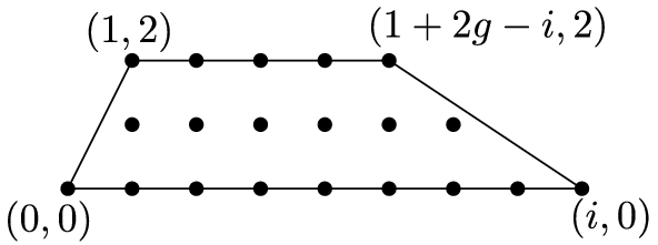
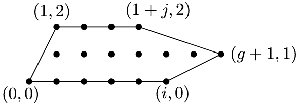
For $g=2h$ even, set P to be the rectangle $\text {conv}\left( (0,0),(0,3),(h+1,0),(h+1,3)\right)$; for $g=2h+1$ odd, set P to be the trapezoid $\text {conv}\left( (0,0),(0,3),(h+3,0),(h,3)\right)$. We claim that the polygon P has genus g, and $\dim (\mathbb {M}_P)=2g+1$ for $g>3$ and $\dim (\mathbb {M}_P)=2g$ for $g=3$; this was proved in [2, Theorem 1.1]. Define Q to be a subpolygon of P with the same interior polygon, in the even case as $\text {conv}\left( (1,0),(0,3),(h+1,1),(h+1,2)\right)$ and in the odd case as $\text {conv}\left( (1,0),(0,3),(h+2,1),(h+1,2)\right)$. These polygons P and Q for the even and odd cases are illustrated in Fig. 13. Because Q only has 4 boundary points (all vertices), an optimal triangulation will only yield moduli dimension $g+1$ by Proposition 3. Thus, we have $\dim (\mathbb {M}_Q)=g+1$. Consider a sequence of convex lattice polygons $P=P_0\supsetneq P_1\supsetneq P_2\supsetneq \cdots \supsetneq P_k=Q$, where $P_i$ has exactly one more lattice point than $P_{i+1}$. Since $P_\text {int}=Q_\text {int}$, all these polygons have genus g. By [6, §5], if $P''\subset P'$ and $P'$ has exactly one more lattice point than $P''$, then $\dim (\mathbb {M}_{P'})-1\le \dim (\mathbb {M}_{P''})\le \dim (\mathbb {M}_{P'})$. In other words, moduli dimension can drop by at most one if we remove a single lattice point. Letting $a_i=\dim (P_i)$, we thus have $a_0=2g+1$, $a_k=g+1$, and $a_{i}-1\le a_{i+1}\le a_i$. It follows that the set of numbers $\{a_0,a_1,\ldots ,a_k\}$ must contain every integer from between $g+1$ and $2g+1$. In other words, every integer between $g+1$ and $2g+1$ must be equal to $\dim (\mathbb {M}_{P_i})$ for some i.

Fig. 13

The polygon P on the left and Q on the right, in the even case (top) and the odd case (bottom)

We now have that all values of d between $g+1$ and $2g+1$ are achieved as the moduli dimension of some polygon of genus g; the same is true for $d=g$ when $g\notin \{4,7\}$ by Proposition 4. This gives us all values of d with $\ell (g)\le d\le u(g)$ when $g\ne 7$. For $g=7$, we also need a polygon achieving the moduli dimension $2g+2$; this is furnished by the polygon $H_{4,4,2,6}$ in [2, Theorem 1.1], completing the proof.

$\square$

The fact that every intermediate moduli dimension between the upper and lower bounds is achieved is not something we can take for granted. For instance, if we restrict our attention to maximal non-hyperelliptic polygons, it is no longer the case that all intermediate values are achieved as a moduli dimension. Recall that a lattice polygon is called maximal if it is not properly contained in any lattice polygon of the same genus. These polygons are particularly interesting from the perspective of tropical geometry. As shown in [2, Lemma 2.4], if $P\subseteq Q$ where $P$ and $Q$ have the same number of interior lattice points, then $\mathbb {M}_P\subseteq \mathbb {M}_Q$. (This does not hold for $\mathcal {M}_P$ and $\mathcal {M}_Q$, as discussed in [4, §11].) It follows that the moduli space of all tropical plane curves $\mathbb {M}_g^{\text {planar}}$ can be decomposed as

$$\begin{aligned} \mathbb {M}_g^{\text {planar}}=\left( \bigcup _P \mathbb {M}_P\right) \cup \mathbb {M}_{T_g}, \end{aligned}$$

where the main union is taken over all maximal non-hyperelliptic lattice polygons of genus $g$, and where $T_g=\text {conv}((0,0),(0,2),(2g+2,0))$ is the standard hyperelliptic triangle of genus $g$.

Proposition 5

Let $g\ge 20$. If g is even, there does not exist any maximal non-hyperelliptic polygon of moduli dimension $2g-1$. If g is odd, there does not exist any maximal non-hyperelliptic polygon of dimension 2g.

Proof

The key polygons P of genus g in this proof will be those whose interior polygon $P_\text {int}$ has genus $g^{(1)}=0$. For $g\ge 7$, we know by [9, Theorem 4.1.2] that $P_\text {int}$ is equivalent to a trapezoid⁴$T_{a,b}$ with vertices at (0, 0), (0, 1), (b, 0), and (a, 1) where $0\le a\le b$ and $b\ge 1$. By [11, Proposition 4.1], $T_{a,b}$ is an interior polygon if and only if $a\ge \frac{1}{2}b-1$, or equivalently $a\ge \frac{g-2}{3}$. For such a $T_{a,b}$, the vertices of $T_{a,b}^{(-1)}$ are $(-1,-1)$, $(-1,2)$, $(2b-a+1,-1)$, and $(2a+1-b,2)$.

Let us compute the moduli dimension of $T_{a,b}^{(-1)}$. By [6, Lemma 3.7], to do this we may connect the interior vertices to their corresponding boundary vertices, add in the boundary of the interior polygon, and produce a “zigzag” pattern on the resulting width-1 polygons. For the interior points at height 0, this yields two points of Type 3 and $b-2$ points of Type 2 (contributing $b-2+2\cdot 2=b+2$ to $b_2+2b_3$). Before implementing the zigzag pattern for the top strip, there are two points (the interior vertices) at height 1 already of Type 2. Each lattice point at height 2 beyond (0, 0) allows us to promote one point at that height by one type, increasing $b_2+2b_3$ by one, until we get to the point that every interior point has been maximized as Type 3 for a vertex or Type 2 otherwise (yielding $b_2+2b_3=g-4+2\cdot 4=g+4$). There are $2a-b+2$ lattice points at height 2, so the final value of $b_2+2b_3$ is

$$\begin{aligned}\min \{g+4,b+2+2a-b+1\}=\min \{g+4,2a+3\}.\end{aligned}$$

This yields a moduli dimension of

$$\begin{aligned}\min \{2g+1,g+2a+2\}.\end{aligned}$$

Recalling that $\frac{g-2}{3}\le a\le \frac{g}{2}$, the only value of a for which the minimum is $2g+1$ is $a=\left\lfloor \frac{g}{2}\right\rfloor$. For $a=\left\lfloor \frac{g}{2}\right\rfloor -1$, the moduli dimension is $g+2a+3=g+2\left\lfloor \frac{g}{2}\right\rfloor$, which equals 2g for g even and $2g-1$ for g odd. Decreasing a from here causes the moduli dimension to drop by 2 at a time, until reaching $g+\left\lceil \frac{g-2}{3}\right\rceil +2$. In particular, for g even, none of these polygons have moduli dimension $2g-1$, and for g odd none have moduli dimension 2g.

It remains to show that no other maximal non-hyperelliptic polygon has moduli dimension $2g-1$ or 2g. Any other such polygon has $g^{(1)}\ge 1$. Let $r^{(1)}$ denote the number of interior boundary points, so that $g=r^{(1)}+g^{(1)}$. By the main theorem of [13], we know that the number of boundary points of a convex lattice polygon of positive genus is at most twice its genus plus seven, so $r^{(1)}\le 2g^{(1)}+7$. Thus, $g=r^{(1)}+g^{(1)}\le 3g^{(1)}+7$, which implies $g^{(1)}\ge (g-7)/3$. Since we’ve assumed $g\ge 20$, we have $g^{(1)}\ge (20-7)/3>4$, so $g^{(1)}\ge 5$. By [4, Corollary 10.6], we have that $\dim (\mathcal {M}_P)\le 2g+3-g^{(1)}$ for any maximal non-hyperelliptic polygon P. This also serves as an upper bound on $\dim (\mathbb {M}_P)$. Since $g^{(1)}\ge 5$, we have $\dim (\mathbb {M}_P)\le 2g+3-5=2g-2$. Thus, no maximal non-hyperelliptic polygon with $g^{(1)}\ge 1$ and $g\ge 20$ has moduli dimension $2g-1$ or 2g. This completes the proof. $\square$

Further investigation into the achievable moduli dimensions of maximal non-hyperelliptic polygons would be an interesting direction for future research.

4 Moduli dimensions of hyperelliptic polygons

We now move on to the case of hyperelliptic polygons, which have all interior lattice points collinear. These are somewhat simpler to describe than non-hyperelliptic polygons, and in fact a complete classification of hyperelliptic polygons of genus $g\ge 2$ was carried out in [9] and is also presented in [3]. We recall that result here.

Theorem 6

( [9]) If P is a hyperelliptic polygon of genus $g\ge 2$, then it is equivalent to precisely one of the following polygons, sorted into three classes.

• 1. Class 1:

  

  where $g \le i \le 2g$

• 2. Class 2:

  

  where (a) $0 \le i \le g$ and $0 \le j \le i$; or (b) $g < i \le 2g+1$ and $0 \le j \le 2g-i + 1$

• 3. Class 3:

  

  where (a) $0 \le k \le g+1$ and $0 \le i \le g+1-k$ and $0 \le j \le i$; or (b) $0 \le k \le g+1$ and $g+1-k < i \le 2g+2-2k$ and $0 \le j \le 2g -i- 2k + 1$

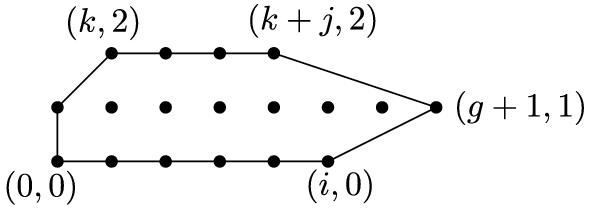
If we are considering a hyperelliptic polygon in one of these forms, each of its lattice points is of the form $(a,b)$ where $0\le b\le 2$. We refer to the value of $b$ as the height of the lattice point $(a,b)$. We also differentiate between several of the interior lattice points of such a polygon $P$. The two lattice points $(1,1)$ and $(g,1)$ are called the end interior points, with all other interior lattice points called middle interior points.

Fig. 14

Unimodular triangulations of a hyperelliptic lattice polygon; tropical curves dual to those triangulations; and the corresponding skeletons

Things are also simpler on the side of the tropical plane curves that have hyperelliptic Newton polygons. Three unimodular triangulations of a hyperelliptic polygon are illustrated in the left of Fig. 14, followed by tropical curves dual to those triangulations, followed by the skeletons of those curves. As with any smooth tropical plane curve $\varGamma$, there will be a bounded region of $\mathbb {R}^2\setminus \varGamma$ for each interior lattice point of the Newton polygon $P$; the skeleton can be thought of as encoding how these bounded regions sit relative to one another. Due to the collinearity of the interior lattice points of a hyperelliptic polygon $P$, there is a natural left-to-right ordering on these faces; the only possible relationships between the $i^{th}$ face and the $(i+1)^{th}$ face are that they either share a common edge (when the corresponding interior lattice points of $P$ are joined by an edge in the triangulation), or are separated by a bridge (otherwise). The upshot of this is that the skeleton of a smooth tropical curve with hyperelliptic Newton polygon is always a particular type of graph called a chain [2, §6].

We define a chain of genus g to be any trivalent graph that arises from the following construction. Start with a path graph with $g-1$ vertices. Duplicate each edge to a bi-edge and attach two loops to the two endpoints. This gives us a 4-regular graph. For each 4-valent node, we resolve it into two 3-valent nodes in one of two ways, one giving a shared edge between two bounded faces and one giving a bridge connecting two bounded faces. The starting 4-regular graph, the two allowed resolutions for each node, and the resulting chains for genus 3 are illustrated in Fig. 15. Note that these are precisely the skeletons that appeared in Fig. 14.

Fig. 15

The starting 4-regular graph, the two resolution choices, and the resulting trivalent chains of genus 3

We set the following labeling convention for the edge lengths of a chain, as illustrated in Fig. 16. We will assume that our chain has come from an embedding of a tropical curve, and so has a well-defined orientation of its bounded faces from left to right. The leftmost edge length is called e, and the rightmost f. For the $i^{th}$ bounded face where $2\le i\le g-1$, we let $u_i$ (respectively $\ell _i$) denote the length of the upper (respectively lower) edge bounding that face. Finally, if the $i^{th}$ and $(i+1)^{th}$ faces are separated by a bridge, call its length $b_{i,i+1}$ (and by convention set $h_{i,i+1}=0$), and if they instead share an edge, call its length $h_{i,i+1}$ (and by convention set $b_{i,i+1}=0$).

Fig. 16

The edge length labels for a chain

Given a unimodular triangulation $\mathcal {T}$ of a hyperelliptic Newton polygon P, we wish to consider the constraints on the edge lengths of a skeleton $\varGamma$ of a dual tropical curve. There are a few immediate constraints (or lack thereof) on the edge lengths of $\varGamma$. First, all edge lengths must be positive (or nonnegative, after we take closures). Second, we have $u_i=\ell _i$ for all i by [10, Lemma 2.2]. Third, there are no restrictions on any nonzero $b_{i,i+1}$’s; this is a general property of bridges in tropical plane curves. Similarly, if e (or f) is the length of a loop incident to a bridge, then there are no restrictions on it. The further inequalities are more subtle and depend on the structure of the triangulation $\mathcal {T}$. We will first handle those coming from the $2^{nd}$ through $(g-1)^{th}$ faces and then those pertaining to the extremal edges $e$ and $f$.

Without loss of generality, we assume that P is of a form from Theorem 6, with interior lattice points at (i, 1) for $1\le i\le g$. For each i, let NW(i) denote the x-coordinate of the leftmost lattice point at height 2 connected to (i, 1); NE(i) that of the rightmost such point at height 2; and similarly for SW(i) and SE(i) at height 0. These labels are illustrated in Fig. 17, along with the corresponding cycle from the tropical curve; the edges are considered as vectors, with labels that will be useful in our next proof. Note that the non-vertical edges of a cycle all have integral slope, due to the slopes of the edges in $\mathcal {T}$.

Fig. 17

Edges connecting $(i,1)$ to boundary points at heights $0$ and $2$ and the cycle corresponding to $(i,1)$, with edges considered as vectors

Lemma 3

Suppose $2\le i\le g-1$. The only additional constraint involving $u_i$ is

$$\begin{aligned}(2i-NW(i)-SW(i))u_i\le h_{i,i+1}-h_{i-1,i} \le (2i-NE(i)-SE(i))u_i,\end{aligned}$$

with equality if and only if the tropical curve contributes only one edge to the upper and lower edges of the $i^{th}$ face.

This was originally proven in [12, §3.6]; we include our own proof for completeness.

Proof

Order the edges of $\varGamma$ contributing to the $i^{th}$ face clockwise as vectors, say as $\overline{v}_1,\overline{w}_1,\ldots ,\overline{w}_m, \overline{v}_2,\overline{x}_1,\ldots ,\overline{x}_{n}$ where $\overline{v}_1=\left<0,h_{i-1,i}\right>$, where $\overline{v}_2=\left<0,-h_{i,i+1}\right>$, where $\overline{w}_1,\ldots ,\overline{w}_m$ form the upper edge in the skeleton, and where $\overline{x}_1,\ldots ,\overline{x}_{n}$ form the lower edge in the skeleton. An example of this labeling scheme appears on the right in Fig. 17. Note that it is possible for $v_1$ or $v_2$ to be the zero vector, but all other vectors are nonzero.

These vectors form a closed cycle if and only if

$$\begin{aligned}\overline{v}_1+\overline{w}_1+\cdots +\overline{w}_m+\overline{v}_2+\overline{x}_1+\cdots +\overline{x}_{n}=\left<0,0\right>,\end{aligned}$$

which can be rearranged to

$$\begin{aligned}-\overline{v}_1-\overline{v}_2=\overline{w}_1+\cdots +\overline{w}_m+\overline{x}_1+\cdots +\overline{x}_{n}.\end{aligned}$$

The first vector is $\left<0,h_{i,i+1}-h_{i-1,i}\right>$. Now, let $\widehat{w}_j$ be the primitive integer vector with the same direction of $\overline{w}_j$, so that $\overline{w}_j=\ell (\overline{w}_j)\widehat{w}_j$ with $\ell$ denoting lattice length; set the same notation for $\widehat{x}_j$. Considering the possible slopes of the edges in $\mathcal {T}$ that $\overline{w}_j$ are dual to, we have that $\hat{w}_j=\left<1,r_j\right>$ for some integer $r_j$, and similarly we $\hat{x}_j=\left<-1,s_j\right>$ for some integer $s_j$. Our vector sum thus gives us

$$\begin{aligned}0=\ell (\overline{w}_1)+\cdots +\ell (\overline{w}_m)-\ell (\overline{x}_1)-\cdots -\ell (\overline{x}_{n})\end{aligned}$$

from the first component, and

$$\begin{aligned}h_{i,i+1}-h_{i-1,i}=\ell (\overline{w}_1)r_1+\cdots +\ell (\overline{w}_m)r_m+\ell (\overline{x}_1)s_1+\cdots +\ell (\overline{x}_{n})s_n\end{aligned}$$

from the second. The first sum is equivalent to stating that the upper and lower edges of the $i^{th}$ face of $\varGamma$ must be equal in length, which we already knew. For the second sum, we first remark that $r_1>r_2>\ldots >r_m$, since these are the slopes of a convex-down sequence of edges; and similarly that $s_1<s_2<\ldots <s_n$. Replacing each $r_j$ with $r_1$ and each $s_j$ with $s_n$, we obtain the upper bound

$$\begin{aligned}h_{i,i+1}\!-\!h_{i-1,i}\le \ell (\overline{w}_1)r_1\!+\!\cdots \!+\!\ell (\overline{w}_m)r_1\!+\!\ell (\overline{x}_1)s_n\!+\!\cdots \!+\!\ell (\overline{x}_{n})s_n\!=\!(r_1\!+\!s_n)u_i,\end{aligned}$$

where we have equality if and only if no term was decreased, i.e., if $m=n=1$. Similarly, we find the lower bound

$$\begin{aligned}h_{i,i+1}\!-\!h_{i-1,i}\ge \ell (\overline{w}_1)r_m\!+\!\cdots \!+\!\ell (\overline{w}_m)r_m\!+\!\ell (\overline{x}_1)s_1\!+\!\cdots \!+\!\ell (\overline{x}_{n})s_1\!=\!(r_m\!+\!s_1)u_i,\end{aligned}$$

with equality if and only if $m=n=1$.

Note that the vector $\left<1,r_1\right>$ is perpendicular to the edge connecting $(i,1)$ to the leftmost point at height $2$, namely $(NW(i),2)$. It follows that $r_1=i-NW(i)$. Similarly, we have $r_m=i-NE(i)$. An identical argument shows that $s_1=SE(i)-i$ and $s_n=SW(i)-i$. Plugging these in to our upper bound of $(r_1+s_n)u_i$ and lower bound of $(r_m+s_1)u_i$ gives us the claimed bounds of

$$\begin{aligned}(2i-NW(i)-SW(i))u_i\le h_{i,i+1}-h_{i-1,i} \le (2i-NE(i)-SE(i))u_i.\end{aligned}$$

To ensure that there are no additional constraints, we need to show that for fixed $u_i$, we can achieve any value of $h_{i,i+1}-h_{i-1,i}$ in the interior of this range. We can find $h_{i,i+1}-h_{i-1,i}$ arbitrarily close to $(2i-NE(i)-SE(i))u_i$ by choosing $\ell (\overline{w}_1)$ and $\ell (\overline{x}_n)$ with lattice lengths $u_i-\varepsilon$ for a very small choice of epsilon, and distributing the remaining $\varepsilon$ of lattice length in any way among the remaining edges. An identical argument where most lattice length is given to $\ell (\overline{w}_m)$ and $\ell (\overline{x}_1)$ gets us $h_{i,i+1}-h_{i-1,i}$ arbitrarily close to $2i-NW(i)-SW(i))u_i$, completing the proof. $\square$

Having dealt with the constraints for the $i^{th}$ cycle where $2\le i\le g-1$, we now consider the edge e. For simplicity, we will assume that no edge in $\mathcal {T}$ connects the boundary to the boundary without cutting through the interior line segment; if there does exist such an edge, then we can iteratively pare off the triangles formed by such an edge and the boundary of P and obtain a triangulation $\mathcal {T}'$ of another hyperelliptic polygon $P'$ of the same genus, realizing the exact same metric graphs.

By Theorem 6, we know that the left end of a hyperelliptic polygon has one of two shapes, either Shape A (for Classes 1 and 2) or Shape $B_k$ (for Class 3). These shapes are illustrated in Fig. 18. We say that $\mathcal {T}$ has form A(m) with respect to e (resp. form $B_k(m)$ with respect to e) if the end has shape A (resp. $B_k$) and if (1, 1) is incident to exactly $m+1$ edges in $\mathcal {T}$: one connecting it to (2, 1), and m connecting it to boundary points.

Fig. 18

Two shapes of the left end of a hyperelliptic polygon

Lemma 4

Let $\mathcal {T}$ be a triangulation of a hyperelliptic polygon $P$ such that no edge in $\mathcal {T}$ connects the boundary to the boundary without cutting through the interior line segment. Let $e$ and $h_{1,2}$ be as in Fig. 16. If $e$ is a loop, there are no constraints on its length. Otherwise:

• (a) If $P$ has form $A(m)$ for $m\ge 3$, form $B_k(m)$ with $k\ge 2$, form $B_1(m)$ with $m\ge 4$, or form $B_0(m)$ with $m\ge 5$, then the only constraint on $e$ is $e\ge h_{1,2}$.

• (b) If $P$ has form $A(2)$, then $e=2h_{1,2}$.

• (c) If $P$ has form $B_0(3)$, then $e=h_{1,2}$.

• (d) If $P$ has form $B_0(4)$ or form $B_1(3)$, then the only constraint on $e$ is $h_{1,2}\le e\le 2h_{1,2}$.

Moreover, these cases are exhaustive.

Proof

By our assumption on $\mathcal {T}$, for Shape A we know e is connected to at least (0, 0) and (1, 2), and for Shape $B_k$ to (0, 0), (0, 1), and (k, 2); thus, for shape A we have $m\ge 2$, and for shape $B_k$ we have $m\ge 3$, meaning our cases listed are exhaustive.

Fig. 19

Several forms

First assume that P has shape A. Several forms of the triangulation $\mathcal {T}$ appear in Fig. 19, along with the face dual to (1, 1) in a tropical curve. Note that Form A(2) can appear in one way, while form A(3) can appear in two ways. First assume $m\ge 3$. The claimed constraint $e\ge h_{1,2}$ is certainly a necessary condition, in order for the first cycle to close up; to see that it is sufficient, we note that for form A(3) and beyond there are at least two parallel edges appearing in the face dual to (1, 1) (either horizontal or with slope 1) that are part of the edge e, allowing unlimited scaling. When $m=2$, we can see that $e=2h_{1,2}$ from the triangular structure of the cycle dual to $(1,1)$.

Fig. 20

Several forms of hyperelliptic triangulations

Now assume that P has shape $B_k$. We illustrate several possible forms for $0\le k\le 2$ in Fig. 20. For many cases ($B_k(m)$ with $k\ge 2$, as well as for $B_1(m)$ with $m\ge 4$ and $B_0(m)$ with $m\ge 5$), the only constraint is $e\ge h_{1,2}$. Again, this holds because we are guaranteed parallel edges contributing to e, allowing for unlimited scaling. Our last claims are that for $B_0(3)$ we find $e=h_{1,2}$, and for $B_0(4)$ and $B_1(3)$ we find $h_{1,2}\le e\le 2h_{1,2}$. These again come from considering the illustrated cycles dual to (1, 1), and putting more or less length into components of the cycle dual to (1, 1). This completes the proof. $\square$

A priori we cannot use our shapes to study the rightmost edge f, since Theorem 6 differentiates between the left and right sides of the polygon. However, every right end is equivalent to a left end through a reflection and a shearing transformation of the form , meaning that we may indeed conclude that f satisfies the same constraints as e based on the shape of the polygon at the right end.

We are now ready to compute the moduli dimension of a unimodular triangulation of a hyperelliptic polygon.

Proposition 6

Let $\mathcal {T}$ be a unimodular triangulation of a hyperelliptic polygon P of genus $g \ge 2$. Let $b_e$ be the number of end interior points that are connected to another interior lattice point and boundary points that are all collinear. Let $b_m$ be the number of middle interior points connected to exactly 2 boundary lattice points. Then, we have

$$\begin{aligned} \dim (\mathbb {M}_\mathcal {T}) = 2g-1 - b_e - b_m \end{aligned}$$

Proof

To prove this, we will consider the requirements on our edge lengths. There are $3g-3$ edges in a connected trivalent graph of genus g. The conditions that $u_i=\ell _i$ for $2\le i\le g-1$ remove $g-2$ degrees of freedom, leaving us with at most $2g-1$ degrees of freedom.

We now ask if there are any other equalities that come out of the length constraints. For the edges on the $i^{th}$ face with $2\le i\le g-1$, by Lemma 3, the only possibility to have equalities forced are if the upper and lower bounds on $h_{i+1,i}-h_{i-1,i}$ are equal to one another; in this case, we lose another degree of freedom. This happens precisely when $NW(i)+SW(i)=NE(i)+SE(i)$. But since $NW(i)\le NE(i)$ and $SW(i)\le SE(i)$ this happens precisely when $NW(i)=NE(i)$ and $SW(i)=SE(i)$. This is equivalent to (i, 1) being connected to exactly one boundary point at height 0 and exactly one boundary point at height 2. This is the same as (i, 1) being connected to exactly two boundary points, since it must be connected to at least 2. Thus, we have $b_m$ more degrees of freedom lost.

Finally, we consider the edges e and f. By Lemma 4, we lose a degree of freedom in the cases that the form of $\mathcal {T}$ is either A(2) or $B_0(3)$. But these are precisely the forms where the corresponding interior end point is only connected to collinear boundary points. This completes the proof. $\square$

Now that we can compute the moduli dimension of a hyperelliptic triangulation, we can move toward finding the moduli dimension of a hyperelliptic polygon. Since every hyperelliptic polygon of genus $g\ge 2$ is equivalent to exactly one of the polygons from Theorem 6, it is enough to find the moduli dimension of each polygon in this classification.

Proposition 7

If P is a hyperelliptic polygon of genus g, then

$$\begin{aligned} \dim (\mathbb {M}_P) = {\left\{ \begin{array}{ll} 2g-1 &{}\text{ if } P \text{ is } \text{ in } \text{ Class } \text{1 } \\ \min (g+i+j,2g-1) &{}\text{ if } P \text{ is } \text{ in } \text{ Class } \text{2(a) }\\ 2g-1 &{}\text{ if } P \text{ is } \text{ in } \text{ Class } \text{2(b) }\\ \min (g+i+j+1,2g-1) &{}\text{ if } P \text{ is } \text{ in } \text{ Class } \text{3(a) } \text{ and } k \ne 0\\ \min (g+i+j,2g-1) &{}\text{ if } P \text{ is } \text{ in } \text{ Class } \text{3(a) } \text{ and } k = 0\\ \min (g+i+j+1,2g-1) &{}\text{ if } P \text{ is } \text{ in } \text{ Class } \text{3(b) }, \end{array}\right. } \end{aligned}$$

where i, j,  and k are as in the classification.

Proof

First assume that P is in Class 1, or in Class 2 with condition (b) satisfied. Start a triangulation of P as follows. Connect all interior points in a line segment and connect the point (1, 2) to all interior lattice points. Then for $1\le \ell \le g$, connect the interior lattice point $(\ell ,1)$ to the boundary points $(\ell -1,0)$ and $(\ell ,0)$; this is possible since $i\ge g$. The start of this triangulation is depicted in Fig. 21 for a Class 1 polygon. Complete this to a unimodular triangulation in any way; this is guaranteed to be regular by [14, Proposition 3.4], which states that any unimodular triangulation of a hyperelliptic polygon is regular. Note that both end interior points are connected to at least 3 not-all-collinear points, and all middle interior points are connected to two points at height 0. Thus for this triangulation, $d=e=0$, so $\dim (\mathbb {M}_P)\ge \dim (\mathbb {M}_\mathcal {T})=2g-1$. Since $\dim (\mathbb {M}_P)\le 2g-1$ for any hyperelliptic polygon of genus g, we conclude that $\dim (\mathbb {M}_P)=2g-1$, as claimed.

Fig. 21

The start of a triangulation of a polygon in Class 1

Now we assume that P is in Class 2 with condition (a) satisfied; that is, we assume $0\le i\le g$ and $0\le j\le i$. We wish to show that the moduli dimension is $\min (g+i+j,2g-1)$. We cannot do better than $2g-1$, since this is the dimension of the moduli space of all hyperelliptic curves. Let us argue that we cannot do better than $g+i+j$. First we remark that in any unimodular triangulation, we connect (1, 1) to (1, 2) and (0, 0), and we connect (g, 1) to $(g+1,1)$, $(1+j,2)$, and (i, 0). Thus, (g, 1) does not contribute to $b_e$; (1, 1) does not contribute to $b_e$ if and only if it is connected to at least two points at height 0 or 2; and a middle interior point does not contribute to $b_m$ if and only if it is connected to at least two points at height 0 or 2. Each time one of the relevant $g-1$ interior points is connected to at least two points at height 0 or 2, that uses up one of the edges on the horizontal faces of P. There are $i+j$ of these, so at most $\min \{g-1,i+j\}$ of them fail to contribute to $b_e+b_m$. Conversely, at least $g-1-\min \{g-1,i+j\}=\min \{0,g-i-j-1\}$ contribute to $b_e+b_m$. Thus for any triangulation $\mathcal {T}$ we have $\dim (\mathbb {M}_\mathcal {T})=2g-1-e-d\le 2g-1-\min \{0,g-i-j-1\}=\min \{2g-1,g+i+j\}$. Note that there does exist a triangulation $\mathcal {T}$ achieving this upper bound: for $1\le \ell \le i$, connect the lattice point $(\ell ,1)$ to $(\ell -1,0)$ and $(\ell ,1)$; and for $i+1\le \ell \le \min \{g-1,j+1\}$ connect $(\ell ,1)$ to $(\ell -i,2)$. We conclude that $\dim (\mathbb {M}_P)=\min \{2g-1,g+i+j\}$. Such a triangulation is illustrated in Fig. 22.

Fig. 22

The start of a triangulation of a polygon in Class 2(a)

Finally, we move on to Class 3; examples of the three cases we deal with appear in Fig. 23. In Class 3(a), we have $0 \le k \le g+1$ and $0 \le i \le g+1-k$ and $0 \le j \le i$. If $k \ne 0$, the end interior points never contribute to $b_e$, so the minimum we can achieve is $g+1$. By the same argument as Class 2(a), we end up getting the maximum possible dimension as $\min (g+1+i+j,2g-1)$. When $k = 0$, the left end interior point can contribute to $b_e$ like Class 2(a) so we end up with moduli dimension $\min (g+i+j,2g-1)$. For Class 3(b), we wish to show that the moduli dimension is $\min (g+1+i+j,2g-1)$. First, note that the left end interior point can contribute to $b_e$ if and only if $k = 0$. However, when this happens, $i > g+1$, giving us full dimension of $2g-1$. Note that $g + i + j + 1 > 2g-1$ in this case. The right end interior point can contribute to $b_e$ if and only if $(k+j,2), (g+1,1), (i,0)$ all lie on a line segment. If they are vertical or the line slopes downward, again $i \ge g+1$ and we have full dimension of $2g-1$. The only other case is if the line slopes upward or $k+j> g+1 >i$. Note that $i +k > g+1$, so $2g-i -2k + 1 < g - k$. Thus, $j < g - k$ and $j+k < g$. Thus, such a line is impossible. With both endpoints not contributing to a loss of degrees of freedom, this now follows the same logic as when $k \ne 0$ in Class 3(a).

Fig. 23

The starts of a triangulations for polygons in Class 3(a) with $k\ne 0$, Class 3(a) with $k=0$, and Class 3(b)

$\square$

We now have an easy proof of Theorem 3.

Proof

(Proof of Theorem 3) By Proposition 7 and the fact that $i,j\ge 0$, we have that $g\le \dim (\mathbb {M}_P)\le 2g-1$ for any hyperelliptic polygon P of genus g. Conversely, let $g\le d\le 2g-1$. There does indeed exist a hyperelliptic polygon of genus g with $\dim (\mathbb {M}_P)=d$; for instance, choose P to be in Class 2(a) with $j=0$ and $i=d-g$. $\square$

We close by considering the relationship between $\dim (\mathbb {M}_P)$ and $\dim (\mathcal {M}_P)$ for hyperelliptic $P$; recall that for non-hyperelliptic polygons these two numbers are known to be equal, which allowed us to deduce Corollary 2. First we note that when $P$ is hyperelliptic, we have by [4, Lemma 5.1] that $\mathcal {M}_P\subset \mathcal {M}_g^{\text {hyp}}$, where $\mathcal {M}_g^{\text {hyp}}$ is the moduli space of all hyperelliptic curves of genus $g$. This space has dimension $2g-1$, so $\dim (\mathcal {M}_P)\le \dim ( \mathcal {M}_g^{\text {hyp}})=2g-1$. If the (tropical) moduli dimension of a hyperelliptic polygon is equal to the top possible value of $2g-1$, then since $2g-1=\dim (\mathbb {M}_P)\le \dim (\mathcal {M}_P)\le 2g-1$, we can conclude that $\dim (\mathbb {M}_P)= \dim (\mathcal {M}_P)=2g-1$. Thus based on Proposition 7 we have $\dim (\mathbb {M}_P)= \dim (\mathcal {M}_P)=2g-1$ in all of the following cases:

• When $P$ is in Class 1 or Class 2(b).

• When $P$ is in Class 2(a) with $i+j\ge g-1$.

• When $P$ is in Class 3(a) with $k\ne 0$ and $i+j+1\ge g-1$.

• When $P$ is in Class 3(a) with $k=0$ and $i+j\ge g-1$.

• When $P$ is in Class 3(b) with $i+j+1\ge g-1$.

To our knowledge, there is no result determining the dimension of the algebraic moduli spaces $\mathcal {M}_P$ where $P$ is an arbitrary hyperelliptic polygon, so we cannot easily compare our tropical formulas to the algebraic case when $\dim (\mathbb {M}_P)< 2g-1$. We conjecture that $\dim (\mathbb {M}_P)=\dim (\mathcal {M}_P)$ for all hyperelliptic polygons $P$ and leave this as an interesting direction for a future project.

References

Brannetti, S.: Melo, Margarida, Viviani, Filippo: on the tropical Torelli map. Adv. Math. 227(3), 2546–2586 (2011)
Brodsky, S., Joswig, M., Morrison, R., Sturmfels, Bernd: Moduli of tropical plane curves. Res. Math. Sci. 2, 31 (2015)
Castryck, W.: Moving out the edges of a lattice polygon. Discrete Comput. Geom. 47(3), 496–518 (2012)
Castryck, W., Voight, J.: On nondegeneracy of curves. Algebra Number Theory 3(3), 255–281 (2009)
De Loera, J. A., Rambau, J., Santos, F.: Triangulations, volume 25 of Algorithms and Computation in Mathematics. Springer-Verlag, Berlin, Structures for algorithms and applications. (2010)
Desmond, C., Neelav, D., Sifan, J., Ralph, M., Andrew, S.: The moduli space of tropical curves with fixed Newton polygon. To appear in Adv. in Geom
Diane, M., Bernd, S.: Introduction to tropical geometry, volume 161 of Graduate Studies in Mathematics. American Mathematical Society, Providence, RI, (2015)
Georg, P.: Geometrisches zur Zahlenlehre. Sitzungsberichte des deutschen naturwissenschaftlich-medicinischen Vereines für Böhmen “Lotos” in Prag. (Neue Folge) 19, 311–319 (1899)
Koelman, R.: The number of moduli of families of curves on a toric surface. Katholieke Universiteit de Nijmegen (1991). (PhD thesis)
Morrison, R.: Tropical hyperelliptic curves in the plane. J. Algebraic Comb. (2020)
Morrison, R.: Convex lattice polygons with all lattice points visible. Discrete Math. 344(1), 112161 (2021)
Ralph Elliott, M.: Tropical and non-Archimedean curves. ProQuest LLC, Ann Arbor, MI, (2015). University of California, Berkeley (PhD thesis)
Scott, P.R.: On convex lattice polygons. Bull. Austral. Math. Soc. 15(3), 395–399 (1976)
Volker, K., Ziegler, G. M.: Counting lattice triangulations. In Surveys in combinatorics, 2003 (Bangor), volume 307 of London Math. Soc. Lecture Note Ser., pages 277–307. Cambridge Univ. Press, Cambridge, (2003)
Acknowledgements
This work was carried out as part of the 2020 SMALL REU and was supported by NSF Grants DMS-1659037 and DMS-2011743 and by Williams College. We thank two anonymous referees for very helpful suggestions and comments on an early version of this paper.
Funding
Supported by National Science Foundation Grants DMS-1659037 and DMS-2011743, and by Deutsche Forschungsgemeinschaft, Germany (SFB-TRR 195 “Symbolic Tools in Mathematics and their Application”)
Author information
Authors and Affiliations
Corresponding author
Ethics declarations
Conflict of interest
not applicable.
Availability of the code
Additional information
Publisher's Note
Springer Nature remains neutral with regard to jurisdictional claims in published maps and institutional affiliations.
This work was carried out as part of the 2020 SMALL REU, supported by National Science Foundation Grant DMS-1659037 and by Williams College. Ralph Morrison was supported by National Science Foundation Grant DMS-2011743. Ayush Kumar Tewari was supported by the Deutsche Forschungsgemeinschaft, Germany (SFB-TRR 195 “Symbolic Tools in Mathematics and their Application”).
Rights and permissions
About this article
Cite this article
Echavarria, M., Everett, M., Huang, S. et al. Moduli dimensions of lattice polygons. J Algebr Comb 55, 559–589 (2022). https://doi.org/10.1007/s10801-021-01062-6
Received:
Accepted:
Published:
Issue Date:
DOI: https://doi.org/10.1007/s10801-021-01062-6