
Abstract
This paper looks at the conditions under which a dynamic Laffer effect occurs. Using a basic model, we explain and reconcile selected findings in the literature. We numerically show that a lower tax rate on capital income is the best candidate for obtaining a dynamic Laffer effect—here defined as an improvement in the long-run budget balance of the government. Moreover, ignoring the stock of initial debt and changes in labor supply lead to an overestimation and underestimation of the effect, respectively. Finally, we show that when lower taxes on factor income are financed by higher taxes on consumption, there exists a wide array of combinations for which there is an improvement in both the long-run government budget balance and lifetime welfare. These combinations, however, differ in their implications for labor supply and immediate welfare effects.


Notes
Fullerton (1982), for example, uses a static framework to analyze the Laffer curve, while Ireland (1994) is one of the first to incorporate long-run effects related to the Laffer curve in a dynamic framework. Analyses that use dynamic frameworks to analyze this issue are also called dynamic scoring exercises.
The direct budget effect covers the direct impact of fiscal policy reforms on government revenues and expenditures, the growth rate effect covers the impact on government revenues and expenditures over time, and the discount rate effect aligns the changes in current and future government revenues and expenditures.
The different conditions under which a dynamic Laffer effect occurs in the literature will be discussed in Sect. 3.3.
\(U(t)\equiv \phi \log C(t)+\eta \log [1-L(t)]+\theta \log G(t)\) if \(\sigma =1\).
This specification allows for immediate adjustment of the price of bonds such that constant portfolio shares of physical capital and government bonds in equilibrium are guaranteed. Hence, the specification abstracts from transitional dynamics in portfolio shares associated with fixed-price bonds, see Turnovsky (2000b, p. 438).
In the derivations, we omit time indices for convenience of notation.
Substituting (1) and (9) into (7a) and subsequently taking the logarithm and time derivative of the resulting expression gives Eq. (13a). Substituting (3) into (11) and subsequently taking the logarithm and time derivative of the resulting expression gives Eq. (13b). Equation (13c) is obtained by dividing both sides of (12) by K and making use of the expression of the consumption-capital ratio. The latter can be obtained by substituting (3) into (11) and rearranging terms. Finally, substituting (2) into (7d) and rearranging terms gives Eq. (13d).
The web appendix to the paper discusses the effects of changes in fiscal policy instruments on the growth rate in more detail. If the equilibrium is indeterminate, which is not supported by the calibration in Sect. 4, the results in Eqs. (18a) and (18b) are the opposite, see also Itaya (2008). While an analysis of the conditions under which an equilibrium is indeterminate or determinate is beyond the scope of our analysis, we rather formally derive our equilibrium from a general framework (cf. Benhabib and Farmer 1994) and verify it is determinate than impose it when setting up the framework.
Hereby, we make use of the expression for initial private consumption \(\tilde{C}(0)=[(1-\omega _{G})\tilde{L}^{\beta }-(\tilde{\gamma }+\delta )]K(0)\), which follows from the relationship between the growth rate and labor supply associated with product market equilibrium, see (16b).
More specifically, a dynamic Laffer effect is more likely to occur in our model when the initial lump-sum transfer-to-output ratio T(0) / Y(0) is relatively high. Given that the consumption-to-output ratio in equilibrium can be given by \(\frac{\tilde{C}}{\tilde{Y}}=[(1-\omega _{G})\tilde{L}^{\beta }-(\tilde{\gamma }+\delta )]\tilde{L}^{-\beta }\), both statements imply the same.
See Table 2 for a list of the countries we consider.
All data used for the calibration can be found in the web appendix to the paper.
The method for calculating the implicit tax rates is based on Mendoza et al. (1994). We use the implicit tax rate related to the taxation of income and profits of firms for the implicit tax rate on capital income, and we neglect the taxation of capital stocks and the taxation of capital transfers.
The ratio of labor supply to total time is calculated by dividing the total hours work per year by 7300. The resulting ratios are close to the ones aimed for in the literature, see Mendoza and Tesar (2005, p. 190). Data on the growth rates and interest payments of the government are taken from the AMECO database.
Data on the private consumption-to-output ratio, the lump-sum transfer-to-output ratio, and total investment-to-output ratio are taken from the AMECO database, where we use social transfers defined as social transfers other than in kind, mainly consisting of social benefits in the form of cash. Data on tax revenues are taken from the European Commission (2008).
Capital expenditures of the government are captured by total investments.
The web appendix to the paper discusses additional robustness checks for the calibration of the model.
The results are for the EA (15) economy. Results for the other economies can be found in the web appendix to the paper.
Fig. 1 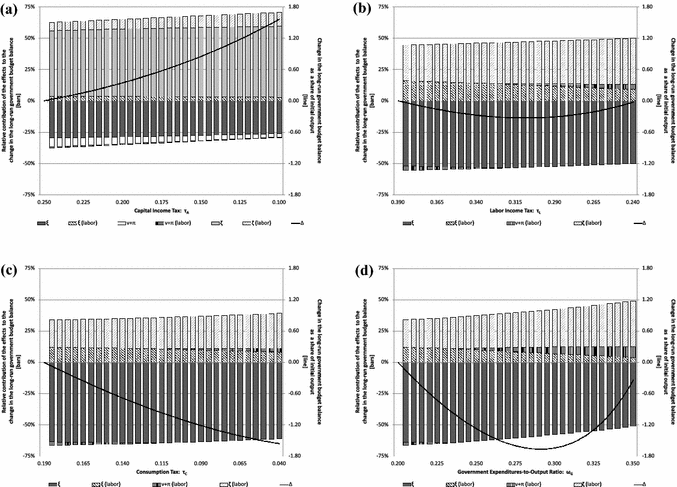
Effects of fiscal policy reforms for \(\tau _{A}, \tau _{L}, \tau _{C}\), and \(\omega _{G}\). Notes The relative contributions of the specific basic effects to the change in the long-rung government budget balance, given on the left vertical axis and represented by the bars, are obtained by diving the size of these basic effects by the sum of the absolute size of all basic effects. For example, for the direct budget effect it is given by \(\xi /\left( |\xi |+|\xi ^{l}|+|\nu |+|\nu ^{l}|+|\pi |+|\pi ^{l}|+|\zeta |+|\zeta ^{l}|\right) \). The change in the long-run government budget balance expressed as a share of initial output, given on the right vertical axis and represented by the line, is given by \((\xi +\xi ^{l}+\nu +\nu ^{l}+\pi +\pi ^{l}-\zeta -\zeta ^{l})/Y(0)\). a Capital income tax. b Labor income tax. c Consumption tax. d Government expenditures-to-output ratio
The graphs in Fig. 1 should not be compared to the traditional graphical representation of the Laffer curve that only applies to a single instrument. Our graphs look at the budget balance of the government in general so that even when a tax rate goes to zero, total government revenues not necessarily do so as well.
Note that the above- described effects are not the marginal effects as discussed in Sect. 3.2, but the effects are only related since we analyze discrete changes here. Notes on the specific method can be found in the web appendix to the paper.
Note that the direct budget effect of a change in a fiscal instrument does not correspond one-to-one with the initial size of the corresponding tax base since the tax base of other fiscal instruments also matters, see (21).
Technically, the direct budget effect can be negative as long as the combined discount rate effect and growth rate effect is positive. This situation is analyzed by Bruce and Turnovsky (1999) who argue that this situation is unlikely to occur in practice given the empirically implausible of the intertemporal elasticity of substitution it implies, see Sect. 3.3.
Notes on the method used are available in the web appendix to the paper.

References
Acemoglu, D. (2009). Introduction to modern economic growth. Princeton, NJ: Princeton University Press.
Agell, J., & Persson, M. (2001). On the analytics of the dynamic Laffer curve. Journal of Monetary Economics, 48, 397–414.
Attanasio, O. P., & Weber, G. (1993). Consumption growth, the interest rate and aggregation. Review of Economic Studies, 60, 631–649.
Barro, R. J., & Sala-i-Martin, X. (1999). Economic growth. Cambridge, MA: MIT Press.
Benhabib, J., & Farmer, R. E. A. (1994). Indeterminacy and increasing returns. Journal of Economic Theory, 63, 113–142.
Bruce, N., & Turnovsky, S. J. (1999). Budget balance, welfare, and the growth rate: ”Dynamic scoring” of the long-run government budget. Journal of Money, Credit and Banking, 31, 162–186.
European Commission. (2007). Statistical annex of European economy. Autumn 2007, Luxembourg.
European Commission. (2008). Taxation trends in the European Union. 2008 edition, Luxembourg.
Fernández, E., Pérez, R., & Ruiz, J. (2010). Double dividend, dynamic Laffer effects and public abatement. Economic Modelling, 27, 656–665.
Fredriksson, A. (2007). Compositional and dynamic Laffer effects in models with constant returns to scale. Research Papers in Economics 2007, Stockholm University, Department of Economics.
Fullerton, D. (1982). On the possibility of an inverse relationship between tax rates and government revenues. Journal of Public Economics, 19, 3–22.
Ireland, P. N. (1994). Supply-side economics and endogenous growth. Journal of Monetary Economics, 33, 559–571.
Itaya, Ji. (2008). Can environmental taxation stimulate growth? The role of indeterminacy in endogenous growth models with environmental externalities. Journal of Economic Dynamics and Control, 32, 1156–1180.
Laffer, A. B. (1979). Statement prepared for the joint economic committee, May 20. In A. Laffer & J. Seymour (Eds.), The economics of the tax revolt: A reader. New York: Harcourt Brace Jovanovich.
Leeper, E. M., & Yang, S. S. (2008). Dynamic scoring: Alternative financing schemes. Journal of Public Economics, 92, 159–182.
Mankiw, N. G., & Weinzierl, M. (2006). Dynamic scoring: A back-of-the-envelope guide. Journal of Public Economics, 90, 1415–1433.
Mendoza, E. G., & Tesar, L. L. (2005). Why hasn’t tax competition triggered a race to the bottom? Some quantitative lessons from the EU. Journal of Monetary Economics, 52, 163–204.
Mendoza, E. G., Razin, A., & Tesar, L. L. (1994). Effective tax rates in macroeconomics: Cross-country estimates of tax rates on factor incomes and consumption. Journal of Monetary Economics, 34, 297–323.
Novales, A., & Ruiz, J. (2002). Dynamic Laffer curves. Journal of Economic Dynamics and Control, 27, 181–206.
Strulik, H., & Trimborn, T. (2012). Laffer strikes again: Dynamic scoring of capital taxes. European Economic Review, 56, 1180–1199.
The Conference Board. (2009). Total economy database. June 2009. http://www.conference-board.org/economics
Trabandt, M., & Uhlig, H. (2011). The Laffer curve revisited. Journal of Monetary Economics, 58, 305–327.
Turnovsky, S. J. (2000a). Fiscal policy, elastic labor supply, and endogenous growth. Journal of Monetary Economics, 45, 185–210.
Turnovsky, S. J. (2000b). Methods of macroeconomic dynamics. Cambridge, MA: MIT Press.
Acknowledgments
This paper benefited from excellent comments and suggestions for improvement of two referees, and I would also like to thank Chul-In Lee, Jenny Ligthart, Harry Verbon, Stefania Villa, Simon Wehmüller, and seminar participants at Tilburg University, Georgia State University, the NAKE research day, the 66th IIPF Congress in Uppsala, the ENTER Jamboree, and the SMYE meeting for their feedback. All errors, however, remain my own.
Author information
Authors and Affiliations
Corresponding author
Additional information
This paper’s findings interpretations and conclusions are entirely those of the authors and do not necessarily represent the views of the World Bank, their Executive Directors, or the countries they represent.
Electronic supplementary material
Below is the link to the electronic supplementary material.
Appendix
Appendix
1.1 Existence of the equilibrium
Both (16a) and (16b) are defined for \(L\in (0,1]\). Over this interval, it holds that
where we used that \(0<\beta <1\). Moreover
Now, a unique equilibrium exists if \(\gamma _{P}(1)<\gamma _{Q}(1)\). This is the case if
1.2 Stability of the equilibrium
We define \(\varOmega _{P}(L)\equiv \partial \gamma _{P}(L)/\partial L\) and \(\varOmega _{Q}(L)\equiv \partial \gamma _{Q}(L)/\partial L\). The sign of the derivative of the rate of growth of labor supply (14) with respect to labor, valued at \(\tilde{L}\), is given by
If (28) is positive, then small deviations in labor supply lead to a permanent deviation from \(\tilde{L}\) so that the equilibrium is locally unstable and said to be locally determinate. If (28) is negative, then small deviations of the supply of labor will force labor supply back to \(\tilde{L}\) so that the equilibrium is locally stable and said to be locally indeterminate. Since \(\varOmega _{Q}(\tilde{L})>\varOmega _{P}(\tilde{L})\) when a unique equilibrium exists, and \(1-(1-\sigma )(\phi +\theta )>0\) by the concavity of the felicity function, the equilibrium is locally unstable if \(\varTheta ^{D}(\tilde{L})<0\).
1.3 Comparative static effects
The comparative static effects of the various tax rates are as follows:
where \(\varOmega _{P}(\tilde{L})>\varOmega _{Q}(\tilde{L})\) in the equilibrium that is determinate. In an indeterminate equilibrium, it holds that \(\varOmega _{P}(\tilde{L})<\varOmega _{Q}(\tilde{L})\) so that the effects are reversed.
Rights and permissions
About this article

Cite this article
van Oudheusden, P. Fiscal policy reforms and dynamic Laffer effects. Int Tax Public Finance 23, 490–521 (2016). https://doi.org/10.1007/s10797-015-9369-9
Published:
Issue Date:
DOI: https://doi.org/10.1007/s10797-015-9369-9