A Combined Weighting Based Large Scale Group Decision Making Framework for MOOC Group Recommendation

Abstract

Massive open online courses (MOOC) are free learning courses based on online platforms for higher education, which not only promote the open sharing of learning resources, but also lead to serious information overload. However, there are many courses on MOOCs, and it can be difficult for users to choose courses that match their individual or group preferences. Therefore, a combined weighting based large-scale group decision-making approach is proposed to implement MOOC group recommendations. First, based on the MOOC operation mode, we decompose the course content into three stages, namely pre-class, in-class, and post-class, and then the curriculum-arrangement-movement- performance evaluation framework is constructed. Second, the probabilistic linguistic criteria importance through intercriteria correlation method is employed to obtain the objective weighting of the criterion. Meanwhile, the word embedding model is utilized to vectorize online reviews, and the subjective weighting of the criteria are acquired by calculating the text similarity. The combined weighting then can be obtained by fusing the subjective and objective weighting. Based on this, the PL-MULTIMIIRA approach and Borda rule is employed to rank the alternatives for group recommendation, and an easy-to-use formula for group satisfaction is proposed to evaluate the effect of the proposed method. Furthermore, a case study is conducted to group recommendations for statistical MOOCs. Finally, the robustness and effectiveness of the proposed approach were verified through sensitivity analysis as well as comparative analysis.

1 Introduction

MOOC are a free online teaching pattern, characterized by a large-scale, open, and flexible organization, with course content covering a wide range of subjects from natural sciences to humanities (Alturkistani et al. 2020). MOOC successfully unlocked an advanced knowledge exchange whose main goal is to make resources from prestigious universities freely available to everyone, anywhere, with any device (Tseng et al. 2022). The three largest MOOC platforms in the world emerged in 2012 and were originally founded by professors at American universities (Macleod et al. 2016). Each platform offers hundreds of courses, has attracted millions of students, and has been reported as a new thing that is changing universities by Times (2012). Among them, edX only provides courses from top universities, Coursera is positioned to provide a platform that is available to any university, and Udacity mainly focuses on science and technology courses, especially computer science.

The first MOOC emerged from the open educational resources movement, and the number of MOOC learners has exceeded 300 million by 2021(Shah 2021). For example, Stanford offers free online college courses through their Office of the Vice Provost for Teaching and Learning (VPTL) in 1995; MIT announced program MITx in 2011, which offers massive open online courses in many disciplines. After the international MOOC storm, many renowned universities in China followed suite since 2012 (Doo et al. 2019; Wu 2021). For example, Peking University, Fudan University and Shanghai Jiao Tong University joined Coursera and edX MOOC platforms in 2013 respectively. Tsinghua University published MOOC platform “XuetangX” in 2013 (Li et al. 2021). In 2014, Shanghai Jiaotong University released “CNMOOC” and supported cross-campus learning and mutual recognition of credits in southwest China. By the end of 2021, more than 370 million registered students (MOE of China 2022) in China had studied online education platforms. MOOC have gradually matured and formalized, becoming one of the most popular online course development modes for higher education (Wu 2021). However, the emergence of diverse course resources has led to a serious information overload problem, which makes it tough for learners to choose the appropriate course because part of high-quality courses are concealed due to low clicks, while some low-quality courses are frequently recommended due to the high number of clicks. In addition, MOOC have been suffering from low course completion rates, ranging from 5 to 15% (Fidalgo-Blanco et al. 2016; Jordan 2015), which makes it difficult for learners to choose suitable MOOCs. Therefore, data analysis based on massive courses and recommending high-quality MOOCs to learners, thus solving the issues of painful class shopping and high trial-and-error costs, is an urgent task which remains to be solved in MOOC development.

Recommendation algorithms based on courses (online courses) mainly include: (1) content-based filtering approach (CBF). This approach mainly collects user and course attribute information, such as age, gender, text content, and number of clicks. Then algorithms such as TF-IDF are utilized to match user preferences with courses (Ghauth et al. 2010), thus implementing personalized recommendations for courses (Zhang et al. 2017); (2) collaborative filtering method (CF). The common practice is to model users based on association rules (Aher and Lobo 2013), KNN (Murad et al. 2020), social networks (Chen et al. 2022; Zhang et al. 2022; Zeng et al 2022), etc., to depict user portraits (Jing and Tang 2017), and then identify users with the same preference based on distance or similarity calculation methods, thus completing course recommendations; (3) machine learning-based recommendations. In this category, researchers mainly use machine learning methods to extract preference information of users (Hu et al. 2022) or courses (Xu and Zhou 2020), and employ Bayesian neural networks (Li et al. 2020), RNN (Okubo et al. 2017) to characterize the courses, and make course recommendation; (4) Hybrid-based recommendation. The primary objective of the hybrid recommendation models is to predicting students’ performance by combining the benefits of various recommendation methods and to recommend appropriate courses that match their interests by integrating personal information and course content (Esteban et al. 2019).

However, the following issues associated with recommendation methods and applications for courses (online courses) still exist:

• 1. Most existing methods recommend courses to individual users through personalized approaches. However, the audience of MOOC is dominated by college students, who mainly undertake learning activities as a group. Existing personalized course recommendation methods fail to satisfy the consistent preference demands of the group, resulting in inability to reach optimal group satisfaction in group decision making. Hence, group recommendations based on MOOC have emerged as an essential task.

• 2. In existing methods, the preference information of users is mainly represented by real numbers. However, the preference of each user is fuzzy and imprecise in real life because of cognitive bias, and they may be inconsistent and have different understanding towards the criteria when using MOOCs. Thus, users fail to deliver accurate evaluation information for each object. In addition, group preferences aggregated based on individual user preferences remain fuzzy and multidimensional, and real numbers fail to represent group preferences precisely. Thus, it is practical to conduct group recommendation research based on fuzzy information.

• 3. When multi-criterion recommendations are involved, methods such as AHP and entropy weighting are employed to estimate the criterion weights. However, these methods are either objective weights based on user preferences or subjective weights based on expert experience, and deviation exists in the recommendation results obtained by various weighting methods. Therefore, determining the appropriate weighting methods such that both subjective and objective information can be conveyed to achieve better recommendation results.

• 4. Most existing studies calculate criterion weights based on the user preference matrix. However, this method can only reflect the preferences of a single user or a part of them, which is limited. In fact, online reviews contain the preference information expressed by global users after completing the experience, which can reflect the real feelings of global users more intuitively. Therefore, the weights obtained by analyzing online reviews are more reasonable and referential.

Therefore, this study proposes a combined weighting based large-scale group decision-making (LSGDM) method for MOOC group recommendations.

The contributions of this research are as follows: (1) A large-scale group decision-making (LSGDM) method under probabilistic linguistic environment for online reviews is proposed. (2) Based on the MOOC operation mode, we decompose the course content into three stages, namely pre-class, in-class, and post-class, and then the Curriculum-Arrangement-Movement-Performance (CAMP) evaluation framework is constructed. (3) A combined weighting method is proposed in which the online review-based criterion subjective weighting with the users' preference-based objective weighting is integrated. (4) An easy-to-use formula for group satisfaction is proposed to evaluate the performance of group recommendations.

The architecture of the remaining parts of this study is organized as follows: The methodology of MCDM and the evaluation framework of MOOC is presented in Sect. 2. Then, Sect. 3 introduces the framework and steps of the proposed combined weighting based LSGDM method for group recommendation. Section 4 elaborates on the recommendation method through a specific case study. Finally, the conclusions and future work are summarized in Sect. 5.

2 Preliminaries

2.1 MOOC Quality Evaluation Criterion

Through literature review, a basic understanding of the MOOC operation pattern was obtained, and the specific process is shown in Fig. 1. From where it can be seen that the MOOC operation pattern mainly includes three phases: namely pre-class, in-class and post-class. Among them, the pre-class stage indicates that teachers release course resources through the online platform, so that students can preview the learning content and maximize the teaching effect. The in-class stage mainly focuses on students learning the knowledge of the lesson through the MOOC platform, discussing the questions detected in the pre-class phase, and displaying the learning results by completing class quizzes and online tests. The post-class stage mainly refers to the consolidation of the knowledge learned in the former two phases, while the teachers respond to the questions still encountered by students or release targeted learning tasks to make the MOOC learning pattern more accurate, comprehensive, and scientific.

Fig. 1

MOOC operation pattern

Considering the three stages of MOOC, a “CAMP” MOOC quality evaluation framework (see Table 1) is proposed, which contains four criteria, namely Curriculum, Arrangement, Movement, and Performance. Among them, Curriculum refer to the basic structure including course introduction, course framework, course outline, course objectives, faculty team, etc. Arrangement is a major part of the MOOC, which indicates the arrangement of the content of the MOOC including course videos, course resources, textbooks, reference materials, etc. Movement is organized to enhance the interaction and communication between teachers and students through learning forums, group discussions and homework, as well as to improve students' ability to implement independent learning and collaborative cooperation. Performance involves unit quizzes, midterm and final assessments, questionnaire feedback, etc., which is an assessment of the performance of the MOOC. Hence, the “CAMP” quality evaluation framework of MOOC is shown in Table 1.

Table 1 MOOC “CAMP” quality evaluation framework

2.2 Probabilistic Linguistic Term Sets

Decision makers typically utilize real numbers to evaluate online courses in MOOCs (Nie et al. 2020; Lu et al. 2017), but they fail to consider the fuzziness and unpredictability of user preferences. While the Probabilistic Linguistic Term Sets (PLTS) proposed by Pang et al. (2016) based on Linguistic Term Sets (LTS) can describe both hesitant and probabilistic components of uncertain information. In addition to expressing decision information in linguistic terms, decision makers can also reflect the preference degree through probability values, which can describe the real situation of decision makers more flexibly and appropriately than other fuzzy information (Zhang et al. 2018). Therefore, the concepts associated with the PLTS are introduced below.

Definition 1

Let $s_{t}$ be a linguistic term,$\tau$ is positive integer, $S = \{ s_{t} |t = - \tau , \ldots , - 1,0,1, \ldots ,\tau \}$ is a Linguistic Term Sets (LTS), which satisfies:

• (1) The $S$ is ordered: $s_{i} > s_{j}$ if $i > j$;

• (2) Negation operator: $Neg(s_{i} ) = s_{j}$, where $j = - i$;

• (3) Max operator: $\max \{ s_{i} ,s_{j} \} = s_{i}$, if $i \ge j$;

• 4) Min operator: $\max \{ s_{i} ,s_{j} \} = s_{j}$, if $i \le j$;

Definition 2

(Pang et al. 2016): It is assumed that $S = \{ s_{t} |t = - \tau , \ldots , - 1,0,1, \ldots ,\tau \}$ be a linguistic term set (LTS), then the definition of probabilistic linguistic term sets (PLTS) can be seen in Eq. (1):

$$ L(p) = \left\{ {L^{(k)} (p^{(k)} )|L^{(k)} \in S,r^{(k)} \in t,p^{(k)} \ge 0,k = 1, \ldots ,\# L(p),\sum\limits_{k = 1}^{\# L(p)} {p^{(k)} \le 1} } \right\}, $$

(1)

where $L^{(k)} (p^{(k)} )$ represents the linguistic term $L^{(k)}$ associated with the probability $p^{(k)}$, the number of distinct linguistic terms in $L(p)$ can be denoted as $\# L(p)$, $r^{(k)}$ is the subscript of linguistic terms. To be concise, $L^{(k)} (p^{(k)} )(k = 1,2, \ldots ,\# L(p))$ is a probabilistic linguistic element (PLE).

Definition 3

(Pang et al. 2016): Suppose $L_{1} (p)$ and $L_{2} (p)$ be any two PLTSs: $L_{1} (p) = \left\{ {L_{1}^{{(k_{1} )}} (p_{1}^{{(k_{1} )}} )|k = 1, \ldots ,\# L_{1} (p_{1} )} \right\}$ and $L_{2} (p) = \left\{ {L_{2}^{{(k_{2} )}} (p_{2}^{{(k_{2} )}} )|k = 1, \ldots ,\# L_{2} (p_{2} )} \right\}$. The generalized form of the Euclidean distance between $L_{1} (p)$ and $L_{2} (p)$ is shown in Eq. (2):

$$ d_{ned} (L_{1} (p),L_{2} (p)) = \left[ {\frac{1}{{\# L_{1} (p)}}\sum\limits_{k = 1}^{{\# L_{1} (p)}} {\left[ {d\left( {L_{1}^{{(k_{1} )}} (p_{1}^{{(k_{1} )}} ),L_{2}^{{(k_{2} )}} (p_{2}^{{(k_{2} )}} )} \right)^{2} } \right]} } \right]^{\frac{1}{2}} , $$

(2)

where $d(L_{1}^{{(k_{1} )}} (p_{1}^{{(k_{1} )}} ),L_{2}^{{(k_{2} )}} (p_{2}^{{(k_{2} )}} )) = \left| {p_{1}^{{k_{1} }} \times \frac{{r_{1}^{(k)} }}{\tau } - p_{2}^{{k_{2} }} \times \frac{{r_{2}^{(k)} }}{\tau }} \right|$, the number of linguistic terms in $L_{1} (p)$ and $L_{2} (p)$ can be represented as $\# L_{1} (p)$ and $\# L_{2} (p)$, which satisfied $\# L_{1} (p) = \# L_{2} (p)$.

Definition 4

(Luo et al. 2020): To measure the similarity between two PLTSs, the correlation coefficient of PLTS is proposed. It is assumed that $L_{1} (p)$ and $L_{2} (p)$ be any two PLTSs: $L_{1} (p) = \left\{ {L_{1}^{{(k_{1} )}} (p_{1}^{{(k_{1} )}} )|k = 1, \ldots ,\# L_{1} (p_{1} )} \right\}$ and $L_{2} (p) = \left\{ {L_{2}^{{(k_{2} )}} (p_{2}^{{(k_{2} )}} )|k = 1, \ldots ,\# L_{2} (p_{2} )} \right\}$, $\# L_{1} \left( p \right) = \# L_{2} \left( p \right)$, then Eq. (3) is utilized to calculate the correlation coefficient between $L_{1} (p)$ and $L_{2} (p)$:

$$ \kappa \left( {L_{1} \left( p \right),L_{2} \left( p \right)} \right) = \frac{{\left\langle {L_{1} \left( p \right),L_{2} \left( p \right)} \right\rangle }}{{\left| {L_{1} \left( p \right)} \right|\left| {L_{2} \left( p \right)} \right|}} = \frac{{\sum\nolimits_{k = 1}^{{\# L_{1} \left( p \right)}} {\left( {r_{1}^{(k)} p_{1}^{(k)} } \right)\left( {r_{2}^{(k)} p_{2}^{(k)} } \right)} }}{{\sqrt {\sum\nolimits_{k = 1}^{{\# L_{1} \left( p \right)}} {\left( {r_{1}^{(k)} p_{1}^{(k)} } \right)^{2} } } \sqrt {\sum\nolimits_{k = 1}^{{\# L_{1} \left( p \right)}} {\left( {r_{2}^{(k)} p_{2}^{(k)} } \right)^{2} } } }}. $$

(3)

Definition 5

(Pang et al. 2016): Assumed that $L(p) = \left\{ {L^{(k)} (p^{(k)} )|k = 1, \ldots ,\# L(p)} \right\}$ be a PLTS, then Eqs. (4) and (5) are conducted to calculate the score function $s\left( {L\left( p \right)} \right)$ and standard deviation $\sigma \left( {L(p)} \right)$ of PLTS $L\left( p \right)$:

$$ s\left( {L\left( p \right)} \right) = \sum\limits_{k = 1}^{\# L(p)} {g\left( {L^{\left( k \right)} } \right)p^{(k)} } /\sum\limits_{k = 1}^{\# L(p)} {p^{(k)} } , $$

(4)

$$ \sigma \left( {L(p)} \right) = \frac{{\left( {\sum\nolimits_{k = 1}^{\# L\left( p \right)} {\left( {g\left( {L^{\left( k \right)} } \right)p^{(k)} - s\left( {L\left( p \right)} \right)} \right)^{2} } } \right)^{1/2} }}{{\sum\nolimits_{k = 1}^{\# L\left( p \right)} {p^{(k)} } }}, $$

(5)

where $g\left( {L^{\left( k \right)} } \right) = \frac{{r^{(k)} + \tau }}{2\tau }$, $r^{(k)}$ is the subscript of linguistic term $L^{(k)}$.

After obtaining the probabilistic linguistic score function and standard deviation, the PLTSs can be compared. For example, given any two PLTSs $L_{1} (p)$ and $L_{2} (p)$:

• (1) if $s\left( {L_{1} \left( p \right)} \right) > s\left( {L_{2} \left( p \right)} \right)$, then $L_{1} (p) > L_{2} (p)$, and vice versa;

• (2) if $s\left( {L_{1} \left( p \right)} \right) = s\left( {L_{2} \left( p \right)} \right)$, then

• i. if $\sigma \left( {L_{1} (p)} \right) > \sigma \left( {L_{2} (p)} \right)$, then $L_{1} (p) > L_{2} (p)$, and vice versa;

• ii. if $\sigma \left( {L_{1} (p)} \right) = \sigma \left( {L_{2} (p)} \right)$, then $L_{1} (p)\sim L_{2} (p)$.

Definition 6

(Pang et al. 2016): Let $L_{i} \left( p \right) = \left\{ {s_{a,i}^{l} \left( {p_{i}^{l} } \right)\left| {l = 1,2, \ldots ,L_{i} } \right.} \right\}\left( {i = 1,2, \ldots ,n} \right)$ be $n$ PLTSs, $w^{T} = \left( {w_{1} ,w_{2} , \ldots ,w_{n} } \right)^{T}$ denotes the weighting vector, which satisfied $w_{j} \in \left[ {0,1} \right]$ and $\sum\nolimits_{j = 1}^{n} {w_{j} } = 1$. Then Eq. (6) is employed to calculate the probabilistic linguistic weighted averaging (PLWA) operator:

$$ \begin{aligned} & PLWA\left( {L_{1} \left( p \right),L_{2} \left( p \right), \ldots ,L_{m} \left( p \right)} \right) = w_{1} L_{1} \left( p \right) \oplus w_{2} L_{2} \left( p \right) \oplus \cdots \oplus w_{m} L_{m} \left( p \right) \\ &\quad = \cup_{{r_{1}^{n} \in L_{1} \left( p \right)}} \left\{ {w_{1} r_{1}^{n} p_{1}^{n} } \right\} \oplus \cup_{{r_{2}^{n} \in L_{2} \left( p \right)}} \left\{ {w_{2} r_{2}^{n} p_{2}^{n} } \right\} \oplus \cdots \oplus \cup_{{r_{m}^{n} \in L_{m} \left( p \right)}} \left\{ {w_{m} r_{m}^{n} p_{m}^{n} } \right\}, \\ \end{aligned} $$

(6)

when $w^{T} = \left( {{1 \mathord{\left/ {\vphantom {1 n}} \right. \kern-0pt} n},{1 \mathord{\left/ {\vphantom {1 n}} \right. \kern-0pt} n}, \ldots ,{1 \mathord{\left/ {\vphantom {1 n}} \right. \kern-0pt} n}} \right)^{T}$, the PLWA operator degenerates to the probabilistic linguistic averaging (PLA) operator.

2.3 PL-MULTIMOORA

The MULTIMOORA approach was first proposed by Brauers and Zavadskas (2010), which integrates the advantage of the additive utility function, multiplicative utility function as well as reference point method (Zhang et al. 2019; Zeng et al 2013). Li et al. (2020) extend the MULTIMOORA method in a probabilistic linguistic environment. Let $a_{i} \left( {i = 1,2, \ldots ,m} \right)$ be the alternatives, $c_{j} \left( {j = 1,2, \ldots ,n} \right)$ represent the criteria in the decision making progress, $L_{ij} \left( p \right)$ represent the decision maker’s probabilistic linguistic rating of alternative $a_{i}$ on criteria $c_{j}$. The following subsections describe probabilistic linguistic ratio system (PLRS), probabilistic linguistic reference point approach (PLRP) as well as probabilistic linguistic full multiplicative form (PLFMF) in the PL-MULTIMOORA approach:

2.3.1 Probabilistic Linguistic Ratio System (PLRS)

Let $s_{ij}$ be the score of $L_{ij} \left( p \right)$. Then Eq. (7) is employed to obtain the standardized normalized probabilistic linguistic score matrix $D\left( s \right) = \left( {s_{ij}^{N} } \right)_{n \times m}$:

$$ s_{ij}^{N} = \frac{{s_{ij} }}{{\sqrt {\sum\nolimits_{j = 1}^{m} {\left( {s_{ij} } \right)^{2} } } }}\left( {i = 1,2, \ldots ,n} \right), $$

(7)

Considering two types of criteria, which is benefit-based criteria as well as cost-based criteria. The Eq. (8) is utilized to calculate the utility value $U_{1} \left( {a_{i} } \right)\left( {i = 1,2, \ldots ,m} \right)$ in the PLRS system.

$$ U_{1} \left( {a_{i} } \right) = \sum\limits_{j = 1}^{g} {\omega_{j} } s_{ij}^{N} - \sum\limits_{j = g + 1}^{n} {\omega_{j} } s_{ij}^{N} , $$

(8)

where $c_{j} \left( {j = 1,2, \ldots ,g} \right)$ and $c_{j} \left( {j = g + 1,g + 2, \ldots ,n} \right)$ represent the benefit criterion and the cost criterion respectively. $\omega_{j}$ denotes the weight of $c_{j}$. The larger the value of $U_{1} \left( {a_{i} } \right)$, the higher the ranking of $a_{i}$.

2.3.2 Probabilistic Linguistic Reference Point Approach (PLRP)

The PLRP model is defined based on the linear normalization of PLE, which is expressed in Eq. (9):

$$ U_{2} \left( {a_{i} } \right) = \mathop {\max }\limits_{j} \omega_{j} \frac{{d\left( {s_{{ij^{ + } }} ,s_{ij} } \right)}}{{d\left( {s_{{ij^{ - } }} ,s_{{ij^{ + } }} } \right)}}, $$

(9)

where $s_{{ij^{ + } }}$ and $s_{{ij^{ - } }}$ denote the best and worst scores regarding to $c_{j}$, respectively. Therefore, the smaller the value of $U_{2} \left( {a_{i} } \right)$, the higher the ranking of alternative $a_{i}$.

2.3.3 Probabilistic Linguistic Full Multiplicative Form (PLFMF)

The PLRP guarantees that the performance of the chosen alternatives is not extremely poor under all criteria. According to Wu et al. (2018), the calculation process of PLFMF method is given by Eq. (10):

$$ U_{3} \left( {a_{i} } \right) = \frac{{\sqrt[g]{{\prod\nolimits_{j = 1}^{g} {\left( {1 - \left( {1 - s_{ij}^{N} } \right)^{{\omega_{j} }} } \right)} }}}}{{\sqrt[{n - g}]{{\prod\nolimits_{j = g + 1}^{n} {\left( {1 - \left( {1 - s_{ij}^{N} } \right)^{{\omega_{j} }} } \right)} }}}}, $$

(10)

where $U_{3} \left( {a_{i} } \right)$ is the utility value of $a_{i}$. The final alternative preference is obtained by sorting the $U_{3} \left( {a_{i} } \right)$, the larger the $U_{3} \left( {a_{i} } \right)$, the higher the ranking of $a_{i}$.

2.3.4 Borda Rule

Referring to Wu et al. (2018), an improved Borda rule was utilized to assess the Borda score by integrating the utility value obtained in the PLRS, PLRP, and PLFMF methods, which can be seen in Eqs. (11) and (12):

$$ U_{y}^{N} (a_{i} ) = \frac{{U_{y} (a_{i} )}}{{\sqrt {\sum\nolimits_{i = 1}^{m} {(U_{y} (a_{i} ))^{2} } } }},y = 1,2,3, $$

(11)

$$ IBS_{i} = U_{1}^{N} \left( {a_{i} } \right) \times \frac{{m - r_{1} \left( {a_{i} } \right) + 1}}{{{{m\left( {m + 1} \right)} \mathord{\left/ {\vphantom {{m\left( {m + 1} \right)} 2}} \right. \kern-0pt} 2}}} - U_{2}^{N} \left( {A_{i} } \right) \times \frac{{r_{2} \left( {a_{i} } \right)}}{{{{m\left( {m + 1} \right)} \mathord{\left/ {\vphantom {{m\left( {m + 1} \right)} 2}} \right. \kern-0pt} 2}}} + U_{3}^{N} \left( {A_{i} } \right) \times \frac{{m - r_{3} \left( {a_{i} } \right) + 1}}{{{{m\left( {m + 1} \right)} \mathord{\left/ {\vphantom {{m\left( {m + 1} \right)} 2}} \right. \kern-0pt} 2}}}, $$

(12)

where $IBS_{i}$ is the Borda score of alternative $a_{i} \left( {i = 1,2, \ldots ,m} \right)$, $y = 1,2,3$ refers to the PLRS, PLRP, and PLFMF methods, $U_{y} \left( {a_{i} } \right)$ refers to the utility value obtained through the three methods, $U_{y}^{N} \left( {a_{i} } \right)$ is the corresponding normalized utility value, $r_{y} \left( {a_{i} } \right)$ is the ranking results of three methods.

2.4 Word Embedding

Word embedding is a vital part of natural language processing (NLP) that converts human-understood textual information into vectorial forms that can be understood by machines. Common word-embedding models include One-Hot, GloVe (Global Vectors for Word Representation), and Word2vec (Lauren et al. 2018; Rezaeinia et al. 2018). GloVe is a word embedding model based on the word co-occurrence matrix proposed by Pennington et al. (2014). Compared with other models, the GloVe model makes better use of global contextual information, speeds up the training iteration, shortens the training cycle, and provides better training results (Sakketou and Ampazis 2020). The objective function of the GloVe model is listed in Eq. (13):

$$ J = \sum\limits_{i,j}^{N} {f\left( {X_{ij} } \right)\left( {v_{i}^{T} v_{j} + b_{i} + b_{j} - \log \left( {X_{ij} } \right)} \right)}^{2} , $$

(13)

where $v_{i}$ and $v_{j}$ are the word vectors for ${\text{word}}_{i}$ and ${\text{word}}_{j}$. $b_{i}$ and $b_{j}$ are the bias items of $v_{i}$ and $v_{j}$, respectively. $N$ is the size of the glossary; $f\left( {X_{ij} } \right)$ is the weighting function that dominates the frequency of co-occurrence word pairs; the higher the frequency, the greater the weight. Hence, the operation process of the GloVe model is:

2.5 PL-CRITIC

Criteria Importance through Intercriteria Correlation (CRITIC) is proposed to compute the objective weight of criterion (Diakoulaki et al. 1995), which involves calculating correlation coefficients and standard deviations of criteria and then determining the objective weights through both contrast strength and the conflicting nature of the indicators (Krishnan 2021). Wang et al. (2021) extended this approach to a probabilistic linguistic environment, which was calculated using Eqs. (14)–(17):

$$ w_{j} = \frac{{I_{j} }}{{\sum\nolimits_{j = 1}^{n} {I_{j} } }}, $$

(14)

$$ I_{j} = \sigma_{j} \sum\limits_{t = 1}^{n} {\left( {1 - \rho_{jt} } \right)} , $$

(15)

$$ \rho_{jt} = \frac{{\sum\nolimits_{i = 1}^{m} {\left( {\sum\nolimits_{k = 1}^{\# L\left( p \right)} {\left( {r_{ij}^{(k)} p_{ij}^{(k)} - \overline{r}_{j}^{(k)} \overline{p}_{j}^{(k)} } \right)} } \right)\left( {\sum\nolimits_{k = 1}^{\# L\left( p \right)} {\left( {r_{it}^{(k)} p_{it}^{(k)} - \overline{r}_{t}^{(k)} \overline{p}_{t}^{(k)} } \right)} } \right)} }}{{\sqrt {\sum\nolimits_{i = 1}^{m} {\left( {\sum\nolimits_{k = 1}^{\# L\left( p \right)} {\left( {r_{ij}^{(k)} p_{ij}^{(k)} - \overline{r}_{j}^{(k)} \overline{p}_{j}^{(k)} } \right)} } \right)^{2} } \sum\nolimits_{i = 1}^{m} {\left( {\sum\nolimits_{k = 1}^{\# L\left( p \right)} {\left( {r_{it}^{(k)} p_{it}^{(k)} - \overline{r}_{t}^{(k)} \overline{p}_{t}^{(k)} } \right)} } \right)^{2} } } }}, $$

(16)

$$ \sigma_{j} = \sqrt {\frac{1}{m}\sum\nolimits_{i = 1}^{m} {\left( {\sum\limits_{k = 1}^{\# L\left( p \right)} {\left( {r_{ij}^{(k)} p_{ij}^{(k)} - \overline{r}_{j}^{(k)} \overline{p}_{j}^{(k)} } \right)} } \right)^{2} } } , $$

(17)

where $w_{j}$ is the objective weight of criteria and satisfies $w_{j} \in \left[ {0,1} \right]$, $\sum\limits_{j = 1}^{n} {w_{j} = 1}$. $I_{j}$ is the amount of potential information possessed by criterion $c_{j}$.$\rho_{jt}$ is the correlation coefficient between criterion $c_{j}$ and $c_{t}$ based on Eq. (3), $\sigma_{j}$ is the standard deviation of the criterion $c_{j}$ according to Eq. (5), $\overline{r}_{j}^{(k)} \overline{p}_{j}^{(k)} = \frac{{\sum\nolimits_{i = 1}^{m} {r_{ij}^{(k)} } }}{m}\left( {\frac{{\sum\nolimits_{i = 1}^{m} {p_{ij}^{(k)} } }}{m}} \right)$.

3 The Combined Weighting Based LSGDM Model for Group Recommendation

3.1 The Framework of the Combined Weighting Based Group Recommendation Model

The LSGDM-based group recommendation model proposed in this paper consists of four modules: online review-based weighting process, clustering process, combined weighting process, ranking and recommendation process. The details are shown in Fig. 2.

• (1) Online review-based weighting process. The main contribution of this process is to crawl online reviews and extract text feature words based on NLP technology for text preprocessing. Then, the GloVe model is employed to vectorize the text feature words. Thus, the criterion weights can be obtained by calculating and normalizing the vector similarity between online reviews and criterion keywords.

• (2) Clustering process. This process aims to cluster user preferences using the K-means algorithm, so that users with the same preferences are gathered into the same sub-cluster, thus ensuring that the preferences of users within the subgroup are highly similar, while the preferences of users between subgroups differ.

• (3) Combined weighting process. The criterion weights obtained in this study were derived from two aspects: online review-based subjective weighting and user preference decision-making matrix-based objective weighting. The final criterion weights were obtained by fusing the two weights.

• (4) Ranking and recommendation processes. The alternatives were ranked using the PL-MULTIMOORA method, which consists of three parts: PLRS, PLRP, and PLFMF. Each part yields a utility value and ranking results for a set of alternatives. Furthermore, the Borda scores of the alternatives are calculated to determine the ultimate ranking in accordance with the Borda rule.

Fig. 2

Framework of the combined weighting based group recommendation model

3.2 The Steps of the Combined Weighting Based Group Recommendation Model

It is assumed that alternatives set is represented as $A = \left\{ {a_{1} ,a_{2} , \ldots ,a_{m} } \right\}$, $E = \left\{ {e_{1} ,e_{2} , \ldots ,e_{t} } \right\}$ be the users set, criterion set can be denoted as $C = \left\{ {c_{1} ,c_{2} , \ldots ,c_{n} } \right\}$, user weight vector $\Lambda = \left\{ {\lambda_{1} ,\lambda_{2} , \ldots ,\lambda_{t} } \right\}$ and criterion weight vector $\Omega = \left\{ {\omega_{1} ,\omega_{2} , \ldots ,\omega_{n} } \right\}$ remain unknown, but satisfy $\lambda_{k} \ge 0$ and $\sum\nolimits_{k = 1}^{t} {\lambda_{k} = 1}$, $\omega_{j} \ge 0$ and $\sum\nolimits_{j = 1}^{n} {\omega_{j} = 1}$. Then the probabilistic linguistic decision-making matrix $R_{ij}^{k}$ of user $e^{k}$ for the set of alternatives can be express using Eq. (18):

$$ R_{ij}^{k} = \left[ {\begin{array}{*{20}l} {L_{11}^{k} \left( p \right)} & {L_{12}^{k} \left( p \right)} & \cdots & {L_{1n}^{k} \left( p \right)} \\ {L_{21}^{k} \left( p \right)} & {L_{22}^{k} \left( p \right)} & \cdots & {L_{2n}^{k} \left( p \right)} \\ \vdots & \vdots & \ddots & \vdots \\ {L_{m1}^{k} \left( p \right)} & {L_{m2}^{k} \left( p \right)} & \cdots & {L_{mn}^{k} \left( p \right)} \\ \end{array} } \right], $$

(18)

where $L_{ij}^{k} \left( p \right)$ denotes the probabilistic linguistic rating of the user $e^{k}$ for $i{\text{th}}$ alternative with regard to criterion $c_{j}$. The pseudocode of the proposed combined weighting based LSGDM method for MOOC group recommendation is presented in Algorithm 2.

The proposed combined weighting based LSGDM method for MOOC group recommendation includes the following steps.

Step 1: Data acquisition and pre-processing. Based on Python web crawler technology, web data are parsed to obtain online reviews of users. Text feature words can then be accessed through NLP technology, including word segmentation, part-of-speech tagging, and stop-word removal.

Step 2: Building word vector. In accordance with Algorithm 1, the word co-occurrence matrix was obtained by setting a sliding window based on text feature words. The GloVe model is then utilized to train the text feature words to obtain the word vector according to Eq. (13).

Step 3: Calculate text similarity. After obtaining the word vector, the similarity of the word vector between the online reviews and criterion keyword words must be further calculated based on Eq. (19):

$$ \cos \left( {v_{i} ,v_{j} } \right) = \frac{{v_{i} \times v_{j} }}{{\left\| {v_{i} } \right\| \times \left\| {v_{j} } \right\|}}, $$

(19)

where $v_{i}$ and $v_{j}$ represent the word vectors of text feature words and $\cos \left( {v_{i} ,v_{j} } \right)$ denotes the similarity of word vectors.

Step 4: Calculate the online reviews-based criterion weighting. The online review-based criterion weights $q_{j}$ were obtained by normalizing the average similarity of the word vector, which was calculated using Eq. (20):

$$ q_{j} = \frac{{sim_{j} }}{{\sum\nolimits_{j = 1}^{n} {sim_{j} } }}, $$

(20)

where $sim_{j} = \sum\nolimits_{j = 1}^{n} {\cos \left( {v_{i} ,v_{j} } \right)}$ is the average similarity of word vectors for criterion $c_{j}$.

Step 5: User preference clustering. The probabilistic linguistic distances of each user’s rating regarding to alternative $a_{i}$ are calculated in accordance with Eqs. (1)–(2). Subsequently, the K-Means algorithm was used to cluster the users' preferences, and the clustering evaluation indexes, namely the Silhouette Coefficients (SC) index, Calinski-Harabaz (CH) Index, and Davies-Bouldin (DB) index, were calculated. The above process is repeated until all users are divided into $g$ subclusters, denoted as $G^{\left( 1 \right)} ,G^{\left( 2 \right)} , \ldots ,G^{\left( g \right)}$.

Step 6: Calculating the weights of users and subclusters. Based on ANOVA, the average standard deviation of each user's probabilistic linguistic rating was calculated using Eq. (5), and the weight $\lambda_{k}$ assigned to each user can be obtained by normalizing the average standard deviation as follows:

$$ \lambda^{k} = \frac{{\overline{\sigma }^{k} }}{{\sum\nolimits_{k = 1}^{t} {\overline{\sigma }^{k} } }}, $$

(21)

where $\overline{\sigma }^{k} = {{\sum\nolimits_{i = 1}^{m} {\sum\nolimits_{j = 1}^{n} {\sigma_{ij}^{k} } } } \mathord{\left/ {\vphantom {{\sum\nolimits_{i = 1}^{m} {\sum\nolimits_{j = 1}^{n} {\sigma_{ij}^{k} } } } {\left( {n \times m} \right)}}} \right. \kern-0pt} {\left( {n \times m} \right)}}$ denotes the average standard deviation of the probabilistic linguistic rating for each user. Then the user weights are summed to get the weights of subclusters $\lambda^{\left( r \right)} = \sum\nolimits_{k \in r} {\lambda^{k} }$.

Step 7: Construct the collective probabilistic linguistic decision matrix. Based on the PLWA operator, the probabilistic linguistic decision matrix $R^{\left( r \right)}$ for the sub-cluster is obtained by integrating the user weights $\lambda^{k}$ and user preference matrix $R_{ij}^{k}$.

$$ R^{\left( r \right)} = \left[ {\begin{array}{*{20}l} {L_{11}^{\left( r \right)} \left( p \right)} & {L_{12}^{\left( r \right)} \left( p \right)} & \cdots & {L_{1n}^{\left( r \right)} \left( p \right)} \\ {L_{21}^{\left( r \right)} \left( p \right)} & {L_{22}^{\left( r \right)} \left( p \right)} & \cdots & {L_{2n}^{\left( r \right)} \left( p \right)} \\ \vdots & \vdots & \ddots & \vdots \\ {L_{m1}^{\left( r \right)} \left( p \right)} & {L_{m2}^{\left( r \right)} \left( p \right)} & \cdots & {L_{mn}^{\left( r \right)} \left( p \right)} \\ \end{array} } \right]. $$

Similarly, the collective probabilistic linguistic decision matrix $R$ can be constructed by integrating the weights $\lambda^{\left( r \right)}$ and preference decision matrix $R^{\left( r \right)}$ of the sub-clusters.

$$ R = \left[ {\begin{array}{*{20}l} {L_{11} \left( p \right)} & {L_{12} \left( p \right)} & \cdots & {L_{1n} \left( p \right)} \\ {L_{21} \left( p \right)} & {L_{22} \left( p \right)} & \cdots & {L_{2n} \left( p \right)} \\ \vdots & \vdots & \ddots & \vdots \\ {L_{m1} \left( p \right)} & {L_{m2} \left( p \right)} & \cdots & {L_{mn} \left( p \right)} \\ \end{array} } \right], $$

where $L_{ij} \left( p \right)$ is the probabilistic linguistic rating of alternative $a_{i}$ under criterion $c_{j}$.

Step 8: Calculating combined weighting. In accordance with the collective probabilistic linguistic decision matrix, the objective weight of the criteria $w_{j}$ can be obtained according to Eqs. (14)–(17). Further, since the online review-based criterion weight $q_{j}$ is obtained in step (4), the combined weight of the criterion $\omega_{j}$ can be calculated using Eq. (22):

$$ \omega_{j} = \frac{{w_{j} \times q_{j} }}{{\sum\nolimits_{j = 1}^{n} {w_{j} \times q_{j} } }}. $$

(22)

Step 9: Ranking and Recommendation. Based on Eqs. (7)–(10), the PL-MULTIMOORA method is employed to calculate the utility values of the alternatives, and the Borda rule is utilized to rank the alternatives based on Eqs. (11)–(12). Finally, the Top-N alternatives are recommended to the group.

Step 10: Calculate the group satisfaction. To evaluate the performance of group recommendation model, a distance-based satisfaction function is proposed based on (Zhu et al. 2018) to evaluate the performance of group recommendation which is shown in Eq. (23).

$$ Sa = \mathop {\min }\limits_{r} \left\{ {{1 \mathord{\left/ {\vphantom {1 {\frac{1}{m}\sum\limits_{i = 1}^{m} {\sqrt {\sum\limits_{j = 1}^{n} {\left( {\omega_{j} s_{ij}^{\left( r \right)} - \omega_{j} s_{ij} } \right)^{2} } } } }}} \right. \kern-0pt} {\frac{1}{m}\sum\limits_{i = 1}^{m} {\sqrt {\sum\limits_{j = 1}^{n} {\left( {\omega_{j} s_{ij}^{\left( r \right)} - \omega_{j} s_{ij} } \right)^{2} } } } }}} \right\}, $$

(23)

where $s_{ij}^{\left( r \right)}$ is the score of the sub-cluster $G^{\left( r \right)}$,$s_{ij}$ denotes the collective score, and $\omega_{j}$ represents the criterion weight. $Sa$ refers to group satisfaction: the higher the $Sa$, the higher the satisfaction of the group.

A flowchart of the proposed LSGDM-based method for group recommendations is shown in Fig. 3.

Fig. 3

Flowchart of LSGDM-based group recommendation model

4 Case Study

4.1 Practical Problem Description

The continued impact of COVID-19 has led to a shift from traditional offline teaching patterns to online teaching patterns. Thus, online learning has become a trend. iCourse (https://www.icourse163.org/) is an online learning and education platform jointly released by Higher Education Press of China and NetEase. The main purpose of iCourse is to undertake the mission of the Ministry of Education’s National Quality Open Courses, offering high quality MOOC courses to the public (see Fig. 4).

Fig. 4

Statistics courses and user reviews on iCourse platform

For students majoring in statistics, statistics courses are generally conducted in class groups. However, more than 20 colleges and universities are releasing statistics courses on iCourses as of March 2022. Therefore, it is necessary to choose an appropriate statistics course among diverse MOOC.

In this context, a class containing 20 students decided to conduct collective learning of MOOC statistics and 8 statistics MOOCs with more than 1000 cumulative participants were selected on the iCourse platform (the selection process of 20 students and 8 statistics MOOCs are shown in Appendix 1): Henan University of Economics and Law (a₁), Zhejiang University of Finance and Economics (a₂), Central University of Finance and Economics (a₃), Nanjing University of Finance and Economics (a₄), Beijing Jiaotong University (a₅), Capital University of Economics and Business (a₆), East China Normal University (a₇), and Zhejiang Gongshang University (a₈). Furthermore, the statistical MOOCs released by these eight universities (abbreviated as eight alternatives) were evaluated using the proposed combined weighting based LSGDM approach for group recommendation.

4.2 The Combined Weighting Based LSGDM Model for Group Recommendation

Consider a typical group decision-making process, where 20 students in this class are required to provide individual preference information regarding the above 8 alternatives, and the group recommendation is completed by integrating the individual preference information. Owing to the cognitive bias of each student, it is not feasible for them to deliver precise preferences for each alternative. Hence, the LTS $S = \left\{ {s_{ - 2} = bad,s_{ - 1} = somewhat\;bad,s_{0} = medium,s_{1} = somewhat\;good,s_{2} = good} \right\}$ is utilized to evaluate the alternatives. For student $e_{1}$, the corresponding probabilistic linguistic decision matrix is:

$$ R_{ij}^{1} = \left[ {\begin{array}{*{20}l} {\left\{ {s_{3} \left( {0.136} \right),s_{4} \left( {0.47} \right),s_{5} \left( {0.394} \right)} \right\}} & {\left\{ {s_{2} \left( {0.433} \right),s_{3} \left( {0.567} \right)} \right\}} & {\left\{ {s_{1} \left( 1 \right)} \right\}} & {\left\{ {s_{2} \left( 1 \right)} \right\}} \\ {\left\{ {s_{2} \left( {0.099} \right),s_{3} \left( {0.901} \right)} \right\}} & {\left\{ {s_{5} \left( 1 \right)} \right\}} & {\left\{ {s_{2} \left( {0.435} \right),s_{3} \left( {0.307} \right),s_{4} \left( {0.258} \right)} \right\}} & {\left\{ {s_{2} \left( 1 \right)} \right\}} \\ {\left\{ {s_{1} \left( {0.266} \right),s_{2} \left( {0.285} \right),s_{3} \left( {0.449} \right)} \right\}} & {\left\{ {s_{4} \left( 1 \right)} \right\}} & {\left\{ {s_{3} \left( {0.105} \right),s_{4} \left( {0.333} \right),s_{5} \left( {0.562} \right)} \right\}} & {\left\{ {s_{4} \left( {0.695} \right),s_{5} \left( {0.305} \right)} \right\}} \\ {\left\{ {s_{3} \left( {0.034} \right),s_{4} \left( {0.428} \right),s_{5} \left( {0.538} \right)} \right\}} & {\left\{ {s_{4} \left( {0.227} \right),s_{5} \left( {0.773} \right)} \right\}} & {\left\{ {s_{2} \left( {0.031} \right),s_{3} \left( {0.089} \right),s_{4} \left( {0.881} \right)} \right\}} & {\left\{ {s_{5} \left( 1 \right)} \right\}} \\ {\left\{ {s_{4} \left( {0.911} \right),s_{5} \left( {0.089} \right)} \right\}} & {\left\{ {s_{4} \left( {0.034} \right),s_{5} \left( {0.996} \right)} \right\}} & {\left\{ {s_{2} \left( {0.825} \right),s_{3} \left( {0.175} \right)} \right\}} & {\left\{ {s_{2} \left( {0.015} \right),s_{3} \left( {0.489} \right),s_{4} \left( {0.487} \right)} \right\}} \\ {\left\{ {s_{1} \left( {0.244} \right),s_{2} \left( {0.464} \right),s_{3} \left( {0.292} \right)} \right\}} & {\left\{ {s_{3} \left( {0.72} \right),s_{4} \left( {0.207} \right),s_{5} \left( {0.074} \right)} \right\}} & {\left\{ {s_{1} \left( 1 \right)} \right\}} & {\left\{ {s_{1} \left( {0.546} \right),s_{2} \left( {0.454} \right)} \right\}} \\ {\left\{ {s_{3} \left( {0.883} \right),s_{4} \left( {0.117} \right)} \right\}} & {\left\{ {s_{4} \left( 1 \right)} \right\}} & {\left\{ {s_{3} \left( 1 \right)} \right\}} & {\left\{ {s_{5} \left( 1 \right)} \right\}} \\ {\left\{ {s_{3} \left( {0.619} \right),s_{4} \left( {0.268} \right),s_{5} \left( {0.114} \right)} \right\}} & {\left\{ {s_{3} \left( 1 \right)} \right\}} & {\left\{ {s_{3} \left( {0.589} \right),s_{4} \left( {0.045} \right),s_{5} \left( {0.365} \right)} \right\}} & {\left\{ {s_{3} \left( {0.926} \right),s_{4} \left( {0.074} \right)} \right\}} \\ \end{array} } \right]. $$

4.2.1 Online Reviews-Based Weighting

Based on the iCourse platform, python 3.6 software coupled with Selenium toolkit was employed to crawl the user online reviews for the above 8 MOOCs, and a total of 1311 online reviews were collected. Then, word segmentation, part-of-speech tagging, and stop-word removal were performed based on Jieba¹ tools, and 5361 text feature words were obtained, which are presented in Fig. 5 as the word cloud map.

Fig. 5

Word cloud map of online reviews for statistics MOOC

The 5361 text feature words were fused with 40 attribute keywords to obtain the corpus of this study, which consists of 5401 text feature words. Furthermore, the vector dimension of the sliding window of the co-occurrence matrix $ws$ was set to 100, and the GloVe model was utilized to vectorize the text feature words according to Eq. (11), and the text similarity of feature words between the user online reviews and criterion keywords was calculated based on Eq. (15). For example, the keyword “lecture” is transformed into a 100-dimensional vector after GloVe model training. Table 2 also presents the top ten feature words that are most similar to “授课” in the corpus. Among them, “授课” has the highest similarity with “讲课” (0.7827) and the lowest similarity with “学习” (0.5714).

Table 2 The Top 10 closest terms to the keyword “授课”

Analogously, a set of Top-10 similar terms is obtained for each keyword, and the average similarity of each keyword is calculated and averaged under each criterion to obtain the average similarity of the criterion. Finally, the average similarity of the criteria was normalized using Eq. (16) to obtain the online review-based criterion weights $q_{j} = \left( {0.2512,0.276,0.2369,0.2359} \right)$, as listed in Table 3.

Table 3 Average similarity and weighting of criterion

4.2.2 Experts Clustering

The average standard deviation of the probabilistic linguistic ratings for the 20 students was obtained using Eq. (5) and normalized based on Eq. (17) to obtain user weights, as listed in Table 4. From where it can be seen that among the 20 students, student $e_{6}$ scored the highest weight of 0.06, and student $e_{4}$ recorded the lowest weight of 0.036.

Table 4 The average standard deviation of user ratings and weights

Further, the K-Means algorithm was employed to cluster the 20 users. Since this algorithm needs to set the number of clusters artificially, we calculate the clustering evaluation indexes when $k = 2,3, \ldots ,7$ respectively. As can be seen from Fig. 6, the CH index is 4.919 and the SC is 0.172 when $k = 5$,which is the largest value corresponding to varying number of cluster centers, indicating that the clustering performance is optimal in the situation. Therefore, the sub-clusters were divided into 5 categories.

Fig. 6

Cluster evaluation index with varied number of clusters

The clustering results for the five subgroups are presented in Table 5. From where it can be observed that student $e_{1}$ and $e_{18}$ are gathered into one category to form sub-cluster $G^{\left( 1 \right)}$ with a corresponding weight of 0.111; student $e_{4}$, $e_{8}$, $e_{9}$, $e_{11}$ and $e_{14}$ are clustered into one category namely $G^{\left( 2 \right)}$, with a corresponding weight of 0.217; student $e_{2}$, $e_{5}$, $e_{10}$, $e_{13}$, $e_{15}$ and $e_{19}$ are clustered together to form $G^{\left( 3 \right)}$ with a corresponding weight of 0.297; student $e_{7}$, $e_{16}$ and $e_{20}$ are clustered and formed $G^{\left( 4 \right)}$ with a corresponding weight of 0.156; student $e_{3}$, $e_{6}$, $e_{12}$ and $e_{17}$ are clustered into $G^{\left( 5 \right)}$ with a corresponding weight of 0.219.

Table 5 The members and weights of subcluster

Based on the clustering results, the probabilistic linguistic decision matrix of each user is aggregated using the PLWA operator, according to Eq. (6) to obtain the decision matrix $R^{\left( i \right)} \left( {i = 1,2, \ldots ,5} \right)$ of each sub-cluster and the collective decision matrix $R$, as shown in Appendix 2.

Furthermore, the score $s_{ij}$ of the collective decision matrix can be obtained according to Eq. (4):

$$ s_{ij} = \left[ {\begin{array}{*{20}l} {2.933} &\quad {3.008} &\quad {3.276} &\quad{2.460} \\ {2.942} &\quad{3.379} &\quad{3.261} &\quad{3.134} \\ {2.954} &\quad{3.120} &\quad{3.021} &\quad{3.360} \\ {3.292} &\quad{3.332} &\quad{3.057} &\quad{3.334} \\ {3.078} &\quad{2.972} &\quad{2.461} &\quad{2.877} \\ {2.639} &\quad{2.760} &\quad{3.098} &\quad{2.081} \\ {2.969} &\quad{3.093} &\quad{2.873} &\quad{2.988} \\ {2.976} &\quad{2.849} &\quad{3.109} &\quad{3.033} \\ \end{array} } \right]. $$

4.2.3 Combined Weighting

In Sect. 2.4, the objective weight of the criterion is derived based on the PL-CRITIC method. Hence, on the basis of the collective probabilistic linguistic decision matrix, we compute the probabilistic linguistic correlation coefficient matrix of the criterion according to Eq. (18):

$$ PLCC_{ij} = \left[ {\begin{array}{*{20}l} 1 & {0.618} & { - 0.274} & {0.466} \\ {0.618} & 1 & {0.194} & {0.558} \\ { - 0.274} & {0.194} & 1 & { - 0.065} \\ {0.466} & {0.558} & { - 0.065} & 1 \\ \end{array} } \right]. $$

Similarly, the probabilistic linguistic standard deviation of criterion in the collective probabilistic linguistic decision matrix G can be obtained using Eq. (19):

$$ PLSD_{j} = \left[ {\begin{array}{*{20}l} {0.238} & {0.325} & {0.227} & {0.392} \\ \end{array} } \right]. $$

Hence, the objective weight of the criterion is $w_{j} = \left( {0.203,0.207,0.278,0.311} \right)$, based on Eq. (20).

The online review-based criterion weights are presented in Sect. 4.2.1, which is $q_{j} = \left( {0.2512,0.276,0.2369,0.2359} \right)$. Therefore, the online review-based weights and CRITIC-based weights are fused, and the final combined weight of the criterion $\omega = \left( {0.202,0.209,0.282,0.308} \right)$ is obtained according to Eq. (21).

4.2.4 Ranking and Recommendation

Based on the score matrix, the PL-MULTIMOOR method was employed to calculate the utility value of the collective probabilistic linguistic decision matrix according to Eqs. (22)–(25); the results are presented in Table 6. It can be concluded that alternative $s_{4}$ has the highest utility value of 0.381, while alternative $s_{5}$ has the lowest score of 0.331, so the ranking result of alternatives in the PLRS system is $a_{4} \succ a_{2} \succ a_{3} \succ a_{8} \succ a_{7} \succ a_{1} \succ a_{6} \succ a_{5}$; Considering the PLRP system, the alternative $a_{4}$ exhibits the shortest distance from the positive ideal (0.072), while the alternative $a_{1}$ displays the longest distance from the positive ideal (0.297), so the ranking result of the alternative is $a_{4} \succ a_{3} \succ a_{2} \succ a_{7} \succ a_{8} \succ a_{6} \succ a_{5} \succ a_{1}$; In the PLFMF system, alternative $a_{4}$ get the highest utility value (0.308), while alternative $a_{6}$ obtained the lowest score (0.274), so the ranking result of the alternatives is $a_{4} \succ a_{2} \succ a_{7} \succ a_{5} \succ a_{3} \succ a_{1} \succ a_{8} \succ a_{6}$. Furthermore, Eq. (26) is utilized to access the Borda scores of the alternatives, and the specific results are listed in Table 6. Hence, the final ranking result of the alternatives was $a_{4} \succ a_{2} \succ a_{3} \succ a_{7} \succ a_{8} \succ a_{5} \succ a_{6} \succ a_{1}$. Since $a_{4}$, $a_{2}$, and $a_{3}$ ranked the highest, they were recommended to the group following the principle of Top-N recommendation.

Table 6 The results derived by the PL-MULTIMOORA method

4.3 Sensitivity Analysis

The sliding window of the co-occurrence matrix was artificially determined during construction of the GloVe model. Therefore, we carry out a sensitivity analysis to detect the effect of the sliding window size on the criterion weights, as well as the Borda scores and rankings. Figure 7 presents the normalized criterion weights when the sliding window $ws$ is equal to 10, 20, 30, 40, and 50. It can be inferred that different sliding windows failed to generate a significant difference in the criterion weights. For example, the weights of criterion $c_{1}$ are 0.207, 0.215, 0.207, 0.211, and 0.208, respectively, which are not significantly different.

Fig. 7

Criterion weights for different sliding window size

Table 7 presents the Borda scores and the final ranking results of each alternative under different sliding windows. It can be noted that there fails to exist significant difference in the Borda scores of the alternatives under different sliding windows, while the final ranking of the alternatives remains the same, which indicates that the size of the sliding window in the GloVe model does not affect the proposed LSGDM-based group recommendation model.

Table 7 Borda scores and ranking of alternatives for different sliding window size

4.4 Comparative Analysis

To highlight the advantages of the proposed combined weighting based LSGDM method for group recommendation, a comparative analysis was performed using the following group recommendation models:

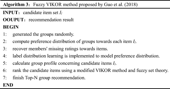
• Fuzzy VIKOR method proposed by Guo et al. (2018) (abbreviated as VIKOR). In this research, SVM method is conducted to model user preference, and then an improved VIKOR method is proposed to perform the group recommendation events. The pseudocode of the method is listed in Algorithm3.

  

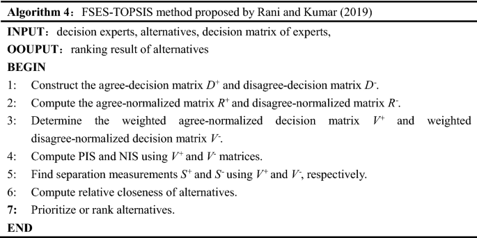
• FSES-TOPSIS approach proposed by Rani and Kumar (2019) (abbreviated as TOPSIS). In this research, TOPSIS along with Fuzzy Soft Expert Set (FSES) was applied to enable students to rank the faculty members based on their previous performance. The pseudocode of the method is listed in Algorithm4.

  

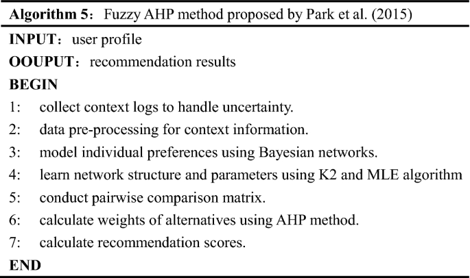
• Fuzzy AHP approach proposed by Park et al. (2015) (abbreviated as AHP). The Bayesian network is utilized to characterize the preferences of users, while the evaluation and recommendation of the alternatives are performed using AHP model. The pseudocode of the method is listed in Algorithm 5.

  

The similarity of the four methods is that the group preferences are generated based on individual preferences, and then the multi-attribute decision making method is applied to rank the alternatives to generate the final recommendations.

The difference is that: (1) In the Fuzzy VIKOR model, the SVM approach is employed to fit individual preferences, and objective weights are then applied to aggregate the indicators. However, the VIKOR method can only achieve better fits with large sample sizes; (2) The FSES-TOPSIS method assembles individual preferences into group preferences by fuzzy soft expert set and the indicators are integrated using objective weights. However, the TOPSIS approach requires decision makers to provide agree fuzzy value and disagree fuzzy value for the alternatives, which limits the input data for the model; (3) The fuzzy AHP model is used to integrate individual preferences. Although both subjective and objective weights of uses is considered in the AHP method, it is complicated to implement due to multiple interactions with decision users and the process is tedious.

Compared with the three models, the proposed combined weighting based group recommendation model incorporates both subjective and objective weights of individuals to generate group preferences based on clustering algorithm, which offers the superiority in terms of simplicity, convenient calculation and ease of implementation irrespective of sample size.

Table 8 presents the weights obtained using various methods, from which it can be concluded that regardless of the methods employed, criteria $c_{4}$ always gain the highest weight, with the value greater than 0.3, which means that performance is the most important criteria in the “CAMP” evaluation system. The distinction between the four methods exists in the inconsistent weighting of the first three criteria. The proposed combined weighting based LSGDM method is relatively uniform in terms of weight assignment, and there is no extreme case of favoring one attribute over another, which is also an advantage of the combined weighting method.

Table 8 Criteria weighting of different methods

Table 9 presents the alternative ranking results and group satisfaction obtained using different group recommendation methods. In terms of alternative ranking, among the recommendation results of the four models, the alternative ranking results of the model proposed in this paper are consistent with the VIKOR model and much closer to the TOPSIS model, while there are significant differences with the results of the AHP method. The main reason is that there are many subjective operations in the process of implementing the AHP model, which leads to major deviations in the results.

Table 9 Alternative ranking results and group satisfaction of different methods

In terms of group satisfaction, it seems that the proposed LSGDM-based group recommendation model in this study yields the highest group satisfaction of 0.4326, while the group satisfaction of the AHP, TOPSIS model is 0.4208, and VIKOR models was 0.391, 0.4208, and 0.4271, respectively. This indicates that the proposed LSGDM-based group recommendation model exhibits a better performance.

5 Conclusion

The rise of MOOC has promoted the open sharing of learning resources and facilitated people’s learning but has also led to a serious information overload problem. People fail to select a suitable course from the massive courses to satisfy the demands of individuals or groups. Therefore, a combined weighting based LSGDM method for MOOC group recommendations is proposed in this study. First, in accordance with the MOOC operation mode, we decompose the course content into three stages, namely pre-class, in-class, and post-class, and then the "CAMP" evaluation framework is constructed. Second, the PL-CRITIC method is employed to obtain the objective weighting of the criterion. Meanwhile, the word embedding model is utilized to vectorize online reviews, and the subjective weighting of the criteria are acquired by calculating the text similarity. Then the combined weighting of this study can be obtained by fusing the subjective and objective weighting. Further, the PL-MULTIMIIRA approach and Borda rule is employed to rank the alternatives for group recommendation. Based on this, an easy-to-use formula for group satisfaction was proposed to evaluate the effect of the group recommendation model. Finally, we conduct a case study by applying the LSGDM-based model to group recommendations for statistical MOOCs. Sensitivity and comparative analyses were carried out to verify the robustness and effectiveness of the proposed method.

The method proposed in this study is effectively applied to MOOC group recommendations, but shortcomings still exist. The calculation of online review-based weights requires construction of a text corpus. However, subjectivity exists in the construction of the text corpus, which may lead to a bias in the results. In future research, we will explore filling missing values in the recommendation model based on the distribution of the data.

Appendices

Appendix 1

Students are the main users of statistical MOOC, therefore, we choose a group of 20 students to make recommendations. The process is as follows: more than 1000 college students from different universities participated in a student science and technology competition held in 2021. A total of 136 students signed up for the group recommendation experiment on a voluntary basis. Among 136 students, 20 students were finally selected according to the distribution of colleges and universities, the participation of statistical MOOC and other factors. The personal information of 20 students is shown in Table

Table 10 The personal information of 20 students

10.

In addition, the main work of this paper is to recommend statistical MOOC based on user comments. Consider the same person may perform multiple reviews (including that the same person may make multiple comments using different IDs), or too few comments may affect the robustness of recommendation result. Hence, after analyzing the relationship between the number of comments and the cumulative number of course participants, we chose 8 statistics MOOCs with the cumulative number of course participants exceeding 1000 as the candidate course.

Appendix 2

References

Aher SB, Lobo LMRJ (2013) Combination of machine learning algorithms for recommendation of courses in e-learning system based on historical data. Knowl-Based Syst 51(10):1–14
Alturkistani A, Lam C, Foley K, Stenfors T, Blum ER, Van Velthoven MH, Meinert E (2020) Massive open online course evaluation methods: systematic review. J Med Internet Res 22(4):e13851
Brauers WKM, Zavadskas EK (2010) Project management by MULTIMOORA as an instrument for transition economies. Technol Econ Dev Econ 16(1):5–24
Chen S, Zhang C, Zeng S, Wang Y, Su W (2022) A probabilistic linguistic and dual trust network-based user collaborative filtering model. Artif Intell Rev 56(1):1–27
Diakoulaki D, Mavrotas G, Papayannakis L (1995) Determining objective weights in multiple criteria problems: the critic method. Comput Oper Res 22(7):763–770
Doo MY, Zhu M, Bonk CJ, Tang Y (2019) The effects of openness, altruism and instructional self-efficacy on work engagement of MOOC instructors. Br J Edu Technol 51(3):743–760
EADTU (2008) E-xcellence+: European wide introduction of QA in e-learning; a benchmarking approach. https://www.eurashe.eu/library/quality-he/Ib.5%20-%20Ubachs.pdf
Esteban A, Zafra A, Romero C (2019) Helping university students to choose elective courses by using a hybrid multi-criteria recommendation system with genetic optimization. Knowl-Based Syst 194(4):370–385
Fidalgo-Blanco Á, Sein-Echaluce ML, García-Peñalvo FJ (2016) From massive access to cooperation: lessons learned and proven results of a hybrid xMOOC/cMOOC pedagogical approach to MOOCs. Int J Educ Technol High Educ 13(1):1–13
Ghauth KI, Abdullah NA (2010) Learning materials recommendation using good learners’ ratings and content-based filtering. Educ Tech Res Dev 58(6):711–727
Guo Z, Tang C, Tang H, Fu Y, Niu W (2018) A novel group recommendation mechanism from the perspective of preference distribution. IEEE Access 6:5865–5878
Hu X, Jiang T, Wang M (2022) A hybrid recommendation model for online learning. Int J Robot Autom 37(5):453–459
Jansen RS, Van Leeuwen A, Janssen J, Conijn R, Kester L (2020) Supporting learners ’ self-regulated learning in massive open online courses. Comput Educ 146(4):103771
Jing X, Tang J (2017) Guess you like: course recommendation in MOOCs. In: Proceedings of the international conference on web intelligence (WI '17). Association for Computing Machinery, 783–789
Jordan K (2015) Massive open online course completion rates revisited: assessment, length and attrition. Int Rev Res Open Distrib Learn 16(3):341–358
Krishnan AR, Kasim MM, Hamid R, Ghazali MF (2021) A modified CRITIC method to estimate the objective weights of decision criteria. Symmetry 13(6):973
Lauren P, Qu G, Yang J, Watta P, Huang G-B, Lendasse A (2018) Generating word embeddings from an extreme learning machine for sentiment analysis and sequence labeling tasks. Cognit Comput 10(4):625–638
Lee D, Watson SL, Watson WR (2019) Systematic literature review on self-regulated learning in massive open online courses. Australas J Educ Technol 35(1):28–41
Li S, Wang S, Du J, Pei Y, Shen X (2021) MOOC learners’ time-investment patterns and temporal-learning characteristics. J Comput Assist Learn 38(1):152–166
Li X, Li X, Tang J, Wang T, Zhang Y, Chen H (2020) Improving deep item-based collaborative filtering with Bayesian personalized ranking for MOOC course recommendation. In: International conference on knowledge science, engineering and management, 247–258
Lin HF (2010) An application of fuzzy AHP for evaluating course website quality. Comput Educ 54(4):877–888
Lu OH, Huang JC, Huang AY, Yang SJ (2017) Applying learning analytics for improving students engagement and learning outcomes in an MOOCs enabled collaborative programming course. Interact Learn Environ 25(2):220–234
Luo D, Zeng S, Chen J (2020) A probabilistic linguistic multiple attribute decision making based on a new correlation coefficient method and its application in hospital assessment. Mathematics 8(3):340
Macleod H, Sinclair C, Haywood J, Woodgate A (2016) Massive open online courses: designing for the unknown learner. Teach High Educ 21(1):13–24
Margaryan A, Bianco M, Littlejohn A (2015) Instructional quality of massive open online courses (MOOCs). Comput Educ 80:77–83
Milligan C, Littlejohn A (2014) Supporting professional learning in a massive open online course. Int Rev Res Open Distan Learn 15(5):197–213
MOE of China (2022) China ranks first in world in numbers of MOOCs and viewers. http://en.brnn.com/n3/2022/0601/c415019-10104235.html
Murad DF, Heryadi Y, Isa SM, Budiharto W (2020) Personalization of study material based on predicted final grades using multi-criteria user-collaborative filtering recommender system. Educ Inf Technol 25(6):5655–5668
Nie Y, Luo H, Sun D (2020) Design and validation of a diagnostic MOOC evaluation method combining AHP and text mining algorithms. Interact Learn Environ 29(2):315–328
Okubo F, Yamashita T, Shimada A, Ogata H (2017) A neural network approach for students’ performance prediction. In: Proceedings of the seventh international learning analytics & knowledge conference, 598–599
Pang Q, Wang H, Xu Z (2016) Probabilistic linguistic term sets in multi-attribute group decision making. Inf Sci 369:128–143
Park H-S, Park M-H, Cho S-B (2015) Mobile information recommendation using multi-criteria decision making with Bayesian network. Int J Inf Technol Decis Mak 14(02):317–338
Pawlowski JM (2007) The quality adaptation model: adaptation and adoption of the quality standard ISO/IEC 19796–1 for the learning, education, and training. Educ Technol Soc 10:3–16
Pennington J, Socher R, Manning C (2014) GloVe: global vectors for word representation. In: Proceedings of the 2014 conference on empirical methods in natural language processing (EMNLP), 1532–1543
Rani BS, Kumar SA (2019) Recommendation system for under graduate students using FSES-TOPSIS. Int J Electr Eng Educ, 1–14. https://doi.org/10.1177/0020720919879385
Rezaeinia SM, Rahmani R, Ghodsi A, Veisi H (2018) Sentiment analysis based on improved pre-trained word embeddings. Expert Syst Appl 117:139–147
Sakketou F, Ampazis N (2020) A constrained optimization algorithm for learning GloVe embeddings with semantic lexicons. Knowl-Based Syst 195:105628
Shah D (2021) A decade of MOOCs: a review of MOOC stats and trends in 2021. https://www.classcentral.com/report/moocs-stats-and-trends-2021/
Sung YT, Chang KE, Yu WC (2011) Evaluating the reliability and impact of a quality assurance system for e-learning courseware. Comput Educ 57(2):1615–1627
Times (2012) College is dead. Long Live College! https://nation.time.com/2012/10/18/college-is-dead-long-live-college/
Tseng TH, Lin S, Wang YS, Liu HX (2022) Investigating teachers’ adoption of MOOCs: the perspective of UTAUT2. Interact Learn Environ 30(4):635–650
Tzeng GH, Chiang CH, Li CW (2007) Evaluating intertwined effects in e-learning programs: a novel hybrid MCDM model based on factor analysis and DEMATEL. Expert Syst Appl 32(4):1028–1044
Wang S, Wei G, Wu J, Wei C, Guo Y (2021) Model for selection of hospital constructions with probabilistic linguistic GRP method. J Intell Fuzzy Syst 40(1):1224–1259
Wu B (2021) Influence of MOOC learners discussion forum social interactions on online reviews of MOOC. Educ Inf Technol 26(3):3483–3496
Wu X, Liao H, Xu Z, Hafezalkotob A, Herrera F (2018) Probabilistic linguistic MULTIMOORA: a multicriteria decision making method based on the probabilistic linguistic expectation function and the improved borda rule. IEEE Trans Fuzzy Syst 26(6):3688–3702
Xu W, Zhou Y (2020) Course video recommendation with multimodal information in online learning platforms: A deep learning framework. Br J Edu Technol 51(5):1734–1747
Yousef AMF, Chatti MASchroeder U, Wosnitza M (2014) What drives a successful MOOC? An empirical examination of criteria to assure design quality of MOOCs. In: 2014 IEEE 14th international conference on advanced learning technologies, 44–48
Zeng S, Baležentis A, Su WH (2013) The multi-criteria hesitant fuzzy group decision making with MULTIMOORA method. Econom Comput Econom Cybernet Stud Res 47(3):171–184
Zeng S, Zhang N, Zhang C, Su W, Carlos LA (2022) Social network multiple-criteria decision-making approach for evaluating unmanned ground delivery vehicles under the pythagorean fuzzy environment. Technol Forecast Soc Chang 175:121414
Zhang C, Chen C, Streimikiene D, Balezentis T (2019) Intuitionistic fuzzy MULTIMOORA approach for multi-criteria assessment of the energy storage technologies. Appl Soft Comput 79:410–423
Zhang C, Wang Q, Zeng S, Baležentis T, Štreimikienė D, Ališauskaitė-Šeškienė I, Chen X (2018) Probabilistic multi-criteria assessment of renewable micro-generation technologies in households. J Clean Prod 212:582–592
Zhang M, Zhang C, Shi Q, Zeng S, Balezentis T (2022) Operationalizing the telemedicine platforms through the social network knowledge: an mcdm model based on the cipfohw operator. Technol Forecast Soc Chang 174:121303
Zhang H, Yang H, Huang T, Zhan G (2017) DBNCF: personalized courses recommendation system based on DBN in MOOC environment. Int Symp Educ Technol (ISET) 2017:106–108
Zhu Q, Wang S, Cheng B, Sun Q, Yang F, Chang RN (2018) Context-aware group recommendation for point-of-interests. IEEE Access 6:12129–12144
Acknowledgements
This work was supported by the project of the National Social Science Fund of China (22ATJ003, 21ATJ010, 20 CTJ016).
Author information
Authors and Affiliations
Corresponding author
Additional information
Publisher's Note
Springer Nature remains neutral with regard to jurisdictional claims in published maps and institutional affiliations.