Organising LTL monitors over distributed systems with a global clock

Abstract

Users wanting to monitor distributed systems often prefer to abstract away the architecture of the system by directly specifying correctness properties on the global system behaviour. To support this abstraction, a compilation of the properties would not only involve the typical choice of monitoring algorithm, but also the organisation of submonitors across the component network. Existing approaches, considered in the context of LTL properties over distributed systems with a global clock, include the so-called orchestration and migration approaches. In the orchestration approach, a central monitor receives the events from all subsystems. In the migration approach, LTL formulae transfer themselves across subsystems to gather local information. We propose a third way of organising submonitors: choreography, where monitors are organised as a tree across the distributed system, and each child feeds intermediate results to its parent. We formalise choreography-based decentralised monitoring by showing how to synthesise a network from an LTL formula, and give a decentralised monitoring algorithm working on top of an LTL network. We prove the algorithm correct and implement it in a benchmark tool. We also report on an empirical investigation comparing these three approaches on several concerns of decentralised monitoring: the delay in reaching a verdict due to communication latency, the number and size of the messages exchanged, and the number of execution steps required to reach the verdict.

Appendices

Appendix 1: Proofs

In this appendix, we provide the proofs for the propositions, lemmata, and the theorem of this paper.

Proposition 1

(Maximum level of nested distributions) $\forall \varphi \in \text{ LTL } \cdot {{\mathrm{dpth}}}_D({{\mathrm{net}}}(\varphi ))\le {{\mathrm{dpth}}}(\varphi )$.

Proof

The proof follows by induction on the structure of $\varphi$:

$\square$

Proposition 2

$\forall \varphi \in \text{ LTL } \cdot {{\mathrm{msg}}}^{\circ }({{\mathrm{net}}}(\varphi )) = \varphi$.

Proof

The proof follows by induction on the structure of the LTL formula.

¹⁷ $\square$

Lemma 1

(Correctness for one step under fully instantaneous communication)

$$\begin{aligned} \forall \varphi \in \text{ LTL }, \forall \sigma \in \varSigma \cdot \text {prog}(\varphi ,\sigma ) \simeq {{\mathrm{msg}}}^{\circ }({{\mathrm{alg}}}({{\mathrm{net}}}(\varphi ), \sigma )) \end{aligned}$$

The verdict reached by choreographed monitoring under fully instantaneous communication is the same as the one reached under standard progression with global view of events.

Proof

Since we assume fully instantaneous communication, in this proof we will ignore the algorithm’s communication mechanism and focus on part 5 of the algorithm, i.e., the respawning and distributed progression mechanism.

The proof follows by induction on the distribution structure, i.e., the linkages within the network memory, of $M = {{\mathrm{alg}}}({{\mathrm{net}}}(\varphi ),\sigma )$ with corresponding initial network N:

• Base case: Network of M has no linkages

  We note that when M has no distribution, ${{\mathrm{compute\_respawn}}}(N) = \emptyset$. Furthermore, ${{\mathrm{{{{\mathrm{prog}}}_{ t}}}}}$ behaves exactly as $\text {prog}$ in the non-distribution cases. Therefore, the base case follows by the inductive hypothesis and these observations.

• Inductive case: Formula of M has distribution linkages

  Due to the inductive hypothesis, which establishes a correspondence between the existing distribution placeholders in the formulae and the existing formulae being monitored in the network, we only need to prove that these maintain their correspondence and that new ones also correspond.

  • Case: Existing linkages of the form correspond to $M^t_{i,j}$

    We note that the t in and $M^t_{i,j}$ match and are not altered until the messaging system transmits the contents of $M^t_{i,j}$, meaning that the correspondence is maintained.

  • Case: New linkages of the form correspond to new formulae $M^t_{i,j}$ By case-by-case analysis of ${{\mathrm{{{{\mathrm{prog}}}_{ t}}}}}$, we note that there are only two means of introducing new in the formula: either within the $\mathbf{X}$ operator or within the $\mathbf{U}$ operator. Correspondingly, we note that by analysis of ${{\mathrm{compute\_respawn}}}$, there are only two means of introducing new $M^t_{i,j}$ in the formula: either within the $\mathbf{X}$ operator or within the $\mathbf{U}$ operator.

  • Case: Deleted linkages of the form , correspond to discarded formulae $M^t_{i,j}$ Following progression and simplification, a number of distribution propositions may be discarded. Part 7 of the algorithm is responsible for sending corresponding kill messages which are correspondingly handled by part 3. Conversely, if a cell $M^t_{i,j}$ reaches a verdict, part 8 of the algorithm is responsible for sending a verdict message to the corresponding distribution propositions and discarding the cell. Such a message is in turn handled by part 2 of the algorithm which replaces the placeholder with the verdict. Once more this preserves the correspondence of placeholders and cells.

$\square$

Lemma 2

(Correctness under fully instantaneous communication) Lifting Lemma 1 to trace of events, a trace of events still yields correct result when using the choreographed monitoring approach:

$$\begin{aligned} \forall \varphi \in \text{ LTL }, \quad \forall u \in \varSigma ^{*} \cdot \text {prog}(\varphi ,u) \simeq {{\mathrm{msg}}}^{\circ }({{\mathrm{alg}}}({{\mathrm{net}}}(\varphi ), u)) \end{aligned}$$

Proof

The proof follows by induction on the trace structure.

• Base case: An empty trace—$\text {prog}(\varphi ,\varepsilon ) \simeq {{\mathrm{msg}}}^{\circ }({{\mathrm{alg}}}({{\mathrm{net}}}(\varphi ), \varepsilon )$

  

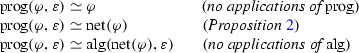
• Inductive case: An additional trace element—$\text {prog}(\varphi ,{{\mathrm{u}}}{{\mathrm{\cdot }}}\sigma ) \simeq {{\mathrm{msg}}}^{\circ }({{\mathrm{alg}}}({{\mathrm{net}}}(\varphi ), {{\mathrm{u}}}{{\mathrm{\cdot }}}\sigma )$ By the definitions of $\text {prog}$ and ${{\mathrm{alg}}}$, the statement can be reformulated to:

  $$\begin{aligned} \text {prog}(\text {prog}(\varphi ,{{\mathrm{u}}}),\sigma ) \simeq {{\mathrm{msg}}}^{\circ }({{\mathrm{alg}}}({{\mathrm{alg}}}({{\mathrm{net}}}(\varphi ), {{\mathrm{u}}}), \sigma ) \end{aligned}$$

  This follows by Lemma 1.

$\square$

Proposition 3

(More defined) $\forall \varphi \in \text{ LTL }_D,\forall \varphi '\in \text{ LTL } \cdot \varphi \succeq \varphi ' \implies \varphi =\varphi '$.

Proof

$\square$

Lemma 3

For all possible network memories, full messaging yields more defined formulae than verdict-only, time-stepped messaging: $\forall M \in {\mathscr {M}}\cdot {{\mathrm{msg}}}^{\circ }(M) \succeq {{\mathrm{{{\mathrm{msg}}}^{v}}}}(M)$.

Proof

By choosing the values of corresponding ${{\mathrm{msg}}}^{\circ }(M_{i,j})$ for undefined assignments of ${{\mathrm{{{\mathrm{msg}}}^{v}}}}(M)$, we would have $A({{\mathrm{{{\mathrm{msg}}}^{v}}}}(M))= {{\mathrm{msg}}}^{\circ }(M)$, which by definition of $\succeq$ lead us to conclude ${{\mathrm{msg}}}^{\circ }(M) \succeq {{\mathrm{{{\mathrm{msg}}}^{v}}}}(M)$ as required. $\square$

Theorem 1

(Correctness of verdict-only time-stepped messaging) If a verdict is reached when using verdict-only messaging, then the verdict is correct: $\forall \varphi \in \text{ LTL }, {{\mathrm{u}}}\in \varSigma ^{*} \cdot {{\mathrm{{{\mathrm{msg}}}^{v}}}}({{\mathrm{alg}}}({{\mathrm{net}}}(\varphi ),{{\mathrm{u}}})) \in \{\top ,\bot \}\implies {{\mathrm{{{\mathrm{msg}}}^{v}}}}({{\mathrm{alg}}}({{\mathrm{net}}}(\varphi ),{{\mathrm{u}}}))\simeq \text {prog}(\varphi ,{{\mathrm{u}}})$

Proof

The proof follows directly from Lemma 1, Proposition 3, and Lemma 3. $\square$

Corollary 1

(Correspondence of verdicts) If the decentralised semantics assigns a verdict to a trace-formula pair, then the $\text{ LTL } _3$ semantics assigns the same verdict: if ${{\mathrm{verdict}}}_{{ chor }}(u, \varphi ) \in \{\top ,\bot \}$ then ${{\mathrm{verdict}}}_{{ chor }}(u, \varphi ) = u \models _3 \varphi$.

Proof

The proof follows directly from Theorem 1. $\square$

Appendix 2: Plots for the visualisation of the results of the experiments

Recall that the experiments described in Sect. 7 aim at benchmarking and comparing the performance of the three decentralised monitoring algorithms (orchestration, migration, and choreography) along four metrics: the delay induced by decentralised monitoring, the number and size of messages exchanged by monitors, and number of progressions that monitors need to carry out to find a verdict (see Sect. 7 for the description of the metrics and objectives of the experiments).

In this section, we provide plots for the complementary visualisation of the results of the first and second experiments described in Sect. 7. For each metric, in each plot, we display information on the value of the metric according to formula size for the first experiment and according to specification pattern for the second experiment. For each metric, we provide three plots: (what is referred to as) a custom plot, a box plot, and a scatter plot.

1.1 Description of the plots

Custom plots report the average value (circle) and median (cross mark) of the metric. Moreover, the 99% confidence intervals of the means are depicted as crossbars centred around the mean value of the metric. In addition, to facilitate the visualisation and comparison of the algorithms based on the obtained average values, the symmetry or asymmetry of the metric value distribution can be hinted by inspecting the difference between the average and median values.

Box plots intuitively focus on “the main cases” and their dispersion. They also confirm the a(symmetry) of the distributions of observations hinted with custom plots. More precisely, recall that in a box plot the upper and lower “hinges” mark the first and third quartiles respectively. The line inside the box marks the second quartile (i.e., the median). Moreover, box plots are Tukey ones where the upper whisker extends up to the last values inside the upper inner fence, i.e., the highest value that lies within 1.5 times the inter-quartile range to the third quartile; and the lower whisker extends down to the last value inside the lower inner fence, i.e., the lowest value within 1.5 times the inter-quartile range to the first quartile. Outliers (i.e., values lower than the lower whisker and greater than the upper whisker) are not displayed.

Scatter plots display the values obtained for the metrics for all samples. They provide a global view of the obtained values and can be useful to estimate the number of outliers and their “distance to the middle values”. Horizontal jittering is applied to facilitate the estimation of the density of points.

Figures 6, 7, 8, and 9 contain the plots for the visualisation of the results of Experiment 1, for unbiased and biased formula generation. Figures 10, 11, 12, and 13 contain the plots for the visualisation of the results of Experiment 2.

Fig. 6

Visualisation of the results (reported in Table 2) obtained for the trace length ($|\mathrm{tr}|$ in ordinate) with the experiment varying the size of formulae ($|\varphi |$ in abscissa). a Custom plot—unbiased formula generation. b Custom plot—biased formula generation. c Boxplot—unbiased formula generation, d Box plot—biased formula generation. e Scatter plot— unbiased formula generation. f Scatter plot—biased formula generation

Fig. 7

Visualisation of the results (reported in Table 2) obtained for the number of messages ($\#\mathrm{msg}$ in ordinate) with the experiment varying the size of formulae ($|\varphi |$ in abscissa). a Custom plot— unbiased formula generation. b Custom plot—biased formula generation. c Box plot—unbiased formula generation. d Box plot—biased formula generation. e Scatter plot— unbiased formula generation. f Scatter plot—biased formula generation

Fig. 8

Visualisation of the results (reported in Table 2) obtained for the size of messages ($|\mathrm{msg}|$ in ordinate) with the experiment varying the size of formulae ($|\varphi |$ in abscissa). a Custom plot— unbiased formula generation. b Custom plot—biased formula generation. c Box plot—unbiased formula generation. d Box plot—biased formula generation. e Scatter plot— unbiased formula generation. f Scatter plot—biased formula generation

Fig. 9

Visualisation of the results (reported in Table 2) obtained for the number of progressions ($\#\mathrm{prog}$ in ordinate with the experiment varying the size of formulae ($|\varphi |$ in abscissa). A base-10 logarithmic scale is used for the ordinate axis of scatter plots. a Custom plot—unbiased formula generation. b Custom plot - biased formula generation. c Box plot—unbiased formula generation. d Box plot—biased formula generation. e Scatter plot—unbiased formula generation. f Scatter plot—biased formula generation

Fig. 10

Visualisation of the results (reported in Table 3) obtained for the trace length ($|\mathrm{tr}|$ in ordinate) with the experiment varying the pattern of formulae (in abscissa). a Custom plot. b Box plot. c Scatter plot

Fig. 11

Visualisation of the results (reported in Table 3) obtained for the number of messages ($\#\mathrm{msg}$ in ordinate) with the experiment varying the pattern of formulae (in abscissa). a Custom plot. b Box plot. c Scatter plot

Fig. 12

Visualisation of the results (reported in Table 3) obtained for the size of messages ($|\mathrm{msg}|$ in ordinate) with the experiment varying the pattern of formulae (in abscissa). a Custom plot. b Box plot. c Scatter plot

Fig. 13

Visualisation of the results (reported in Table 3) obtained for the number of progressions ($\#\mathrm{prog}$ in ordinate) with the experiment varying the pattern of formulae (in abscissa). a Custom plot. b Box plot. c Scatter plot (with base-10 logarithmic scale for the ordinate axis)

1.2 Using the plots to analyse data

We now describe how to use the plots to draw conclusions from the experimental data. We refrain from examining each metric for each formula size and specification pattern but rather recall general methods to analyse the plots and mention some of the interesting cases. The plots confirm and refine the trends mentioned in Sects. 7.4, 7.5, and 7.6.

The relative positions of the mean and median give hints on data skewness. A positive (resp. negative) value for the difference between the mean and median can hint a positive (resp. negative) skew.

Moreover, box plots indicate centrality (with the median), spread (the size of the box), symmetry or skewness of data, and tail length and shape of the distribution (with the relative lengths of the whiskers and box). Positive (resp. negative) skewness is characterised by a median in the lower (resp. upper) part of the box and an upper (resp. lower) whisker that is longer than the lower (resp. upper) whisker. However, we note that the above rule does not cover all the cases and other situations may arise, for instance for the number of messages obtained with the choreography algorithm for random formulae of size 5 where the mean and median are close to each other, the median is in the upper part of the box, and the lower whisker is inexistant. Hence, both the median position and the lengths of whiskers have to be examined to draw conclusions on the distribution of values. For instance:

• The number of messages obtained for response formulae (cf. Fig. 11b) has no skew for the three algorithms,

• The trace length and number of progressions obtained for (unbiased and biased) random formulae (cf. Fig. 6 and 9) has a positive skew,

• None of the obtained distributions for the metrics has a negative skew.

Scatter plots help visualising the positions and density of outliers compared to the “main values” for each distribution. For instance, for the trace lengths obtained when monitoring randomly-generated formulae, the number and positions of outliers seem to be the same for the three algorithms. For the number of messages obtained when monitoring formulae with unbiased random formula generation, choreography has more and further outliers than orchestration, while the situation is reversed when formulae are obtained with biased formula generation. For Experiment 2 (related to specification patterns), examining the scatter plots with far outliers, we can notice that, for some precedence chain formulae, choreography was defeated in terms of number of progressions while it performed similarly or better for trace length and size of messages. Finally, a question that arose was whether the outliers were for the same formulae across all algorithms. After observing the scatter plots and the data set obtained from the experiments, we confirm that this is generally the case, meaning that outliers reflect the differences between formulae rather than algorithms.

References

Baier C, Katoen J (2008) Principles of model checking. MIT Press, Cambridge
Barringer H, Rydeheard DE, Havelund K (2010) Rule systems for run-time monitoring: from Eagle to RuleR. J Log Comput 20(3):675–706
Bartocci E (2013) Sampling-based decentralized monitoring for networked embedded systems. In: 3rd international workshop on hybrid autonomous systems, EPTCS, vol 124, pp 85–99
Bauer A, Leucker M, Schallhart C (2010) Comparing LTL semantics for runtime verification. Log Comput 20(3):651–674
Bauer A, Leucker M, Schallhart C (2011) Runtime verification for LTL and TLTL. ACM Trans Softw Eng Methodol (TOSEM) 20(4):14
Bauer AK, Falcone Y (2012) Decentralised LTL monitoring. In: 18th international symposium on formal methods, LNCS, vol 7436. Springer, pp 85–100
Colombo C, Falcone Y (2014) Organising LTL monitors over distributed systems with a global clock. In: Proceedings of the 5th international conference runtime verification (RV 2014), Lecture notes in computer science. Springer, pp 140–155
Dwyer MB, Avrunin GS, Corbett JC (1999) Patterns in property specifications for finite-state verification. In: International conference on software engineering (ICSE). ACM, pp 411–420
Etessami K, Holzmann GJ (2000) Optimizing Büchi automata. In: Palamidessi C (ed) CONCUR 2000—concurrency theory, 11th international conference, University Park, PA, USA, August 22–25, 2000, Lecture notes in computer science, vol 1877. Springer, pp 153–167
Falcone Y, Cornebize T, Fernandez J-C (2014) Efficient and generalized decentralized monitoring of regular languages. In: Ábrahám E, Palamidessi C (eds) FORTE 2014: 34th IFIP international conference on formal techniques for distributed objects, components and systems, LNCS, vol 8461. Springer, pp 66–83
Falcone Y, Fernandez J, Mounier L (2012) What can you verify and enforce at runtime? Int J Softw Tools Technol Transf 14(3):349–382
Falcone Y, Havelund K, Reger G (2013) A tutorial on runtime verification. In: Broy M, Peled D, Kalus G (eds) Engineering dependable software systems, NATO science for peace and security series, D: Information and communication security, vol 34. IOS Press, pp 141–175
Francalanza A, Gauci A, Pace GJ (2013) Distributed system contract monitoring. J Log Algebr Program 82(5–7):186–215
Graf S, Peled D, Quinton S (2011) Monitoring distributed systems using knowledge. In: Bruni R, Dingel J (eds) Proceedings of the joint 13th IFIP WG 6.1 international conference and 31st IFIP WG 6.1, LNCS, vol 6722. Springer, pp 183–197
Gunzert M, Nägele A (1999) Component-based development and verification of safety critical software for a brake-by-wire system with synchronous software components. In: International symposium on SE for parallel and distributed systems (PDSE). IEEE, p 134
Harris D (2003) A taxonomy of parallel prefix networks. Signals Syst Comput 2:2213–2217
Havelund K, Goldberg A (2005) Verify your runs. In: Meyer B, Woodcock J (eds) Verified software: theories, tools, experiments, first IFIP TC 2/WG 2.3 conference, VSTTE 2005, Zurich, Switzerland, October 10–13, 2005, revised selected papers and discussions, Lecture notes in computer science, vol 4171. Springer, pp 374–383
Havelund K, Rosu G (2001) Monitoring programs using rewriting. In: 16th IEEE international conference on automated software engineering (ASE 2001), pp 135–143
Larrieu R, Shankar N (2014) A framework for high-assurance quasi-synchronous systems. In: Twelfth ACM/IEEE international conference on formal methods and models for codesign, MEMOCODE 2014, Lausanne, Switzerland, October 19–21, 2014. IEEE, pp 72–83
Leucker M, Schallhart C (2009) A brief account of runtime verification. J Log Algebr Program 78(5):293–303
Lynch WC (1968) Computer systems: reliable full-duplex file transmission over half-duplex telephone line. Commun ACM 11(6):407–410
Manna Z, Pnueli A (1992) The temporal logic of reactive and concurrent systems. Springer-Verlag New York Inc, New York
Mayr R, Clemente L (2013) Advanced automata minimization. In: Giacobazzi R, Cousot R (eds) The 40th annual ACM SIGPLAN-SIGACT symposium on principles of programming languages, POPL ’13, Rome, Italy, January 23–25, 2013. ACM, pp 63–74
Miller SP, Whalen MW, Cofer DD (2010) Software model checking takes off. Commun ACM 53:58–64
Pnueli A (1977) The temporal logic of programs. In: SFCS’77: Proceedings of the 18th annual symposium on foundations of computer science. IEEE Computer Society, pp 46–57
Pnueli A, Zaks A (2006) PSL model checking and run-time verification via testers. In: Misra J, Nipkow T, Sekerinski E (eds) FM 2006: formal methods, 14th international symposium on formal methods, Hamilton, Canada, August 21–27, 2006, Lecture notes in computer science, vol 4085. Springer, pp 573–586
Pnueli A, Zaks A (2008) On the merits of temporal testers. In: Grumberg O, Veith H (eds) 25 Years of model checking—history, achievements, perspectives, Lecture notes in computer science, vol 5000. Springer, pp 172–195
Pop T, Pop P, Eles P, Peng Z, Andrei A (2008) Timing analysis of the FlexRay communication protocol. Real-Time Syst 39:205–235
Rosu G, Havelund K (2005) Rewriting-based techniques for runtime verification. Autom Softw Eng 12(2):151–197
Sen K, Rosu G, Agha G (2003) Generating optimal linear temporal logic monitors by coinduction. In: Saraswat VA (ed) Advances in computing science—ASIAN 2003 programming languages and distributed computation, 8th Asian computing science conference, Mumbai, India, December 10–14, 2003, Lecture notes in computer science, vol 2896. Springer, pp 260–275
Sen K, Vardhan A, Agha G, Rosu G (2006) Decentralized runtime analysis of multithreaded applications. In: 20th parallel and distributed processing symposium (IPDPS). IEEE
Sokolsky O, Havelund K, Lee I (2012) Introduction to the special section on runtime verification. Int J Softw Tools Technol Transf 14(3):243–247
Somenzi F, Bloem R (2000) Efficient büchi automata from LTL formulae. In: Emerson EA, Sistla AP (eds) Computer aided verification, 12th international conference, CAV 2000, Chicago, IL, USA, July 15–19, 2000, Lecture notes in computer science, vol 1855. Springer, pp 248–263
Acknowledgments
The work reported in this article has been done in the context of the COST Action ARVI IC1402, supported by COST (European Cooperation in Science and Technology). The authors would like to thank Adrian Francalenza (U of Malta), Susanne Graf (Vérimag), and César Sanchez (IMDEA Madrid) for discussions the issue on simplifying \(\text{ LTL } \) formulae. The authors are grateful to the DataMill team at the University of Waterloo for providing us with such a nice experimentation platform. The authors gratefully thank the anonymous reviewers for their comments and suggestions allowing to improve the quality of this paper.
Author information
Authors and Affiliations
Corresponding author