Modelling Deposit Insurance Scheme Losses in a Basel 2 Framework

Abstract

This paper extends the existing literature on deposit insurance by proposing a new approach for the estimation of the loss distribution of a Deposit Insurance Scheme (DIS) that is based on the Basel 2 regulatory framework. In particular, we generate the distribution of banks’ losses following the Basel 2 theoretical approach and focus on the part of this distribution that is not covered by capital (tail risk). We also refine our approach by considering two major sources of systemic risks: the correlation between banks’ assets and interbank lending contagion. The application of our model to 2007 data for a sample of Italian banks shows that the target size of the Italian deposit insurance system covers up to 98.96% of its potential losses. Furthermore, it emerges that the introduction of bank contagion via the interbank lending market could lead to the collapse of the entire Italian banking system. Our analysis points out that the existing Italian deposit insurance system can be assessed as adequate only in normal times and not in bad market conditions with substantial contagion between banks. Overall, we argue that policy makers should explicitly consider the following when estimating DIS loss distributions: first, the regulatory framework within which banks operate such as (Basel 2) capital requirements; and, second, potential sources of systemic risk such as the correlation between banks’ assets and the risk of interbank contagion.

1 Introduction

Deposit insurance schemes (DIS) are set up with the purpose of providing depositors with the guarantee that their deposits will be (at least in part) repaid whenever a bank defaults. This guarantee, mainly aimed at preventing bank runs, is a contribution to the stability of the financial system. To perform this role, a DIS needs to have an adequate amount of funds at its disposal. Therefore, the estimation of the losses that can affect the deposits of the insured banks in different market scenarios is a key issue for a DIS and for regulators alike. The loss distribution of the DIS is, in conclusion, the key piece of information which is needed to assess the adequacy of its funds,¹ establish a funding target and derive the risk-based contributions that banks should pay to the DIS.

Despite the relevance of DIS loss distribution for policy decisions, it is striking that, given the extensive literature on deposit insurance, only a few studies have tried to estimate it (see Kuritzkes et al. 2005; Sironi et al. 2004). These studies have generally tried to do so by relying on structural credit risk models and market data to derive banks’ default probabilities, and then estimating the losses for the DIS in case of bank failures. This paper extends these analyses by proposing a new approach to estimating the DIS loss distribution. To our knowledge the approach we propose is the first that explicitly considers the link that exists between deposit insurance and the regulatory framework for capital requirements introduced by Basel 2. This is done in two ways.

First, our approach models the probability of default of a bank as the probability that its obligor’s losses exceed actual capital, which is given by its Basel 2 regulatory capital plus its excess capital, if any. As is well known, in the Basel 2 framework each bank has to satisfy a capital requirement that provides a buffer against unexpected losses at a specific level of statistical confidence, set by regulators at 99.9% (Basel Committee on Banking Supervision 2004, 2005). Therefore, in the Basel 2 regulatory framework the probability that banks default can be seen as the probability that banks’ losses fall in the tail of their loss distribution. This “tail risk” is equal to 0.1% whenever banks set their amount of capital at a level equal to their regulatory minimum (Repullo and Suarez 2004) or lower, as banks normally hold capital well in excess of the regulatory minimum (see, for example, Jokipii and Milne 2008, 2010; Stolz and Wedow 2009).

Second, we estimate the DIS loss distribution by aggregating individual bank losses computed according to the Basel 2 FIRB (Foundation Internal Rating Based) formula. To estimate the default probability of the bank’s obligors, which is needed in the FIRB formula, we propose a novel approach that leverages on publicly available regulatory capital information.

Hence, our model creates an explicit link between the two main pillars of the financial safety net for banks: capital requirements on the one hand, and deposit insurance schemes on the other. The relationship between these two safety net tools has been extensively analysed by a broad theoretical literature (see Santos 2000, for a survey). For instance, the moral hazard effect created by the establishment of unfairly priced deposit insurance schemes has generally been identified as one of the main reasons for the introduction of capital requirements for banks. Furthermore, whenever there are information frictions, the need to jointly consider the design of deposit insurance and capital requirements has generally been recognised (Santos 2000). In this paper we propose to go one step further and require that capital requirements should be explicitly considered in the estimation of the DIS loss distribution.

Our model also extends the existing literature on deposit insurance by taking into account how two major sources of systemic risk in the banking system affect the size and shape of the DIS loss distribution. The first source of systemic risk depends on the existence of a correlation between banks’ assets. This correlation may exist as a consequence of banks’ common exposure to the same borrower or, more generally, to a particular common influence of the business cycle. An adverse economic shock may therefore result in simultaneous multiple defaults on bank loans. The second source of systemic risk depends on the linkages existing between banks through the interbank lending market (interbank contagion). Hence, our methodology is closely related to recent models used to quantify the potential for systemic risk in the financial industry (Elsinger et al. 2006).

Under simplified assumptions, we apply our approach to 2007 data for a sample of Italian banks in order to assess the adequacy of the Italian DIS funding target. Our results suggest that the target fund established in 2007 for the Italian DIS can cover up to 98.96% of its potential losses. Furthermore, while interbank contagion does not produce an overall shift in the Italian DIS loss distribution, it does cause a large increase in its right tail, potentially leading to the collapse of the entire Italian banking system. It follows that a favourable assessment of the adequacy of the existing Italian deposit insurance system must exclude exceptionally bad market conditions involving substantial contagion between banks via the interbank lending market. Moreover, the paper underlines the need for supervisory authorities to treat contagion risk as a key element when assessing the fund adequacy of a DIS and, more generally, when designing the overall financial safety net.

The rest of this paper is organized as follows. The second section presents a brief review of the literature, while the third describes our approach to modelling DIS loss distribution in a Basel 2 framework. The fourth section describes the sample and the variables used in the analysis, and provides some indications on the characteristics of the Italian DIS. The fifth section discusses the results of applying our methodology to a sample of Italian banks. The sixth section sets out conclusions.

2 Literature review

This paper is closely related to the literature that seeks to quantify the DIS loss distribution and to estimate the optimal size of the DIS funds, knowing banks’ probabilities of default. The literature has generally applied two alternative methodologies in order to assess whether DIS funds are adequate. The first methodology is based on option pricing theory, originally proposed by Merton (1974) to model risk-based premium in DIS, and later implemented by Markus and Shaked (1984) and Ronn and Verma (1986). This approach relies on structural credit risk models to derive the banks’ probability of default and, typically, on simulation-based methods to quantify the DIS loss distribution (Kuritzkes et al. 2005; Sironi et al. 2004). The second methodology, which is less common in the DIS literature, adopts instead a reduced-form model, drawn from the pricing of fixed-income securities under default risk, adjusted to be tractable for banks without market debts (Duffie et al. 2003).

One of the major differences between these two approaches is in the way they define the event of default. In the structural approach, default is identified as the event occurring when the market value of the bank’s assets falls below a certain threshold, generally determined by the value of the bank’s liabilities. Conversely, when the reduced form model is used, as pointed out by Duffie et al. (2003), default is defined as a stopping time the intensity of which depends on covariates such as leverage, credit rating or macroeconomic conditions.

An application of the first methodology to deposit insurance is provided by Kuritzkes et al. (2005), for the US context. They quantify the loss distribution faced by the FDIC, by applying the Merton model to estimate changes in banks’ credit quality. The loss distribution is derived through Monte Carlo simulations, where the changes in the PD are a function of a systematic risk factor (dependent on macro variables) and of a bank-specific idiosyncratic component. Their results suggest that the FDIC reserves are sufficient to cover 99.85% of the loss distribution related to the fund’s 8,571 member banks.

Sironi et al. (2004) apply a somewhat similar approach to the 15 largest Italian listed banks. Their estimated loss distribution makes it possible to quantify the loss rate for every possible confidence interval and a multiplier that, when applied to the unexpected loss, computes the loss corresponding to the desired confidence interval. Their study highlights that, while the most risky banks give a greater contribution in terms of expected loss, the larger banks make the greater contribution in terms of unexpected loss. As a result, the difference between an insurance premium based only on expected loss and one built on unexpected loss can be substantial for banks that represent the larger exposures.

Unlike Kuritzkes et al. (2005) and Sironi et al. (2004), Dev et al. (2006) propose a structural model for deposit insurance premia that is characterised by an analytical solution rather than obtained by means of a simulation-based approach. Their modelling framework explicitly takes into account the liability structure of banks, by distinguishing insured and uninsured deposits from senior secured debts, and introduces the correlation between PD and LGD as a determinant of deposit insurance premia.²

Duffie et al. (2003) present an application of reduced form models to DIS, inspired by the pricing of fixed-income securities subject to default risk. The fair-market insurance rate for a given bank is approximated as the bank’s short term credit spread times the ratio of the insurer expected loss at failure per dollar of insured deposits to the bond investor’s expected loss at failure per dollar of principal. Furthermore, to overcome the possibility that financial institutions do not present market debts in their capital structure, Duffie et al. (2003) propose an alternative methodology based on a logit model of the bank’s default probability.

A further different approach has been proposed by Jarrow et al. (2006) that focus instead on the computation of countercyclical risk premium by modelling the unconditional distribution of the loss events, the asset size of the failing banks and the loss rate for the DIS in the case of bank defaults. In such a framework, the number of failures is derived by simulation, based on the historical failure experience of the FDIC. Their analysis suggests that any countercyclical policy is not costless. By contrast, a countercyclical rebate system produces an increase in the aggregate premium of about $9 billion over a period of 10 years.

Summing up, the existing literature that seeks to estimate the DIS loss distribution is mainly based on structural models for credit risk, which generally require market data in order to empirically apply the proposed methodology. This literature shows no sign of considering any link between banks’ capital requirements and the shape and size of the DIS loss distribution. As is fully explained in the following section, our approach differs from the existing literature in two major respects.

First, we estimate the DIS loss distribution on the basis of a framework that explicitly links two main pillars of the financial safety net, namely banks’ capital requirements and deposit insurance. More specifically, and unlike previous studies, we model the bank’s default probability as a tail risk (Repullo and Suarez 2004) that reflects bank capital strength and asset quality. To this end, we postulate that default takes place for each bank when the amount of its asset losses exceeds the bank’s capital requirements plus (if applicable) the bank’s excess capital.

Hence, given that under the Basel 2 accord capital requirements provide a buffer against unexpected losses at a level of statistical confidence set by regulators at 99.9%, whenever banks fix the amount of capital at the regulatory minimum they share the same probability of default equal to 0.1% (Repullo and Suarez 2004). However, banks normally hold capital well in excess of this minimum regulatory amount (see for example Jokipii and Milne 2008, 2010; Stolz and Wedow 2009). As a result, they also show different (lower than 0.1%) probabilities of default. On the basis of these default probabilities for banks, we design the losses stemming from banks and affecting the DIS, by using the Basel 2 FIRB formula.

Second, we explicitly take into account the impact of systemic risk that, as in DeBandt and Hartmann (2000), we assume as being generated by two different sources. The first source of systemic risk depends on the fact that banks have correlated assets, and thus that an economic shock has consequences for the financial system and the broader economy, simultaneously impacting a number of banks. The second source of systemic risk depends instead on the linkages between banks produced by the interbank lending market that can produce a default domino effect across the banking system (interbank contagion).

The relative importance of these two sources of systemic risk is assessed by Elsinger et al. (2006) in an analysis aimed at evaluating the potential for systemic risk in the Austrian banking industry. Their conclusion is that correlated portfolio exposures of banks are the major source of systemic risk, while contagion via the interbank lending market seems to be a rare event. Contrary to our analysis, the authors do not investigate the implications of their model for deposit insurance schemes, but focus instead on the consequences for a lender of last resort of these two channels of systemic risk.

3 Methodology

We estimate the loss distribution of a DIS in a simplified banking system where banks are exposed only to credit risk and are fully compliant with the FIRB Basel 2 minimum capital requirements. The analysis follows the steps summarised by Fig. 1.

Fig. 1

Steps of the analysis

• Step 1: Define the default point

  We start by defining when a bank defaults in a Basel 2 framework. More specifically, the new capital accord uses the Vasicek (see Vasicek 1987, 1991, 2002; and Gordy 2003) model to compute, for each obligor of the bank, its Value at Risk (VaR), which is the loss amount that is not expected to be exceeded within a given confidence level α and within a defined time horizon.³

  As banks are generally expected to cover their Expected Losses (EL) on an ongoing basis, i.e. by provisions and write-offs, Basel 2 requires banks to hold capital only to cover Unexpected Losses (UL). Therefore, as shown in Fig. 2 (and in accordance with the Basel 2 framework), we assume that a bank j defaults when obligor portfolio losses (L) exceed the sum of the expected losses (EL) and the total actual capital (CAP) given by the sum of its capital requirements plus the bank’s excess capital (if any); namely, when the following condition is satisfied:

  Fig. 2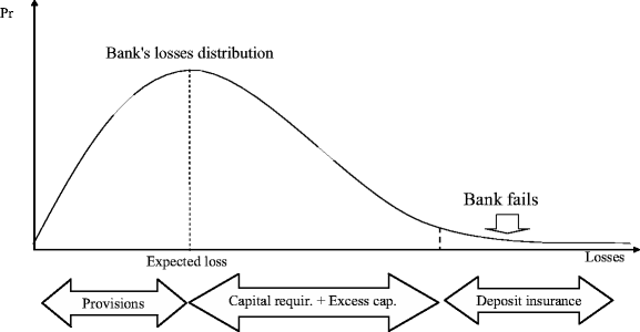

  

  Tail risk, Basel 2 and deposit insurance

  $$ {L_j} > E{L_j} + CA{P_j} $$

  (1)

  As detailed in the following section, we model the losses generated by the bank portfolio (L _j ) as a function of the creditworthiness of bank obligors. Thus, banks that hold the same amount of assets differ in their likelihood of failure when the risk of default of their obligors differs.⁴ However, this is not the only factor that determines differences in the risk of default across banks under the condition indicated by Eq. 1.

  More precisely, banks that show both an identical size and quality of the asset portfolio, may still show differences in default risk if they hold a different amount of capital (CAP _j ). In turn, this implies that bank default risk is a function of a bank’s capital strength.⁵

  Overall, the condition in Eq. 1 implies that the obligor credit quality and the bank capital strength are the two bank characteristics that have a direct influence on the bank default event.

• Step 2: Generate via Monte Carlo a sample of correlated bank’s asset losses

  According to Eq. 1, one of the key variables to identify when a bank defaults is the amount of asset losses. We quantify this amount via a Monte Carlo simulation. We simulate a sample of banks’ losses L _ij , for each bank j, and for each simulation i = 1,...,n, in the form of a (n × k) matrix, where n is the total number of simulations and k is the total number of banks in the system. The sample is generated using the same distribution for banks’ losses as used by Basel 2 in the FIRB approach. In particular, if we denote by α the probability of the loss being less than or equal to a certain amount x, we have:

  $$ \alpha = P\{ L \leqslant x\} = N\left[ {\frac{{\sqrt {{1 - R}} {N^{{_{{ - 1}}}}}(x) - {N^{{_{{ - 1}}}}}(PD)}}{{\sqrt {R} }}} \right] $$

  (2)

  where N is the normal cumulative density function, and R is the common pairwise correlation between obligors, specified as in Basel 2.

  With some algebra, we can express the loss x as a function of the probability α:

  $$ x = N\left[ {\frac{{\sqrt {R} {N^{{_{{ - 1}}}}}(\alpha ) + {N^{{_{{ - 1}}}}}(PD)}}{{\sqrt {{1 - R}} }}} \right] $$

  (3)

  In our model, denoting by L _ij the i _th realization of the maximum loss for bank j given a certain random value of probability α _ij , by PD _j the average probability of default of the asset portfolio of bank j, and by LGD the Loss Given Default, formula Eq. 3 reads:

  $$ {L_{{ij}}} = LGD \times N\left[ {\sqrt {{\frac{1}{{1 - R}}}} {N^{{_{{ - 1}}}}}(P{D_j}) + \sqrt {{\frac{R}{{1 - R}}}} {N^{{_{{ - 1}}}}}({\alpha_{{ij}}})} \right] $$

  (4)

  Assuming LGD ≠ 1, a sample of losses L _ij is generated via random shocks for N ⁻¹ (α), which is assumed to be normally distributed. The assumption of normal distribution is needed in order to reproduce the distribution of banks’ losses which is implied in Basel 2.

  To estimate the values of PDs needed in Eq. 4, we adopt a novel approach that is consistent with the Basel 2 regulatory framework. In particular, we compute a proxy of the quality of a bank obligor portfolio by inverting the Basel 2 FIRB capital requirement formula as described in Appendix. This can be done as the PD of a bank obligor is the only unknown variable: the capital requirement is known, and all other variables in the formula can be set to their regulatory values.

  The resulting estimate $PD_j^{ * }$, hereafter ImpliedObligorPD, represents a proxy of the average default probability of the obligor portfolio of bank j.

  Within this general framework, the model takes account of a first source of systemic risk, as banks have correlated exposures. This correlation exists either as a consequence of the banks’ common exposure to the same borrower or, more generally, to a particular common influence of the business cycle. We model the impact of this macroeconomic source of systemic risk by generating a correlated random shock on the basis of a correlation matrix among banks’ assets.

  Initially, for the sake of simplicity we assume that banks share the same value of asset correlation. Specifically, Sironi et al. (2004) found that the average asset correlation for a sample of Italian banks is around 50%. Hence, we use this value as initial input in our model. However, the assumption of a constant correlation across banks leaves out some firm heterogeneity and can influence the estimation of the DIS loss distribution.⁶ Therefore, we elaborate further on this point in the robustness section, where we consider alternative specifications of the correlation matrix.

• Step 3: Check which banks fail

  Once a sample of banks’ losses has been generated, these losses are used to determine which banks fail in each simulation. In particular, we check which banks fail according to the condition established by Eq. 1 and create, from a (n × k) matrix of losses, a matrix of failures which is a (n × k) matrix of zeros (no failure) and ones (failure).

• Step 4: Include interbank contagion risk.

  Next, we introduce into the model a second source of systemic risk, defined as the risk of contagion between banks though the interbank lending market. When a bank fails, its losses actually affect both the bank’s (insured) deposits and the interbank creditors,⁷ and we must consider that a bank may also fail because the losses produced through the interbank market have triggered a domino effect on other banks.

  We model the contagion across k banks (of which j failed) by assuming a proportional distribution of the interbank losses of a defaulted bank’s to the remaining interbank creditor banks. For instance, if bank j fails, we assume that the losses that bank j passes to the remaining bank h are proportional to the credit share of bank h in the interbank market. The loss incurred by bank h can then be written as follows:

  $$ IBlos{s_h}(j) = IB_j^{ - }\frac{{IB_h^{ + }}}{{\sum\limits_{{k \ne j}} {IB_k^{ + }} }} $$

  (5)

  where $IB_j^{ - }$ is the debt exposure of bank j in the interbank market and $IB_h^{ + }$is the creditor exposure of bank h in the same market. The total loss of bank h due to the interbank contagion effect is obtained as:

  $$ IBlos{s_h} = \sum\limits_j {IB_j^{ - }\frac{{IB_h^{ + }}}{{\sum\limits_{{k \ne j}} {IB_k^{ + }} }}} $$

  (6)

  Then, the resulting loss of bank h will be given by the sum of the losses of its loan portfolio plus the losses suffered via the interbank market exposures.

  Once the matrix of bank losses has been completed, we check whether other banks fail due to the contagion effect. We repeat the procedure until no additional bank failure is produced, and build the final bank failure matrix. Notably, by modeling bank contagion, we introduce further elements of heterogeneity across banks as the banks’ default risk will now also depend on a bank net position in the interbank market.

• Step 5: Derive the DIS loss distribution

  The empirical DIS loss distribution is obtained as follows. For each simulated scenario we look at which banks fail and transfer to the DIS the total amount of its deposits. This, once again, corresponds to addressing a liquidity problem where we assume that the total loss of a defaulted bank is equal to its total liabilities (deposits).

  It is worth noting that the model can also be used to derive a proxy of the bank’s PD, namely BankPD (to be distinguished from its portfolio average PD, ImpliedObligorPD). This is derived as the ratio of the number of times a bank fails over the total number of simulated scenarios. Note that the BankPD results from the interaction between its asset quality (ImpliedObligorPD) and its capital strength.

4 Sample, variables of the analysis and main characteristics of the Italian DIS

The model described in the previous section has been applied to unconsolidated accounting data for a sample of 494 Italian banks for year 2007. Data are drawn from the ABIBANK dataset managed by the Italian Banking Association (ABI). The variables employed in the analysis are summarized in Table 1, where we show some basic descriptive statistics. ABIBANK dataset ensures a proper coverage of the entire Italian banking system. According to the statistics provided by Bank of Italy, our sample accounts in fact for around 70% of the total DIS eligible deposits.⁸

Table 1 Summary statistics. This table reports descriptive statistics for our sample of 494 Italian banks for 2007. This sample represents around 70% in terms of total DIS eligible deposits. Amounts are in m€

The banks selected in our sample are covered by the safety net arrangement provided by the Italian deposit insurance system, which consists of two schemes. The first is the Fondo Interbancario di Tutela dei Depositi (FITD), established in 1987 as a voluntary consortium, and which is now a private mandatory consortium recognised by the Bank of Italy. The second is the Fondo di Garanzia per le Banche di Credito Cooperativo, established in 1997 for co-operative banks operating in Italy.

Both schemes are based on an ex-post contribution system and on a deposit coverage level per depositor of 103,291 €. The overall contribution to the DIS by insured banks ranges between 0.4% (floor) and 0.8% (target size) of the insured deposits. For 2007, the Italian system had an overall contribution minimum floor of 1,602 m€ and a target size of 3,204 m€ for total insured deposits of more than 400 bn€.

5 Results

This section summarizes and discusses the empirical results obtained. First, we present some basic statistics on the banks’ risk measures. Then, we discuss the estimation of the DIS loss distribution and assess the adequacy of the Italian DIS.

5.1 Banks’ ImpliedObligorPDs and BankPDs

Table 2 presents summary statistics for the two risk measures that have been estimated to build the DIS loss distribution. The first risk measure is the average default probability of the obligor portfolio of each bank (ImpliedObligorPd), calculated by inverting the Basel 2 FIRB formula (See #3) and employed to compute asset losses.⁹ The second measure is the BankPD that represents the probability of default of each bank and capturing the probability of a bank’s losses falling in the tail of its loss distribution not covered by its actual capital.

Table 2 Summary statistics of ImpliedObligorPDs and BankPDs. This table shows statistics of PDs estimates. ImpliedObligorPDs represents the average PDs of the obligors portfolio of sample banks. BankPDs are the default rates of the sample banks in the simulations time horizon. In details, Panel A shows summary statistics of BankPDs in the case of no interbank contagion. Panel B presents the same statistics when simulations consider the impact of interbank contagion. We employ a sample of 494 Italian banks; accounting data refer to 2007

Both the average and median ImpliedObligorPD of the Italian banks are equal to 0.44%. This value is roughly equivalent to an average borrower A rating. Overall, we observe some heterogeneity in the quality of the bank portfolio in our sample, as shown by the large gap between the minimum and maximum values of the ImpliedObligorPD.

Moving on to the analysis of the BankPDs, from Panel A of Table 2 we see that the average (median) value of the probability for banks to default is, in the absence of interbank contagion, equal to 0.02% (0.01%) with values up to 0.1%. This latter result is not surprising given the 99.9% confidence interval of the Basel 2 capital requirements regulation that leads to a maximum tail risk of 0.1% for all banks. However, as summarized in Panel B, when we consider the influence of the interbank contagion channel, the distribution of banks’ PDs shows an increase of the mean (median) to round 0.029% (0.017%), while the maximum increases to 0.2%.

Regarding the determinants of the degree of heterogeneity of the ImpliedObligorPDs and BankPDs, Table 3 reports the correlation coefficients between these two risk measures and selected bank characteristics: bank size (expressed as the log of total assets) and the ratio between bank capital and its minimum capital requirement. This latter variable represents the bank excess capitalisation rate.

Table 3 Correlation matrix. This table shows bivariate correlation between PDs estimates and some banks’ main characteristics. ImpliedObligorPDs represents the average PDs of the obligors’ portfolio of sample banks. BankPDs are the default rates of the sample banks in the simulations time horizon. Excess capital represents the ratio between the total capital over capital requirements. We employ a sample of 494 Italian Banks. Accounting data refer to 2007

This Table suggests two major considerations. First, as expected, the ImpliedObligorPDs and BankPDs show a positive and significant correlation. However, this correlation is far from being a signal of a perfect linear association between ImpliedObligorPDs and BankPDs (r = 0.37/0.19 without and with interbank contagion). This result is therefore consistent with the effect on banks’ probability of default under Basel 2 capital requirements.

Second, the correlation coefficients of ImpliedObligorPDs and BankPDs with bank characteristics are highly significant and show the same signs: both risk measures are positively related to bank size and negatively related to bank excess capitalisation rate.

It is also significant that the excess capitalisation rate shows a correlation of only −0.33/−0.30, without and with interbank contagion with BankPDs respectively. These values are much lower than expected, due to the role of excess capital in our definition of the bank default point. However, a linear correlation does not seem to properly describe the relationship between BankPDs and excess capitalisation rate. This emerges clearly from Fig. 3 where we plot the values of BankPDs computed with and without interbank contagion, versus the ratio between bank capital and minimum capital requirements. This figure confirms the negative (but not linear) relationship between the two variables: therefore, larger values of the excess capitalisation ratio substantially reduce the BankPD. This figure also confirms the influence of interbank contagion on BankPDs: when the number of failures produced by the domino effect generated in the interbank market is taken into account, we observe a clear upward shift in the distribution of our tail risk indicator. However, the BankPDs are still negatively related to the excess capitalisation ratio. Overall the BankPDs seem to effectively summarize the effect of both obligors’ credit quality and capital strength on the risk of default by a bank.

Fig. 3

BankPDs vs Excess Capital. Banks’ correlation factor is set at 50%

5.2 The loss distribution of the Italian DIS

Table 4 shows the estimates of the Italian DIS loss distribution for different values of banks’ asset correlation. As presented in Section 3, we start by setting the asset correlation to the average value (50%) estimated in Sironi et al. (2004) for Italian banks. Further, to assess the sensitivity of our results to the value of the correlation factor, we repeat the calculations by setting its value at 30% and 70%. These two values roughly correspond to the mean minus/plus one standard deviation according to the results reported in Sironi et al. (2004).

Table 4 DIS loss distribution for different values of the banks’ common correlation factor. “N. of default scenarios” represents the number of scenarios (over 500,000 simulations) with at least one banks default. Panel A shows summary statistics of the DIS loss distribution under the assumption of no interbank contagion. Panel B presents the same statistics when the simulations consider the impact of interbank contagion. We employ a sample of 494 Italian Banks. Accounting data refer to 2007 and amounts are in m€

We set the number of simulations at 500,000 in order to have a broad sample of defaults.

We start by modelling the loss distribution assuming no contagion via the interbank market. The results of this analysis, reported in Panel A of Table 4, show that the average loss of the DIS is quite small regardless of the value assigned to the correlation factor. Furthermore, the distribution is characterised by very large losses, i.e. ten times the DIS target size, that occur in rare, but not negligible, cases (greater than 0.1%). As the value of the correlation increases, there is a sort of clustering effect of banks’ defaults: the number of bank defaults becomes larger and concentrated in fewer scenarios.

In Panel B of Table 4 we repeat our simulation with an assumption of contagion via the interbank market. We observe an increase in the expected loss of the distribution. For instance, in the case of a 50% correlation factor, the average loss rises from 164 to 251 m€. However, this increase does not signify an overall shift in the distribution, but reflects an increase in the loss values that can affect the DIS in extreme market scenarios, possibly leading to the collapse of the banking system (see also Fig. 4). Our findings are consistent with those of Elsinger et al. (2006) and Furfine (2003) who show that the domino effect between banks is actually a rare event in Austria and the US.

Fig. 4

DIS loss distribution, with and without interbank contagion. Banks’ correlation factor is set at 50%

Overall, our analysis shows that, in a Basel 2 framework, the losses for the Italian DIS are relatively small up to the 99th percentile, even though there is a risk of very large losses under very negative market conditions, especially when interbank contagion is considered.

5.3 The adequacy of the Italian DIS

We now use our model to assess the adequacy of the Italian deposit insurance system. Since in 2007 the Italian system had a minimum floor of 1,602 m€ and a target size of 3,204 m€, the results reported in Table 4 show that the Italian DIS is currently able to cope with almost 99% of the potential losses (minimum floor: 98.58%; target size: 98.96%) with and without interbank contagion in the case of 50% correlation (see Fig. 5).

Fig. 5

Italian DIS fund adequacy. Banks’ correlation factor is set at 50%

This result tends somehow to be affected by changes in the correlation factor. With the 30% correlation case, the percentage of losses with which the Italian DIS is able to cope marginally declines (minimum floor: 98.28%; target size: 98.81%), while with the 70% correlation the percentage tends to rise (minimum floor: 99.02%; target size: 99.23%).

Overall, the Italian DIS appears to be adequate to cover the large majority of its potential losses. However, it is still exposed to an unsustainable amount of losses under extreme market conditions, leading to the overall collapse of the financial system. Our results are therefore largely consistent with the findings of Kuritzkes et al. (2005) for the US deposit insurance scheme.

5.4 Stress and robustness tests

In this section we test the sensitivity of our findings when we change some key underlying assumptions. First, we perform a stress test to assess the impact on the loss distribution entailed by an increase in the level of riskiness of the bank portfolio of obligors. Accordingly, we modify our proxy of the quality of the asset portfolios (ImpliedObligorPDs), as in times of crisis it is likely to become suddenly much higher than usual before any capital adjustment.

Then, we perform a robustness test with respect to the assumption that assets correlation is constant between banks.

The stress testing is performed according to two scenarios. The first involves ImpliedObligorPDs which, on average, become twice as high compared to the initial condition, while the second scenario focuses on a more extreme market condition, with ImpliedObligorPDs that become (on average) five times higher than the initial value. It is worth pointing out that, in order to introduce an element of heterogeneity in the data, the change in ImpliedObligorPDs is not equal for each bank in the sample.¹⁰ The values of the ImpliedObligorPDs have been randomly perturbed with the result that the average value of their distribution either doubles or becomes five time higher. For the sake of simplicity, we report only the results of the loss distribution for the 50% correlation scenario.

The results of this sensitivity test are reported in columns 3 and 4 of Table 5. Panels A and B report results, without and with contagion, respectively. As expected, the loss distribution shows a relevant increase in the amount of losses as the level of riskiness of the banks’ obligor portfolio rises, although the effect tends to be concentrated in the tail of the distribution. In the case of double ImpliedObligorPDs, our findings still support the conclusion that the Italian DIS is adequate in the large majority of the market scenarios: the fund (target size) is still able to cover 97.0% of the loss distribution (98.96%, in the basic scenario). This result is confirmed both with and without the effect of interbank contagion.

Table 5 Sensitivity of the DIS loss distribution to ImpliedObligorPD and banks’ asset correlation changes. Panels A and B show summary statistics of the sensitivity tests conducted on the DIS loss distribution, respectively without and with interbank contagion. We employ a sample of 494 Italian Banks. Accounting data refer to 2007 and amounts are in m€

However, when we consider the more severe event where the quality of the bank portfolio becomes five times worse, the Italian DIS becomes inadequate: with the interbank contagion, the existing target only covers up to 90.53% of the potential losses. It is worth noting that the importance of interbank contagion increases as the asset riskiness becomes higher. This appears to be reasonable: as the quality of banking portfolios decreases there should be an increase in the number of defaults, leading to a larger amount of losses transmitted via the interbank contagion channel.

Moving on to the robustness checks, we test the effects of relaxing the assumption of constant asset correlations between banks according to two scenarios. In the first case, we assume that the correlation is normally distributed across the sample of banks maintaining the same mean of the basic scenario (50%).

In the second scenario, we model the correlations between banks’ assets as being size dependent,¹¹ by imposing a higher correlation between larger banks. This choice is motivated by recent studies that demonstrate how large banks are normally characterized by a larger share of common sources of shocks while benefiting from lower levels of idiosyncratic risk (see Baele et al. 2007, for Europe, and Schuermann and Stiroh 2006, for the case of US).¹²

In a similar vein, De Jonghe (2010) shows that large banks are more exposed to common sources of tail risks and Huang et al. (2010) indentify bank size as the major determinant of systemic risk contribution. From a theoretical perspective these latter results might be explained by the high degree of diversification typically shown by large banks. For instance, Wagner (2010) proposes a theoretical model where diversification increases similarities between financial institutions leading to an increase in the correlation of their asset risk.

These tests show that there is no significant impact on the loss distribution when correlation is randomly drawn from a normal distribution. On the contrary, when the correlation is simulated considering banks’ size buckets, the 99th percentile tends to decline due to higher clustering effects of bank losses. In other words, the increase in the asset correlation between large banks, as compared to the baseline simulation based on a value of bank correlation fixed to 50%, leads to an increase in the concentration of large losses in the extreme tail of the distribution as the number of failures of (large) banks tends to be concentrated in fewer scenarios. Notably, both robustness checks based on the adjustment of the correlation factor, suggest that the Italian DIS is more than adequate.

Overall, these tests highlight the importance of market conditions in assessing the fund adequacy of a DIS. Further, these tests also show that the adoption of alternative approaches to model the correlation factor does not substantially change the conclusions on the adequacy of the Italian DIS.

6 Conclusions

This paper extends the existing literature on deposit insurance by proposing a new approach for the estimation of the loss distribution of a DIS. More specifically, we adopt a methodology that is based on the Basel 2 regulatory framework for capital requirements and where two sources of systemic risk are considered.

Our approach is built upon the Basel 2 framework in two ways. First, we consider a probability of default for banks, which is defined as the probability that their losses exceed their capital requirements under Basel 2 plus their excess capital, if any. As a consequence, our DIS loss distribution—estimated via Monte Carlo simulations—is based on the identification of those banks that default because their unexpected losses are in excess of their total capital. Secondly, our approach is based on an estimate of the banks’ losses according to the Basel 2 FIRB formula, where a proxy of the average default probability of the bank obligors’ portfolio is estimated on the basis of publicly available regulatory capital information.

The application of our model to a sample of Italian banks for 2007 data shows that, in the Basel 2 framework, the Italian DIS can cover up to 98.96% of its potential losses. Once considered, interbank contagion does not produce an overall shift in the Italian DIS loss distribution, but it does cause a large increase in its right tail. This may result in the collapse of the entire Italian banking system.

In conclusion, the main effect of interbank contagion is to increase substantially the unexpected losses for the DIS in the most extreme market scenarios.

As a consequence, the existing Italian deposit insurance system can be considered as adequately funded, except where extremely bad market conditions prevail.

Overall, we argue that the DIS loss distribution should be assessed by taking into appropriate consideration the (Basel 2) regulatory framework based on capital requirements within which banks operate. Furthermore, our analysis suggests that the DIS fund adequacy can be sensitive to extreme market conditions.

The paper also shows the need to consider interbank contagion as a key element when designing the overall financial safety net.

Appendix

The computation of capital requirements in the Basel 2 Internal Ratings-Based (IRB) approach

In the IRB approach, the capital requirement (CR) for a single exposure is computed according to the following formula:

$$ CR = \left[ {LGD \times N\left[ {\sqrt {{\frac{1}{{1 - R}}}} {N^{{ - 1}}}(PD) + \sqrt {{\frac{R}{{1 - R}}}} {N^{{ - 1}}}(0.999)} \right] - PD \times LGD} \right] \times {(1 - 1.5 \times B)^{{ - 1}}} \times [1 + (M - 2.5) \times B] \times 1.06 $$

(1)

Where:

• PD is the obligor probability of default;

• LGD is the loss given default;

• M is the time to maturity;

• B is a function of PD computed as $B = {\left[ {0.11852 - 0.05478\ln \left( {PD} \right)} \right]^2}$)

• R is the correlation factor computed as follows:

  $$ R = 0.12\frac{{\left[ {1 - EXP\left( { - 50 \times PD} \right)} \right]}}{{\left[ {1 - EXP\left( { - 50} \right)} \right]}} + 0.24 \times \left[ {1 - \frac{{\left( {1 - EXP\left( { - 50 \times PD} \right)} \right)}}{{\left( {1 - EXP\left( { - 50} \right)} \right)}}} \right] - 0.04 \times \left[ {1 - \frac{{\left( {S - 5} \right)}}{{45}}} \right] $$

  (2)

  where S is the size of the firm.

Given the assumption of infinite granularity, the overall capital requirement for a bank j is computed as the sum of the capital requirements of each loan exposure l:

$$ {K_j} = \sum\limits_l {CR\left( {P{D_l}} \right){A_l}} $$

(3)

that is the sum of the capital allocation parameter (CR) of each exposure l multiplied by its amount Al.

We can derive the average PD of a bank’s asset portfolio needed to compute the asset losses as

$$ PD_j^{ * }\left| {CR\left( {PD_j^{ * }} \right)\sum\limits_l {{A_l}} } \right. = {K_j} $$

(4)

where Kj is the total value of the capital requirements for the bank j.

References

Baele L, De Jonghe O, Vander VR (2007) Does the stock market value bank diversification? J Bank Finance 31:1999–2023
Basel Committee on Banking Supervision (2004, June) International Convergence of Capital Measurement and Capital Standards. A Revised Framework
Basel Committee on Banking Supervision (2005, July) An Explanatory Note on the Basel II IRB Risk Weight Functions
Cannata F, Quagliariello M (2009) The role of Basel II in the subprime financial crisis: guilty or not guilty. Carefin Working Paper, 03/09
DeBandt O, Hartmann P (2000) Systemic risk: a survey. Working paper 35, European Central Bank, Frankfurt, Germany
De Jonghe O (2010) Back to the basics in banking? A micro-analysis of banking system stability. J Financ Intermed 19:387–417
Dev A, Li S, Wan Z (2006) An analytical model for the FDIC deposit insurance premium. Working paper series, (available at SSRN)
Duffie D, Jarrow R, Purnanandam A, Yang W (2003) Market pricing of deposit insurance. J Financ Serv Res 24:93–119
Elsinger H, Lehar A, Summer M (2006) Risk assessment for banking systems. Manage Sci 52:1301–1314
Episcopos A (2004) The implied reserves of the Bank Insurance Fund. J Bank Finance 28:1617–1635
Furfine CH (2003) Interbank exposure: quantifying the risk of contagion. J Money Credit Bank 35:111–128
Gordy MB (2003) A risk factor model foundation for ratings-based capital rules. J Financ Intermed 12:199–232
Hanson SG, Pesaran MH, Schuermann T (2008) Firm heterogeneity and credit risk diversification. J Empir Finance 15:583–612
Huang X, Zhou H, Zhu H (2010) Assessing the systemic risk of a heterogeneous portofolio of banks during the recent financial crisis. BIS Working paper n. 296
Jarrow RA, Madam DB, Unal H (2006) Designing countercyclical and risk based aggregate deposit insurance premia. FDIC, Center For Financial Research Working Paper No. WP 2007-02
Jokipii T, Milne A (2008) The cyclical behaviour of European Bank capital buffers. J Bank Finance 32:1440–1451
Jokipii T, Milne A (2010) Bank capital buffer and risk adjustment decisions. J Financ Stab, Forthcoming
Kuritzkes A, Schuermann T, Weiner SM (2005) Deposit insurance and risk management of the U.S. banking system: what is the loss distribution faced by the FDIC. J Financ Serv Res 27:217–242
Markus A, Shaked I (1984) The valuation of FDIC deposit insurance using option-pricing estimates. J Money Credit Bank 16:446–460
Merton RC (1974) On the pricing of corporate debt: the risk structure of interest rates. J Finance 29:449–470
Repullo R, Suarez J (2004) Loan pricing under Basel capital requirements. J Financ Intermed 13:496–521
Ronn E, Verma A (1986) Pricing risk adjusted deposit insurance: an option-based approach. J Finance 41:871–895
Santos JAC (2000) Bank capital regulation in contemporary banking theory: a review of the literature. BIS Working paper, 90, September
Schuermann T, Stiroh KJ (2006) Visible and hidden risk factors for banks. FRB of New York Staff Report, May 2006, n. 252
Sironi A, Maccario A, Zazzara C (2004) Credit risk models: an application to deposit insurance pricing. SDA BOCCONI Research Division Working Paper No. 03-84
Stolz S, Wedow M (2009) Banks’ regulatory capital buffer and the business cycle: evidence from Germany. J Financ Stab, Forthcoming
Vasicek O (1987) Probability of loss on loan portfolio, KMV Corporation (available at www.kmv.com)
Vasicek O (1991) Limiting loan loss probability distribution, KMV Corporation (available at www.kmv.com)
Vasicek O (2002) Loan portfolio value, Risk December, 160–162
Wagner W (2010) Diversification at financial institutions and systemic crises. J Financ Intermed 19:330–356
Acknowledgments
We are grateful to Ed Altman, J. Dermine and an anonymous reviewer for helpful comments on an earlier draft of this paper.
Author information
Authors and Affiliations
Corresponding author
Additional information
The opinions presented here are exclusively those of the authors and do not in any way represent those of the European Commission.