
Abstract
The Exoplanet Characterisation Observatory (EChO) mission was one of the proposed candidates for the European Space Agency’s third medium mission within the Cosmic Vision Framework. EChO was designed to observe the spectra from transiting exo-planets in the 0.55–11 micron band with a goal of covering from 0.4 to 16 micron. The mission and its associated scientific instrument has undergone a rigorous technical evaluation phase. This paper provides an overview of the payload instrument design for the mission, showing how the system acts together to fulfill the mission objectives. We report on the results of an extensive simulation of the instrument performance and show that EChO would have been photon noise dominated for targets from a faint limit similar to GJ1214 to the brightest targets similar to 55Cnc.
1 Introduction
The characterisation of exoplanet atmospheres through spectroscopy is in its infancy with only a handful of objects beyond our Solar system having any sort of observed spectrum (e.g. [1–5]). The major issues restricting the ability to make these measurements are the large contrast between the stellar and planetary emission (~103–106 depending on the target and the wavelength); the proximity of the planet to its host star and the fact that the wavelengths of interest tend to be in the infrared. The first and last of these are somewhat connected in that the contrast ratio for planets at 100’s K decreases dramatically from the near infrared (NIR ~1–5 μm) to the mid-infrared (MIR ~5–30 μm). The need to observe in the NIR or MIR makes the problem of spatially separating the star and planet more difficult, as larger apertures are required, and only a highly advanced coronagraph (e.g. [6]) or interferometer [7] systems will allow this, and then only for planets at reasonably large distances from the star. An alternative method of both detecting and characterising stars is by measuring the variations in light as a planet transits in front or behind the star. To detect planets broad band optical photometric instruments have been successfully employed such as used by the Kepler mission [8]. If one were to use a spectrometer to disperse the light at the same time a spectrum of the planetary atmosphere may be obtained, a technique known as transit spectroscopy. This method has been successfully employed to measure the spectra of a few objects and is the method proposed for the Exoplanet Characterisation Observatory (EChO), which was one of the candidates for the ESA M3 missions under study until early 2014 [9].
The science case for EChO is elucidated in the EChO Assessment Study Report [10]. In this paper we describe the design for the EChO instrument. This was designed to have contiguous wavelength coverage from 0.55 to 11 μm, be highly integrated with the spacecraft and to provide the most stable thermal, mechanical and electrical environment possible to prevent systematic disturbances affecting the measurement. We did this by designing out systematic effects that would affect the measurements to as great a degree as possible. Where known systematics could not be designed away, for instance residual pointing jitter, detector dark current drifts and any change in the radiative background, measures were designed into the instrument to allow them to be monitored and thereby removed in the data processing. The paper is laid out as follows: in section 2 we give a brief reprise of the system design more fully described in Puig et al. [9], in section 3 we describe the outline design of the instrument, in section 4 we detailed the subsystems within the instrument and in section 5 we discuss the systems design aspects most critical to the performance of the instrument. We conclude with a brief overview of the instrument performance in section 6 and some summary remarks in section 7.
2 System overview
The main structural elements that comprise the EChO S/C and that are regularly referred to throughout this document are illustrated in the simplified block diagram shown in Fig. 1. These are:

Simplified block diagram of the EChO spacecraft system architecture
-
The service module (SVM), containing all the units required to keep the S/C operational and support the payload
-
The payload module (PLM), which includes:
-
The 3 glass-fibre reinforced plastic (GFRP) bi-pods that support the PLM on the SVM
-
The thermal shield assembly (3 V-Grooves)
-
The EChO telescope assembly (ECTA), which includes:
-
The telescope optical bench (TOB)
-
The 3 telescope mirrors (including the re-focussing mechanism on M2) and the 2 flat fold mirrors
-
The telescope baffle
-
-
The instrument Focal Plane Unit (FPU): the Instrument Optical Bench (IOB), carrying the instrument channels, instrument radiator and fine guidance sensor (FGS)
-
The EChO PLM design consists of the Telescope Assembly (ECTA, described in detail in Puig et al. [9]) and the passive cooling system, the science instrument and the Fine Guidance Sensor (FGS, described in Section 5.8). The FGS was designed to be physically part of the Instrument Optical Bench (IOB) as it requires a good co-alignment with the science channels. In addition this allows maximum synergies between the Visible-Near InfraRed (VNIR) channel and the FGS (e.g. detectors, electronics etc.) and was the preferred design since the FGS would also have been used to extract science data for on-ground post-processing of the science instrument data and visible photometry. The FGS was designed to interface with the S/C AOCS subsystem as an integral part of the AOCS control loop.
3 Echo instrument architecture
The baseline design for EChO is a 3 channel, highly integrated, common field of view, spectrometer that covers the full required wavelength range of 0.55 to 11 μm. An optional LWIR channel extends the range to the goal wavelength of 16 μm, while the baseline design of the VNIR channel includes the goal wavelength extension to 0.4 μm. The required spectral resolving powers of 300 or 30 are achieved or exceeded throughout the band. The baseline design largely uses technologies with a high degree of technical maturity. The design incorporates five spectrometer bands divided into three channel modules, plus the FGS, mounted on a single Instrument Optical Bench (IOB), amongst which the field of view is spectrally divided by a series of dichroics. This scheme is illustrated in Fig. 2.

Both upper and lower left: optical layout of the EChO front and common optics concept. Upper right: the relative size, nominal position and orientation of the different spectral modules’ fields-of-view at the telescope intermediate focus are indicated. Lower right: schematic of channel division by dichroics
The spectrometer modules are divided as follows: the 0.4–2.47 μm wavelength range is covered by two fibre fed VNIR bands (one visible and one near-infrared); there is one SWIR band covering the 2.42–5.45 μm range and two MWIR bands covering the 5.05–11.5 μm range (5.05–8.65 μm and 8.25–11.5 μm). An optional LWIR band covers the goal 11–16 μm range. The two VNIR and MWIR bands are each imaged on a single focal plane within a channel module. The placement of the channel boundaries complies with the critical wavelength regions defined by the science requirements [21]. The channel boundaries were chosen in such a way as to avoid potential weaknesses in the optical performances of the dichroic elements, and to ensure overlapping of spectral ranges between modules for full wavelength coverage and cross-calibration. This implies that the detectors are then optimised for the necessary wavelength coverage for each channel. The split between the channels is illustrated schematically in Fig. 3.

EChO Payload Instrument Spectral Channel Division
The baseline design architecture has been selected to maintain a high degree of modularity in the design. This will help both technically and programmatically in allowing independent development of the channel module designs and giving the maximum flexibility programmatically. To this end the optical design of the modules is decoupled from one another, and a common optical interface has been defined for all modules. The optical interface for the EChO Payload Instrument to the telescope is designed as a collimated elliptical beam of size 25 × 17 mm. All instrument channels (including the FGS) share the field of view as shown in Fig. 2.
3.1 Mechanical design
The optical modules have been arranged to provide the best compromise between packing density and optical path. Minimising the overall size of the layout helped significantly in achieving the design goal of >80 Hz first resonant frequency for the Instrument Optical Bench (IOB). The modules are arranged on the optical bench as shown in Fig. 4 (note that the instrument-dedicated radiator is hidden in the left view).

Left: chosen layout of the optical modules. Right: MICD extract showing dimensions and location of instrument dedicated radiator
The EChO IOB has been designed as an all-aluminium structure to match sub-module interfaces and to allow room-temperature alignment of the optics. This alignment methodology was successfully implemented on the Herschel SPIRE and JWST-MIRI instruments. Aluminium is the lowest risk option for the IOB manufacture, as it is a very well-known material which responds well to both machining and post processing. The mounting between the IOB and the TOB is designed as a kinematic interface and hence no additional stress would be introduced due to dissimilar CTE between the instrument and telescope. Structural analysis has been conducted during the assessment study that shows that the bench design proposed meets the stiffness and strength requirements for the instrument.
3.2 Thermal architecture
The design of the thermal architecture of the EChO payload is based on a combination of passive and active cooling systems (Fig. 5). The first three cold temperature stages consist of V-Groove passive radiators that would exploit the favorable conditions of the L2 thermal environment to provide stable temperature references for the modules, would intercept parasitic heat leaks (harness, struts, piping, radiation) and would provide pre-cooling for the active cooling. Three of the channel detectors (FGS, VNIR and SWIR) require cooling to around 45 K which would be achieved using a dedicated radiator that will benefit from the cold radiative environment set by the last V-Groove. The longer wavelength (MWIR and LWIR) detectors and the cold inner sanctum optical boxes need to work at a lower temperature, T <30 K, which would be achieved by using a Neon JT cryocooler (see section 5).

EChO thermal scheme with main thermal interfaces to S/C
Another key issue for the thermal control system is the thermal stability of the detectors. In order to meet the necessary photometric stability, the background and gain drift of the detector systems must be controlled, requiring tight control of the detector temperatures. An active control system is designed to be included in a thermally isolated stage of each detector. This would use a heater and feedback thermometer to control the detector temperatures. Analysis and previous experience shows that thermal stability to the level of few mK can be achieved with thermal control power of 4.0 mW on the 45-K (passively cooled) stage and 3.2 mW on the 28-K (actively cooled) stage.
3.3 Electrical architecture
The EChO payload overall conceptual electrical architecture (Fig. 6) can be basically subdivided in two sections: spectrometer’s FPA detectors with their ROICs (Read Out Integrated Circuits) and cold front-end electronics (cFEEs) on one side and warm electronics on the other side. The cold detectors are maintained at 45 K in order to meet the strict operative thermal requirements and are connected to the cFEEs and to the warm electronics by means of very low thermal conductance cryo-harnessing.

Proposed EChO payload electrical architecture block diagram
The Instrument Control Unit (ICU) design is structured in three main sub-units:
-
1.
Data Processing Unit (DPU): a digital sub-unit with processing capabilities to implement the scientific digital data on-board processing, the data storage and packetisation, the telemetry and telecommand packets handling and the clock/synchronization needed
-
2.
Housekeeping and Calibration source Unit (HCU): a sub-unit designed to provide instrument/channel thermal control, calibration source and HKs management.
-
3.
Power Supply Unit (PSU): a unit to distribute the secondary voltages to the instrument subsystems and ICU boards by means of DC/DC converters.
A single common TM/TC interface at ICU level would minimize and simplify the number of interfaces towards the spacecraft. The ICU electronics is designed to rely on a cold-strapped redundant architecture. A separate electronics box for the Fine Guidance System (FGS) would be provided. This dedicated unit would interface to the FGS cFEE and provide all control and processing activities.
4 Instrument subsystems
4.1 Detector systems
The baseline design for the FGS, VNIR and SWIR channels was to use the Teledyne H2RG device [11]. Alternative devices are under development at a number of suppliers and the European SELEX-ES devices [12] were also potential candidates for these three channels. However, during the design study the Technology Readiness Level (TRL) of these was considered to be too low when compared to Teledyne’s device.
One key outcome of the assessment phase was the identification of an MCT detector with TRL approaching 5 that worked up to 11 μm at an operating temperature of ~40 K. This device has been developed by Teledyne working with JPL and University of Rochester in the frame of a Phase A study for NEOCam (a Near Earth Object detection mission being studied for a potential 2018 launch [13]). This meant that EChO would have had an all MCT solution with operating temperatures no lower than 28 K (somewhat lower than the NEOCam baseline due to the desired lower dark current in the EChO application). The big advantage of this was the simplification in the payload cooler by avoiding the risks associated with a 7 K detector operating temperature associated with Si:As detectors, and the two-stage cooler which this implies.
4.2 Fine guidance system
The main task allocated to the FGS was to ensure the centering and guiding of the satellite using the visible/NIR light from the target star to determine changes in the satellite pointing and feed these back to the AOCS in a closed loop system. The use of a co-aligned sensor was shown to be an important contributor for the AOCS RPE performance in terms of the achievable single-star centroiding accuracy. The FGS was also to be used to ensure the system was in focus during the initial verification phase of the mission. The final function of the FGS was to provide high precision astrometry and photometry of the target for complementary science. In particular, the data from the FGS was to be used for de-trending to aid in the data analysis on ground.
The FGS optical module was designed for a 20 arcsec square field of view using 50 % of the flux of the target star below 1.0 μm wavelength. The optical module provides for internal cold redundancy of the detector chain through the use of an internal 50/50 beam-splitter and two independent detector channels with their own cold and warm drive electronics with a common Gregorian telescope feeding both detectors. A small de-focus offset on each detector (in opposite directions) was designed to allow the FGS to be used during spacecraft ground testing and commissioning as a coarse wave-front sensor (Shack-Hartmann interferometer) for the telescope. The baseline optical module design is shown in Fig. 7.

(left) FGS Optical Module design including Gregorian telescope, beamsplitter and two redundant detector modules; (right) VNIR Optical Module spectrometer design
A dedicated FGS Control Electronics (FCE) unit was designed to provide the control and processing of the FGS data and pass centroid information to the S/C AOCS. The assessment of the FGS accuracy for the faintest target goal star defined for EChO (considering the effective collecting area of the telescope, efficiency parameters of optical elements, beam splitter and QE of the detector) showed that the photo-electron count would be more than 104 per second. Combined with a pixel scale of 0.1” and an FWHM of 2–3 pixels, the centroiding accuracy was shown to be less than 0.1 pixel (following the relations in Lieve [14]) or better than 10 milli-arcsec. This is well within the required precision.
4.3 VNIR channel
The VNIR channel was designed to cover from 0.4 to 2.47 μm with a spectrometer fed by means of two optical fibres working in the wavelength ranges of 0.4–1.0 μm and 1.0–2.5 μm respectively. The 0.4–1.0 μm range shares the input light with the FGS. Two separate focusing elements are placed after the dichroic D1b and the FGS beam splitter as input to the VNIR module. These focus the light onto the two fibres.
The effects of pointing jitter and telescope WFE variations on the coupling of the fibres were extensively studied during the assessment phase. The study showed that the effects of the jitter and WFE on the fibre coupling (both at the entrance and through the fibre) are negligible contributions to the total photometric error and noise budgets.
The VNIR design spectral resolving power is nearly constant at R ≈ 330 after taking into account the binning to be used on the detector pixels. The proposed detector has 512 × 512 pixels with a 18-μm pixel pitch. This solution implements a 5 × 5 binning to obtain the given resolving power.
The wide spectral range is achieved through the combined use of a grating with a ruling of 14.3 grooves/mm and blaze angle of 3.3° for wavelength dispersion in a “horizontal” direction and an order sorting calcium flouride prism (angle 22°), which separates the orders along the “vertical” direction. The collimator (M1) and the prism are used in double pass (see Fig. 7). The prism is the only optical element used in transmission. All remaining optical elements are used in reflection: these consist of 2 off-axis conic mirrors, 1 spherical mirror, 1 flat mirror and 1 grating. All reflecting elements were to be made of the same aluminium alloy as the optical bench, simplifying the mechanical mounts and alignment of the system.
Further details of the design of the VNIR channel design and performance modelling are contained in Adriani et al. [15].
4.4 SWIR channel
The SWIR module was designed as a grating spectrometer providing the required R > 300 coverage from 2.42 to 5.45 μm. After several optical design trades, and taking into account the available detector technology in this spectral range, a detector pixel size of 18 microns was set. The design is based on the use of a relay to adapt the incident beam size, in this case, the common elliptical input beam of 25 × 17 mm to the output beam at relay second mirror. A slit between relay mirrors is used as a field stop. A deliberate de-focus is designed into the module design to provide approximately constant PSF sampling across the wavelength band and to maximise the S/N at the long wavelength end where the channel would first become detector noise limited for faint targets.
Further details of the design of the SWIR channel are contained in Ramos Zapata et al. [16] and the overall design is illustrated in Fig. 8.

SWIR Channel Optical Module design
4.5 MWIR channel
The MWIR module design covers the bandpass from 5.15 to 11.5 μm and is split into two channels: MWIR1 from 5.15 to 8.65 μm and MWIR2 from 8.25 to 11.5 μm. The MWIR resolving power increases from 32 to ~115 across the passband of the module.
The design is shown in Fig. 9. The collimated beam coming from the common optics is refocused on the module entrance slit by an off-axis parabola. Another off-axis parabola collimates the beam to an internal dichroic that splits the bandpass: MWIR1 band is reflected whereas MWIR2 band is transmitted. A set of two flat mirrors (the roof mirrors) folds back the long swavelength channel to the common path in order to focus the two spectra on a unique detector. A prism is used to spectrally disperse the beams that are re-imaged by three-lens objectives on the detector. Classical space qualified optical materials (Cleartran and ZnSe) are chosen to avoid any absorption feature in the bandpass. All the selected materials are well known and already used in previous space missions for spectrometers. The spectra imaged on the MCT detector cover 55 and 80 pixels for respectively MWIR1 and MWIR2. To allow windowing with optimized integration time, the spectra are offset by 45 rows on the chip. Further details of the design of the MWIR channel are contained in Reess et al. [17].

MWIR Channel Optical Module Design
4.6 LWIR channel
Provision of the LWIR channel was considered as a goal dependent on the availability of detectors to allow its inclusion. The baseline design developed during the study phase is a prism-based spectrograph using a detector array with a 25 μm pitch. The LWIR channel provides spectral coverage from 11 to 16 μm, with a spectral resolving power (λ/∆λ) of R = 30. The choice of prism material having both sufficient dispersion and low absorption (<0.7) is somewhat limited in the 11–16 μm wavelength range. However, there are options and the material selected for the baseline design was KRS-6, a thallium bromide/chloride crystal, with the final focusing optic chosen to be a coated germanium lens. Many different prism materials were considered during the study phase and alternative designs using Cadmium Telluride and Zinc Selenide were also developed. The design is shown in Fig. 10 and further details of the LWIR channel design and performance modelling are contained in Bowles et al. [18].

LWIR Channel Optical Module Design
4.7 Common calibration unit
An additional item in the common optics design was the provision of internal calibration sources for the instrument. These calibration sources were to provide relative photometric calibration of the instrument throughout the mission in conjunction with on-sky calibration. Injection into most of the instrument modules (SWIR and longer wavelength) was design to be via transmission through a small hole in the fold mirror located in the optical chain after the VNIR / FGS Dichroic (D1). The nominal calibration source design is an integrating sphere (a few cm diameter maximum) with thermal broadband sources. Existing space qualified sources such as those used for JWST-MIRI could be adapted for use over the EChO SWIR, MWIR and LWIR channels. The proposed IR calibration source was a wound tungsten coil, spot-welded with copper-clad nickel-iron core alloy as shown in Fig. 11. The VNIR calibration source was proposed to be a Halogen-Tungsten lamp with a dedicated injection fibre-feed from an integrating sphere located on the side of the VNIR channel.

Common Calibration Unit: The two redundant filaments are shown at the centre of the assembly. The glass beads which achieve mechanical bonding of the filaments are also visible
5 Instrument systems design
5.1 Thermal modelling
The EChO instrument thermal model was based on coupling a “standard” M-size SVM with the designed configuration for the cold passive payload. The model simulates the main radiative surfaces and representative supporting structures between the different stages. The results from the instrument thermal model are illustrated in Fig. 12. These model output were used to specify the requirements on the active cooling system required for the MWIR and LWIR channels.

Results of coupled S/C, payload and instrument thermal models – (left) temperature map, (right) predicted heat fluxes at instrument main thermal interfaces
5.2 Active cooling system design
The Active Cooling System (ACS) on EChO was selected to be a Neon Joule-Thomson (JT) system. This choice was based on a long European heritage in space coolers including recent progress in the advanced compressor systems designed as part of the ESA 2 K cooler development and the 4-K cooler for the Planck spacecraft [19]. The designs of these coolers have been licensed to industry and have built up a reputation for being robust and having a long lifetime with no failures in space. The design of the EChO system (see Fig. 13) incorporates a compressor stage that boosts the gas pressure from around 1 bar to 11 bar. The gas then passes through an ancillary panel where the flow is measured and the gas is cleaned through a getter. The gas then passes through the connecting pipework, heat exchanger system and filters on each of the stages. The gas is expanded on the focal plane assembly where it is heat exchanged with the elements to be cooled. The gas returns to the compressors through the heat exchangers back to the compressors.

Active Cooler System. (left top) system schematic, (right top) Four-stage compressor designed for ESA 2 K cooler contract as evolution from Planck design - EChO would use half use of this; (centre bottom): Final stage filter, J-T expansion valve and heat exchanger CAD model
In all of the cooler systems the compressors are balanced in that they run in a head to head configuration. The exported vibration from balanced compressors on similar systems has been reduced to around 100mN with crude amplitude balancing. On Planck, with active vibration control, levels of a few milli-Newton were achieved. If required, algorithms that can be used to reduce the 100mN to lower levels are available and proven.
The ACS design was sized to provide 200 mW of cooling power at 27 K. To achieve this performance approximately 35 mg/s of Ne flow is required at the planned operating pressure drop. This leads to a pre-cooling requirement of approximately 0.65 W on V-Groove shield 2 and ~550 mW on V-Groove shield 3 (see Fig. 5 and [9]). The input electrical power to the cooler required to provide this cooling is 130 W including margin.
5.2.1 Mass, electrical and data budgets
The overall design mass and electrical budgets for the instrument are shown in Table 1.
The proposed observing scheme foresees three observing modes: bright, normal and faint with different read-out schemed optimised for the target. Various detector sampling schemes were studied, with options such as sampling up the ramp, grouping samples and Fowler sampling being considered. The weekly allocated data rate for the mission envelope was 35 Gbits/week or 5 Gbits/day average. Assuming a housekeeping rate of 0.2 Gbits/day, a realistic duty cycle of 90 % and a compression ratio of 2, then spending 10 % of the mission in bright mode, 80 % in normal mode and 10 % in faint mode gives a data rate of 4.72 Gbits/day.
6 Predicted instrument performance
In the past, general-purpose, space-based instruments used for exoplanet atmosphere characterisation have suffered from a high level of systematic error. EChO was designed to be an instrument that performed time series spectroscopy with unprecedented photometric stability simultaneously from the visible to the mid-IR. The performance of the mission is governed by a number of different noise sources for which the radiometric noise contributions have been determined using a sophisticated software simulation (EChOSim – see [20]) for a number of different conditions corresponding to the faintest and brightest target required to be observable with EChO. Using the EChOSim tool, we can evaluate the performance by evaluating the overall noise allocation and comparing this to the requirements laid out in the EChO Science Requirements and SRE-PA/2011.037, Issue 3, available at http://sci.esa.int/echo/ accessed 21 July [21] and the EChO Science Requirements and SRE-PA/2011.038, Issue 3, available at http://sci.esa.int/echo/ accessed 21 July[22]). We express the level of the systematic noise as a fractional excess over and above the unavoidable noise component from the shot noise from the photon flux from the astrophysical scene – i.e. the target star and the zodiacal light.
6.1 Overall noise allocation
6.1.1 Noise associated to the astrophysical scene
The number of detected photons from the planet and star (N0) and the zodiacal light (zodi) photons in a sampling interval, Δt, are used to estimate the level of photon noise from the astrophysical scene. That is
It is convenient to refer the noise achieve in one sampling interval to the noise achievable in unit time:
6.1.2 Noise associated to the instrument
In the performance evaluation several instrumental sources of noise were considered:
-
The detection chain: its photometric response is assumed to be linear with flux, stable with time at a given working temperature or at least can be corrected to be considered as linear, and stable with time. The detection chain noise can thus be described only by a detector readout noise and a dark current.
-
The telescope thermal emission: assumed to be described by a constant flux and associated photon noise at a given temperature that generates a photocurrent bias after detection that can be readily removed.
-
The instrument thermal emission: this is also assumed to be a constant flux and associated photon noise at a given temperature.
-
The pointing jitter: the jitter leads to several photometric perturbations linked to slit losses, vignetting at fibre stops in the case of fibre-linked modules and inter and intra pixel response non-uniformity for each detector. The importance of these effects strongly depends on the instrument design and the strategy adopted for the spacecraft pointing stabilisation. A specific study was performed to compare the performance of three AOCS implementations, based on a cold gas system or reaction wheels with various accuracies (see [9]). The conclusion of this study was that the use of specific de-trending algorithms can limit the impact of jitter noise on the photometric stability to two contributions. The first is linked to the Relative Pointing Error, or RPE, which is the high frequency unresolved jitter component. The second is associated with the Pointing Drift Error, or PDE, which is the low frequency resolved pointing drift. In the global performance evaluation, all the jitter noise contributions are considered as Gaussian. Figure 14 shows the estimation of the relative jitter noise in the case of a bright target (55 Cnc e)
Fig. 14 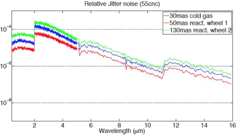
Relative error as function of wavelength for the photon noise limited case (55 Cnc e). Here RPE and residual PDE noise after preliminary de-trending is shown, for three AOCS solutions. Blue: Cold gas system; Red: reaction wheel performance of 50 mas; Green: reaction wheel performance of 130 mas

All sources of instrumental noise contribute to the total system noise level, σ SN. The system noise level is then given by the sum in quadrature of all individual noise components:
σ RO is the detector readout noise, σ DC is the dark current noise, σ Tel is the combined photon noise associated to the thermal emission of all optical surfaces in the line of sight, σ Opt is the photon noise associated to the thermal emission of the module enclosure, and σ RPE+PDE expresses the photometric noise associated to the pointing jitter.
6.2 Simulation of EChO performance
EChOSim simulations were used to estimate the contribution each noise source makes to the total noise budget according to the design of the instrument. The estimated photon noise from the astrophysical scene is used to express the requirement on the excess system noise: this requirement is expressed as:
Where \( {\sigma}_{SN}^R \) is the maximum system noise allowed by the requirement. The parameter X is the excess noise-variance and it is set to X = 2 at wavelengths λ <1 μm, and X = 0.3 at longer wavelengths.
For each noise source contributing to \( {\sigma}_{SN} \), we estimate its contribution to the excess noise-variance, X. For instance, if \( {\sigma}_{RO} \) is the readout noise, its contribution to the excess noise-variance is:
and similarly for all other components contributing to the system noise. Since this number is independent of the integration time and spectral binning, it provides a convenient quantitative way to break down the noise budget in individual components.
Figures 15 and 16 show the contributions to the system noise-variance for the brightest and faintest targets in the proposed EChO sample (see [9] and [10]). For completeness we repeat the definition of the required faint and bright targets from Puig et al. [9] in table 2. In Figs. 15 and 16, the black solid line is the requirement and the red solid curve is the value of X achieved combining all noise sources from simulations. The detector noise is evaluated assuming that the detectors are read “sampling-up-the-ramp”, with 12 non-destructive readings for the bright source case (Fig. 15) and 30 for the faint source case (Fig. 16). The performance evaluation process includes a data reduction pipeline that allows reducing detector timelines into calibrated spectra with removal of the expected systematics [20]. It includes a procedure to remove the jitter noise discussed above and shown in Fig. 14 these errors are strongly correlated with line of sight direction monitored by the FGS. Overall we find that, in the two extreme cases used to set the requirements for the mission design, the systematic noise is less than the requirement over the entire wavelength range. In the faint source case the detector dark current is the largest contributor to systematic noise budget whilst in the bright source case all systematic noise sources are all small compared to the requirement. In the latter case the total noise will be completely dominated by the photon noise from the star, in the faint case the detector performance will be critical to achieving the required performance. In no case were the other potential sources of systematic disturbance, thermal emission, pointing jitter etc., found to produce significant problems.

Noise breakdown for the brightest target proposed to be observed by EChO. The individusal noise components are as follows: readout noise excess variance (dashed green); dark current excess variance dashed blue); thermal emission from instrument enclosures excess variance (dashed violet); thermal mission from optical surfaces excess variance (dashed yellow); post-processing RPE + PDE photometric excess variance (dashed grey). The total variance is shown as the solid red curve and the requirement as the solid black line

Noise breakdown for the faintest target proposed to be observed by EChO. The individual noise components are as detailed in the caption for Fig. 15. The total variance is shown as the solid red curve and the requirement as the solid black line
7 Summary and conclusions
The future of exoplanet research requires that we move from the discovery phase to an investigation of the true nature of the objects through an understanding of the chemistry and physics of their atmospheres, assuming that most exoplanets have one. A dedicated infrared space mission is seen as the most effective way to undertake a survey of a large number of targets plus provide the detailed follow up of a sub-sample of the brightest: the EChO mission proposal was based on this premise. In such a mission the photometric stability is of paramount importance and to this end the spacecraft and payload must be designed as an integrated system. In this paper we have reported on our extensive study into the design and performance of an integrated payload for EChO optimised for the observation of spectra from transiting exoplanets. We find that an instrument based on spectral division using dichroics can provide wavelength coverage from at least 0.4 to 11 μm using detector technology with a high technical readiness level and with only modest requirements on cryogenic cooling – i.e. within the constraints of the ESA medium mission envelope. The instrument design is capable of covering out to 16 μm, albeit using detectors with lower technical readiness and requiring a more aggressive cryogenic design. The instrument design is compact and optimized for high stability spectrophotometric measurements. In particular the fine guidance sensor for the spacecraft pointing shares the same optical path as the science channels and the slitless design of the spectrometers allows for monitoring of the non-target background radiation and, using dark pixels, the dark current of the detectors. The simultaneous measurement of a wide wavelength range ensures that any correlated noise sources can be tracked and accounted for in the data processing. This allows, for instance, the effects of stellar variability to be accounted for and minimised in the data processing as well as any other sources of correlated systematic noise. A comprehensive simulation of the performance of the EChO mission design has been performed which shows that the system would have been limited only by the photon noise from the star for all the targets in the EChO core survey. EChO was not selected for the ESA M3 slot, however the design study has demonstrated that a similar mission is viable and provides a realistic option for furthering exoplanet research. Further progress in detector performance and the reliability of cryogenic system for space applications will mean any future mission will have even better capabilities.
References
Charbonneau, D., et al.: Detection of an Extrasolar Planet Atmosphere”. The Astrophysical Journal Letters 568(377) (2002)
Knutson, H.A., et al.: A Map of the Day-Night Contrast of the Extrasolar Planet HD 189733b”. Nature 447(183) (2007)
Swain, M.R., Vasisht, G., Tinetti, G.: The Presence of Methane in the Atmosphere of an Extrasolar Planet”. Nature 452(329) (2008)
Snellen, I., et al.: The Orbital Motion, Absolute Mass and High-Altitude Winds of Exoplanet HD209458b”. Nature 465(1049) (2010)
Majeau, C., et al.: Two-Dimensional Infrared Map of the Extrasolar Planet HD 189733b”. The Astrophysical Journal Letters 747(20) (2012)
McBride, J., et al.: Experimental Design for the Gemini Planet Imager”. PASP 123, 692–708 (2011)
Fridlund, A.V.M., “The DARWIN project - An ESA cornerstone candidate mission “Planetary Systems in the Universe, Proceedings of IAU Symposium #202, held 7–11 August 2000 at Manchester, United Kingdom. Edited by A. Penny, p451, (2004).
Koch, D.G., et al.: Kepler Mission Design, Realized Photometric Performance, and Early Science”. The Astrophysical Journal Letters 713(79) (2010)
Puig, L., et al., “The Phase 0/A Study of the ESA M3 Mission Candidate EChO” Submitted Exp. A., (2014).
EChO Assessment Study Report, ESA publication ESA/SRE (2013) 2, available at http://sci.esa.int/echo/ accessed 21 July 2014 (2013)
Loose, M., et al.: High-Performance Focal Plane Arrays Based on the HAWAII-2RG/4RG and the SIDECAR ASIC”. Proc. of SPIE 6690(66900C) (2007)
Baker, I., et al., “Mercury Cadmium Telluride Focal Plane Array Developments at Selex ES for Astronomy and Spectroscopy” Proc. of SPIE, 9070, (2014).
McMurtry, C., et al.: “Development of Sensitive Long-Wave Infrared Detector Arrays for Passively Cooled Space Missions”. Optical Engineering 52(9), 091804 (2013)
Lieve, “Accuracy performance of star trackers”, IEEE Trans Aerospace and Electronics Systems, (2002)
Adriani, A., et al., “The Visible and Near Infrared Module of EChO” Submitted Exp A., (2014).
Ramos Zapata, G., et al., “Exoplanet Atmospheres Characterization Observatory Payload Sort-Wave InfraRed Channel: EChO SWiR” Proc. of SPIE, 9143, (2014)
Reess, J.M., et al., “The Mid-Infrared Channel of the EChO Mission” Proc. of SPIE, 9143, (2014).
Bowles, N., et al., “The Long Wavelength Channel of the EChO Mission” submitted to Exp A., (2014).
Bradshaw, T. W. & Orlowska, A. H. “Technology developments on the 4 K cooling system for 'Planck' and FIRST”, Sixth European Symposium on Space Environmental Control Systems, held in Noordwijk, The Netherlands, 20–22 May, 1997. T.-D. Guyenne eds. European Space Agency, SP-400, p.465 (1997)
Waldmann, I., Pascale, E.: “Data analysis Pipeline for EChO end-to-end simulations” arXiv,1402,4408. (2014)
EChO Science Requirements Document, SRE-PA/2011.037; Issue 3, available at http://sci.esa.int/echo/ accessed 21 July 2014 (2013)
EChO Science Requirements Document, SRE-PA/2011.038; Issue 3, available at http://sci.esa.int/echo/ accessed 21 July 2014 (2013)
Author information
Authors and Affiliations
Corresponding author
Rights and permissions
Open Access This article is distributed under the terms of the Creative Commons Attribution License which permits any use, distribution, and reproduction in any medium, provided the original author(s) and the source are credited.
About this article

Cite this article
Eccleston, P., Swinyard, B., Tessenyi, M. et al. The EChO payload instrument – an overview. Exp Astron 40, 427–447 (2015). https://doi.org/10.1007/s10686-014-9428-8
Received:
Accepted:
Published:
Issue Date:
DOI: https://doi.org/10.1007/s10686-014-9428-8