Detectability of labeled weighted automata over monoids

Abstract

In this paper, by developing appropriate methods, we for the first time obtain characterization of four fundamental notions of detectability for general labeled weighted automata over monoids (denoted by $\mathcal {A}^{\mathfrak {M}}$ for short), where the four notions are strong (periodic) detectability (SD and SPD) and weak (periodic) detectability (WD and WPD). The contributions of the current paper are as follows. Firstly, we formulate the notions of concurrent composition, observer, and detector for $\mathcal {A}^{\mathfrak {M}}$. Secondly, we use the concurrent composition to give a necessary and sufficient condition for SD, use the detector to give a necessary and sufficient condition for SPD, and use the observer to give necessary and sufficient conditions for WD and WPD, all for general $\mathcal {A}^{\mathfrak {M}}$ without any assumption. Thirdly, we prove that for a labeled weighted automaton over monoid $(\mathbb {Q}^{k},+)$ (denoted by $\mathcal {A}^{\mathbb {Q}^{k}}$), its concurrent composition, observer, and detector can be computed in NP, 2-EXPTIME, and 2-EXPTIME, respectively, by developing novel connections between $\mathcal {A}^{\mathbb {Q}^{k}}$ and the NP-complete exact path length problem (proven by [Nykänen and Ukkonen, 2002]) and a subclass of Presburger arithmetic. As a result, we prove that for $\mathcal {A}^{\mathbb {Q}^{k}}$, SD can be verified in coNP, while SPD, WD, and WPD can be verified in 2-EXPTIME. Particularly, for $\mathcal {A}^{\mathbb {Q}^{k}}$ in which from every state, a distinct state can be reached through some unobservable, instantaneous path, detector $\mathcal {A}^{\mathbb {Q}^{k}}_{det}$ can be computed in NP, and SPD can be verified in coNP. Finally, we prove that the problems of verifying SD and SPD of deterministic, deadlock-free, and divergence-free $\mathcal {A}^{\mathbb {N}}$ over monoid $(\mathbb {N},+)$ are both coNP-hard. The original methods developed in this paper will provide foundations for characterizing other fundamental properties (e.g., diagnosability and opacity) in labeled weighted automata over monoids. In addition, in order to differentiate labeled weighted automata over monoids from labeled timed automata, we also initially explore detectability in labeled timed automata, and prove that the SD verification problem is PSPACE-complete, while WD and WPD are undecidable.

1 Introduction

1.1 Background and motivation

The state detection problem of partially-observed (aka labeled) dynamical systems has been a fundamental problem in both computer science (Moore 1956) and control science (Kalman 1963) since the 1950s and the 1960s, respectively. Detectability is a basic property of labeled dynamical systems: when it holds one can use an observed label/output sequence generated by a system to reconstruct its current state (Giua and Seatzu 2002; Shu et al. 2007; Sandberg 2005; Zhang et al. 2016). This property plays a fundamental role in many related control problems such as observer design and controller synthesis. Hence in different application scenarios, it is meaningful to characterize different notions of detectability. On the other hand, detectability is strongly related to another fundamental property of diagnosability where the latter describes whether one can use an observed output sequence to determine whether some special events (called faulty events) have occurred (Sampath et al. 1995; Hadjicostis 2020). Recently, a decentralized setting of strong detectability and diagnosability (together with another property called predictability) were unified into one mathematical framework in labeled finite-state automata (Zhang 2021a). Moreover, detectability is also related to several cyber-security properties, e.g., the property of opacity that was originally proposed to describe information flow security in computer science in the early 2000s (Mazaré 2004) can be seen as the absence of detectability.

Discrete-event systems (DESs) are usually composed of transitions between discrete states caused by spontaneous occurrences of labeled events (Wonham and Cai 2019; Cassandras and Lafortune 2010). For DESs modeled by labeled finite-state automata and labeled Petri nets, the detectability problem has been widely studied, see related results on labeled finite-state automata (Shu et al. 2007; Shu and Lin 2011; Zhang 2017; Zhang and Giua 2019; Masopust 2018), and also see related results on labeled Petri nets (Zhang and Giua 2018; Masopust and Yin 2019; Zhang and Giua 2020), and on labeled bounded Petri nets (Lan et al. 2020). Detectability has also been studied for probabilistic finite-state automata (Keroglou and Hadjicostis 2017; Yin 2017).

The above models, either logic systems (labeled finite-state automata and labeled Petri nets), or probabilistic finite-state automata, are untimed. In such models, the time consumption for a transition’s execution is not specified. In spite of this, one can infer from the above literature that all unobservable transitions’ executions are assumed to consume no time by default, and the executions of every pair of observable transitions with the same label are assumed to consume the same time. In order to make these models more realistic, measures to time consumptions for transitions’ executions have been added, so that timed models have been studied, e.g., labeled timed automata¹ (Tripakis 2002; Cassez 2012), special classes of labeled weighted automata over semirings (Lai et al. 2021a; Lai et al. 2021b), etc.

In this paper, we study labeled weighted automata over monoids (Daviaud et al. 2017), denoted by $\mathcal {A}^{\mathfrak {M}}$. Such systems have various features. When monoid $\mathfrak {M}$ is specified as $(\mathbb {Q}_{\geqslant 0},+)$, where $\mathbb {Q}_{\geqslant 0}$ denotes the set of nonnegative rational numbers, $\mathcal {A}^{\mathfrak {M}}$ becomes a one-clock labeled timed automaton in which the clock is reset along with every occurrence of every event and all clock constraints are singletons (details are shown in Section 4) (such automata are exactly the automata studied in (Li et al. 2021)), and hence can represent timed DESs; when $\mathfrak {M}$ is specified as $(\mathbb {Q}^{k},+)$, the weights can represent deviations of positions of a moving object in some region; when $\mathfrak {M}$ is specified as A^∗× B^∗ over alphabets A, B, where A^∗ and B^∗ are free monoids, $\mathcal {A}^{\mathfrak {M}}$ becomes a (finite-state) transducer (Béal and Carton 2002). We will characterize detectability for general $\mathcal {A}^{\mathfrak {M}}$ and will also prove that the results obtained in $\mathcal {A}^{\mathbb {Q}^{k}}$ can be implemented algorithmically. Consider the motivating example as follows.

Example 1

Consider a finite region shown in Fig. 1, in which P₁, P₂, P₃, P₄ denote 4 positions. Assume a robot A walking between these positions to finish a prescribed task. Assume the energy levels of A are quantized into $0,1,\dots ,10$. When A is in position P₁ and moves to P₂, it sends signal a and its target position P₂ along with its energy level decreasing by 1. The other movements can be described analogously, where signal a corresponds to energy level decreasing by 1, signal u corresponds to energy level decreasing by 0 or 1, b corresponds to energy level increasing by 1. A sends a and b, but never sends u. When A sends a signal, it meanwhile sends the corresponding target position. Particularly when the energy level of A is 10 it never increases, i.e., when A is in energy level 10 and moves from P_i to P_i− 1, i = 4,3,2, the energy level of A remains to be 10. Particularly when the energy level of A is 0 it never decreases, i.e., in this case A never moves from P_i to P_i+ 1, i = 1,2,3. All these information is known to a person B. Assume that whenever A sends a or b, B receives/observes the symbols and the corresponding target positions. Then as time advances, B cannot use these observations to determine what the energy level A will be in unless A never moves from P₂ to P₃. For example, assume initially A is in energy level 5 and in position P₁, and assume B knows the initial energy level. When A moves to P₂, B observes a/P₂, and knows that A is in energy level 4. And then A moves to P₃, A could be in energy level 4 or 3 but B does not know A is in P₃. From now on, B will never know what exact energy level A will be in. For example, A moves back to P₂ and could be in energy level 5 or 4, B observes b/P₂; and then A moves to P₃ again, A could be in energy level 5, 4, or 3; and then A moves back to P₂ again, A could be in energy level 6, 5, or 4, B observes b/P₂ (see Table 1). Later in Example 5, we will show this model can be represented by a labeled weighted automaton over some monoid, but cannot be described by a labeled timed automaton.

Fig. 1

The finite region in the motivating Example 1

Table 1 Energy level estimation in the motivating Example 1

1.2 Literature review

Two fundamental definitions are strong detectability and weak detectability (Shu et al. 2007). The former implies that there exists a positive integer k such that for every infinite-length trajectory, each prefix of its label/output sequence of length no less than k allows reconstructing the current state. The latter relaxes the former by changing “every” to “some”. In order to adapt to different application scenarios, variants of strong detectability and weak detectability are also considered, which are called strong periodic detectability (a variant of strong detectability, requiring to determine states periodically along all output sequences) and weak periodic detectability (a variant of weak detectability, requiring to determine states periodically along some output sequence) (Shu et al. 2007). Other essentially different variants of detectability such as eventual strong detectability and weak approximate detectability can be found in Zhang and Giua (2020).

Most results on detectability of labeled finite-state automata are based on two fundamental assumptions of deadlock-freeness (which implies that a system can always run) and divergence-freeness, i.e., having no unobservable cycles (which implies that the running of a system will always be eventually observed). For labeled finite-state automata, under the two assumptions, an observer method (actually the powerset construction used for determinizing nondeterministic finite automata with 𝜖-transitions (Sipser 1996)) was proposed to verify weak (periodic) detectability in exponential time (Shu et al. 2007), later a detector method (a reduced version of the observer, obtained by splitting the states of an observer into subsets of cardinality 2, previously used in (Caines et al. 1988, Caines et al. 1991)) was proposed verify strong (periodic) detectability in polynomial time (Shu and Lin 2011). Also under the two assumptions, verifying weak (periodic) detectability was proven to be PSPACE-complete (Zhang 2017), verifying strong (periodic) detectability was proven to be NL-complete (Masopust 2018). Recently, be developing a concurrent-composition method in Zhang and Giua (2019) and Zhang and Giua (2020) (similar to but technically different from the structures used in (Cassez and Tripakis 2008; Tripakis 2002)), strong detectability was verified in polynomial time without any assumption, removing the two assumptions used for years.

For labeled Petri nets with inhibitor arcs, weak detectability was proven to be undecidable in Zhang and Giua (2018) by reducing the undecidable language equivalence problem of labeled Petri nets (see (Hack 1975)) to negation of weak detectability. For labeled Petri nets, strong detectability was proven to be decidable under the two previously mentioned fundamental assumptions reformulated in labeled Petri nets, it was also proven that it is EXPSPACE-hard to verify strong detectability, but weak detectability is undecidable (Masopust and Yin 2019), which strengthens the related undecidability result proven in Zhang and Giua (2018). In Masopust and Yin (2019), the undecidable language inclusion problem (but not the language equivalence problem) of labeled Petri nets (also see (Hack 1975)) was reduced to negation of weak detectability, so that the same idea in the reduction constructed in Zhang and Giua (2018), i.e., clearing all tokens of the first of the two basic labeled Petri nets, was also implemented. Later, the decidability result for strong detectability was strengthened to hold under only the divergence-freeness assumption (Zhang et al. 2020) by developing a new tool called extended concurrent composition. All decidable results on labeled Petri nets proven by Masopust and Yin (2019) and Zhang et al. (2020) were obtained by reducing negation of strong detectability to satisfiability of some Yen’s path formulae (Yen 1992; Atig and Habermehl 2009).

The notion of observer has been recently extended to a subclass of labeled timed automata in which the automata are deterministic, there is a single clock that is reset along with every occurrence of every event and all clock constraints in all transitions are singletons (Li et al. 2021). This class of labeled timed automata are exactly labeled weighted automata over the monoid $(\mathbb {Q}_{\geqslant 0},+)$, denoted by $\mathcal {A}^{\mathbb {Q}_{\geqslant 0}}$, which are a strict subclass of the automata studied in the current paper. The observer defined in Li et al. (2021) was computed in 2-EXPTIME, and computed in EXPTIME when the considered automata are divergence-free. The method of computing an observer is via unfolding every state q to a finite number n of new states and then compute the observer of the newly obtained labeled finite-state automaton as in Shu et al. (2007), where n is the maximum among the weights of all outgoing transitions of q. Hence the method does not apply to labeled weighted automata with weights being negative rational numbers. In addition, the authors also give an example to show that if some weights are irrational numbers, the observer may have infinitely many states and infinitely many transitions. In Remark 7 of Appendix, we will also use an example in the current paper to illustrate how to compute the observer defined in Li et al. (2021).

The notion of observer has also been extended to subclasses of labeled max-plus automata over the semiring $\underline {\mathbb {Q}}:=(\mathbb {Q}\cup \{-\infty \},\max \limits ,+,-\infty ,0)$, denoted by $\mathcal {A}^{\underline {\mathbb {Q}}}$. In Lai et al. (2021a), the observer was computed for a divergence-free $\mathcal {A}^{unam,\underline {\mathbb {Q}}}$ ($\mathcal {A}^{unam,\underline {\mathbb {Q}}}$ is short for an unambiguous $\mathcal {A}^{\underline {\mathbb {Q}}}$) in EXPTIME, and in Lai et al. (2021b) the observer was computed for a divergence-free, polynomially ambiguous $\mathcal {A}^{\underline {\mathbb {Q}}}$ with the clones property but no upper bound for time complexity was given. In Lai et al. (2021a), the above mentioned four notions of detectability of divergence-free $\mathcal {A}^{unam,\underline {\mathbb {Q}}}$ were verified in EXPTIME by using the observer. In Lai et al. (2021a, 2021b), the authors adopted the max-plus manner to define detectability but not the real-time manner adopted in Li et al. (2021) and the current paper. The detectability results in untimed models mentioned above (e.g., Shu et al. (2007), Zhang (2017), Masopust (2018), Masopust and Yin (2019), and Zhang and Giua (2020)) are all in the real-time manner. Consider a sequence $q_{0}\xrightarrow []{e_{1}}\cdots \xrightarrow []{e_{n}}q_{n}$ of transitions (called a path), where q_i, $0\leqslant i\leqslant n$, are states, e_j, $1\leqslant j\leqslant n$, are events; in the real-time manner, the timed word of the path is $(e_{1},t_{1})\dots (e_{n},t_{n})$, where t_j is the instant when e_j occurs in the path; while in the max-plus manner, the timed sequence of the path is $(e_{1},t_{1}^{\prime })\dots (e_{n},t_{n}^{\prime })$, $t_{j}^{\prime }$ is the maximal time for $e_{1},\dots ,e_{j}$ to occur among all different paths having $e_{1}{\dots } e_{j}$ as their event sequence and having q_j as the final state, so $t_{j}^{\prime }\geqslant t_{j}$. A detailed comparison will be given in Remark of 8 Appendix. The overlaps between the results in Lai et al. (2021b) and the results in the current paper are the results of Lai et al. (2021a), because in $\mathcal {A}^{unam,\underline {\mathbb {Q}}}$, under every event sequence, there exists at most one path from the initial states to any given state, resulting in that the max-plus manner coincides with the real-time manner. The overlaps between the results in Lai et al. (2021b) and the results in Li et al. (2021) are a strict subset of the results in Lai et al. (2021a), i.e., the observer of a divergence-free $\mathcal {A}^{unam,\underline {\mathbb {Q}_{\geqslant 0}}}$ ($\mathcal {A}^{unam,\underline {\mathbb {Q}_{\geqslant 0}}}$ is short for a labeled unambiguous weighted automaton over the semiring $\underline {\mathbb {Q}_{\geqslant 0}}:=(\mathbb {Q}_{\geqslant 0}\cup \{-\infty \},\max \limits ,+,-\infty ,0)$). The relations of the results in Lai et al. (2021a, 2021b) and Li et al. (2021) and the current paper are shown in Fig. 2.

Fig. 2

Relations of the results in Lai et al. (2021a, 2021b) and Li et al. (2021) and the current paper, where Lai et al. (2021a) = C ∪ D (i.e., the results in Lai et al. (2021a) are represented by C ∪ D, the following equalities have similar meanings), Lai et al. (2021b) = A ∪ C ∪ D, Li et al. (2021) = D ∪ E, the current paper= B ∪ C ∪ D ∪ E. The automata considered in A ∪ C ∪ D are divergence-free, the automata considered in E ∪ B are not divergence-free

The results in Lai et al. (2021a) generally do not apply to an automaton $\mathcal {A}^{unam,\underline {\mathbb {Q}}}$ that is not divergence-free (see Remark 9 of Appendix). Although the observer is computed for a general automaton $\mathcal {A}^{\mathbb {Q}_{\geqslant 0}}$ in Li et al. (2021), the observer cannot always be used for verifying detectability for an automaton $\mathcal {A}^{\mathbb {Q}_{\geqslant 0}}$ that is not divergence-free; this is even true in labeled finite-state automata (Zhang and Giua 2020, Remark 2). Detectability of general $\mathcal {A}^{unam,\underline {\mathbb {Q}}}$ and general $\mathcal {A}^{\mathbb {Q}_{\geqslant 0}}$ can be verified by using the methods developed in the current paper, for the first time. Apart from the above advantages of the current paper compared with Li et al. (2021) and Lai et al. (2021a), we also show that $\mathcal {A}^{unam,\underline {\mathbb {N}}}$ and $\mathcal {A}^{unam,\mathbb {N}}$ are already fundamentally more complicated than a labeled finite-state automaton $\mathcal {A}$ by proving in Theorem 14 that, the problems of verifying strong (periodic) detectability of deterministic, deadlock-free, and divergence-free $\mathcal {A}^{unam,\underline {\mathbb {N}}}$ and $\mathcal {A}^{unam,\mathbb {N}}$ are coNP-hard, where $\mathcal {A}^{unam,\underline {\mathbb {N}}}$ denotes a labeled unambiguous weighted automaton over the max-plus semiring $\underline {\mathbb {N}}:=(\mathbb {N}\cup \{-\infty \},\max \limits ,+,-\infty ,0)$, $\mathcal {A}^{unam,\mathbb {N}}$ denotes a labeled unambiguous weighted automaton over monoid $(\mathbb {N},+,0)$, because as previously mentioned, strong (periodic) detectability of automaton $\mathcal {A}$ can be verified in polynomial time (Shu and Lin 2011; Zhang and Giua 2019).

Probabilistic finite-state automata were also widely studied models in DESs (e.g., in Keroglou and Hadjicostis 2017 and Yin 2017). They are actually weighted automata over the semiring $(\mathbb {R},+,\cdot ,0,1)=:\underline {\mathbb {R}}$, but the weights are only chosen from [0,1]. Because only probabilities are computed, no computation produces a value outside [0,1]. In such automata, the reliability of an event sequence is defined as the sum of the reliabilities of its successful paths, where the reliability of a successful path is the product of the probabilities (i.e., weights) of all its transitions. Hence the detectability notions studied in Keroglou and Hadjicostis (2017) and Yin (2017) are defined in a totally different way compared with those in Lai et al. (2021a) and Li et al. (2021) and the current paper. On the other hand, in this paper we will give necessary and sufficient conditions for four fundamental notions of detectability of labeled weighted automata over any monoids, which include the results on labeled weighted automata over the monoid $(\mathbb {R},\cdot ,1)$ as a special sub class.

1.3 Contributions of the paper

The first contribution is on a general labeled weighted automaton over a monoid, denoted by $\mathcal {A}^{\mathfrak {M}}$.

• 1. We for the first time formulate the notions of concurrent composition, observer, and detector for $\mathcal {A}^{\mathfrak {M}}$, which are natural but nontrivial extensions of those for labeled finite-state automata. We use the notion of concurrent composition to give necessary and sufficient condition for strong detectability, use the notion of observer to give necessary and sufficient conditions for weak detectability and weak periodic detectability, and use the notion of detector to give necessary and sufficient condition for strong periodic detectability, all for general $\mathcal {A}^{\mathfrak {M}}$ without any assumption.

The second contribution of the paper is on labeled weighted automata over the monoid $(\mathbb {Q}^{k},+,0_{k})$ (denoted by $\mathcal {A}^{\mathbb {Q}^{k}}$), where $0_{k}\in \mathbb {Q}^{k}$ denotes the k-length zero vector, in which the special results on unambiguous $\mathcal {A}^{\mathbb {Q}}$ also hold for labeled unambiguous weighted automata over semiring $\underline {\mathbb {Q}}$ (denoted by $\mathcal {A}^{unam,{\underline {\mathbb {Q}}}}$), because the four notions of detectability of $\mathcal {A}^{unam,\underline {\mathbb {Q}}}$ in Lai et al. (2021a) coincide with the four notions of detectability of $\mathcal {A}^{unam,\mathbb {Q}}$ in the current paper correspondingly (except for minor and neglectable differences, see Remark 8 of Appendix).

• 2. We find novel connections between $\mathcal {A}^{\mathbb {Q}^{k}}$ and the exact path length problem (Nykänen and Ukkonen 2002) and a subclass of Presburger arithmetic (Grädel 1988) so that detectability of $\mathcal {A}^{\mathbb {Q}^{k}}$ can be verified.

• 3. For $\mathcal {A}^{\mathbb {Q}^{k}}$, we prove that its observer and detector can be computed in 2-EXPTIME, its self-composition can be computed in NP, all in the size of $\mathcal {A}^{\mathbb {Q}^{k}}$.

• 4. We prove that strong detectability of $\mathcal {A}^{\mathbb {Q}^{k}}$ can be verified in coNP, while strong periodic detectability, weak detectability, and weak periodic detectability of $\mathcal {A}^{\mathbb {Q}^{k}}$ can be verified in 2-EXPTIME, all in the size of $\mathcal {A}^{\mathbb {Q}^{k}}$. Particularly for $\mathcal {A}^{\mathbb {Q}^{k}}$ in which from every state, a distinct state can be reached through some unobservable, instantaneous path, its detector can be computed in NP, and its strong periodic detectability can be verified in coNP. We also prove that the problems of verifying strong detectability and strong periodic detectability of deterministic, deadlock-free, and divergence-free $\mathcal {A}^{\mathbb {N}}$ are both coNP-hard. See Tables 2 and 3 as collections of related results.

Table 2 Results on complexity of verifying four notions of detectability of automata, where SD, SPD, WD, and WPD are short for strong detectability, strong periodic detectability, weak detectability, and weak periodic detectability, respectively; $\mathcal {A}$ denotes a labeled finite-state automaton, $\mathcal {A}^{\mathbb {Q}^{k}}$ (resp., $\mathcal {A}^{\underline {\mathbb {Q}}}$, $\mathcal {A}^{\underline {\mathbb {N}}}$, $\mathcal {A}^{\mathbb {N}}$) denotes a labeled weighted automaton over monoid $(\mathbb {Q}^{k},+,0_{k})$ (resp., max-plus semiring $(\mathbb {Q}\cup \{-\infty \},\max \limits ,+,-\infty ,0)$, max-plus semiring $(\mathbb {N}\cup \{-\infty \},\max \limits ,+,-\infty ,0))$, monoid $(\mathbb {N},+,0))$, “u.” is short for “unambiguous”, “d.d.” is short for “deadlock-free, divergence-free”, “d.d.d” is short for “deterministic, deadlock-free, divergence-free”, “c.” denotes “complete”, “h.” denotes “hard”

Table 3 Results on complexity of computing observers, detectors, and self-compositions of automata, where $\mathcal {A}$, $\mathcal {A}^{\mathbb {Q}^{k}}$, $\mathcal {A}^{\underline {\mathbb {Q}}}$, u. are the same as those in Table 2, $\mathcal {A}^{\mathbb {Q}_{\geqslant 0}}$ denotes a labeled weighted automaton over the monoid $(\mathbb {Q}_{\geqslant 0},+,0)$, “d.” is short for “divergence-free”

Finally, in order to differentiate labeled weighted automata over monoids from labeled timed automata, we also initially explore detectability in labeled timed automata.

• 5. We prove that in labeled timed automata, the strong detectability verification problem is PSPACE-complete, while weak (periodic) detectability is undecidable.

2 Preliminaries

2.1 Notation

Symbols $\mathbb {N}$, $\mathbb {Z}$, $\mathbb {Z}_{+}$, $\mathbb {Q}$, $\mathbb {Q}_{\geqslant 0}$, $\mathbb {R}$, and $\mathbb {R}_{\geqslant 0}$ denote the sets of nonnegative integers, integers, positive integers, rational numbers, nonnegative rational numbers, real numbers, and nonnegative real numbers, respectively. Symbol 0_k denotes the k-length zero vector. For a finite alphabet Σ, Σ^∗ and Σ^ω are used to denote the set of words (i.e., finite-length sequences of elements of Σ) over Σ including the empty word 𝜖 and the set of configurations (i.e., infinite-length sequences of elements of Σ) over Σ, respectively. Σ⁺ := Σ^∗∖{𝜖}. For a word s ∈Σ^∗, |s| stands for its length, and we set $|s^{\prime }|=+\infty$ for all $s^{\prime }\in {\varSigma }^{\omega }$. For s ∈Σ⁺ and $k\in \mathbb {N}$, s^k and s^ω denote the concatenations of k copies of s and infinitely many copies of s, respectively. Analogously, L₁L₂ := {e₁e₂|e₁ ∈ L₁, e₂ ∈ L₂}, where $L_{1},L_{2}\subset {\varSigma }^{*}$. For a word (configuration) s ∈Σ^∗(Σ^ω), a word $s^{\prime }\in {\varSigma }^{*}$ is called a prefix of s, denoted as $s^{\prime }\sqsubset s$, if there exists another word (configuration) $s^{\prime \prime }\in {\varSigma }^{*}({\varSigma }^{\omega })$ such that $s=s^{\prime }s^{\prime \prime }$. For two nonnegative integers $i\leqslant j$, [[i, j]] denotes the set of all integers no less than i and no greater than j; and for a set S, |S| denotes its cardinality and 2^S its power set. Symbols ⊂ and $\subsetneq$ denote the subset and strict subset relations, respectively.

We will use the exact path length (EPL) problem, the subset sum problem, and a subclass of Presburger arithmetic in the literature to prove the main results.

2.2 The exact path length problem

Consider a k-dimensional weighted directed graph $G=(\mathbb {Q}^{k},V,A)$, where $k\in \mathbb {Z}_{+}$, $\mathbb {Q}^{k}=\underbrace {\mathbb {Q}\times \cdots \times \mathbb {Q}}_{k}$, V is a finite set of vertices, $A\subset V\times \mathbb {Q}^{k}\times V$ a finite set of weighted edges (arcs) with weights in $\mathbb {Q}^{k}$. For a path $v_{1}\xrightarrow []{z_{1}}\cdots \xrightarrow []{z_{n-1}}v_{n}$, its weight is defined by ${\sum }_{i=1}^{n-1}z_{i}$. For an edge a = (v₁, z, v₂) ∈ A, also denoted by $v_{1}\xrightarrow [] {z}v_{2}$, we call v₁ and v₂ the tail (denoted by tail(a)) and the head (denoted by head(a)) of a, respectively. The EPL problem (Nykänen and Ukkonen 2002) is stated as follows.

Problem 1 (EPL)

Given a positive integer k, a k-dimensional weighted directed graph $G=(\mathbb {Q}^{k},V,A)$, two vertices v₁, v₂ ∈ V, and a vector $z\in \mathbb {Q}^{k}$, determine whether there exists a path from v₁ to v₂ with weight z.

We set as usual that for a positive integer n, the size size(n) of n to be the length of its binary representation, i.e., $size(n)=\lceil {\log _{2}{(n+1)}}\rceil$ (⌈⋅⌉ is the ceiling function), size(−n) = 1 + size(n); size(0) = 1; for a rational number m/n, where m, n are relatively prime integers, size(m/n) = size(m) + size(n); then for a vector $z\in \mathbb {Q}^{k}$, its size is the sum of the sizes of its entries. The size of an instance (k, G, v₁, v₂, z) of the EPL problem is defined by size(k) + size(G) + 2 + size(z), where size(G) = |V | + size(A), $size(A)={\sum }_{(v_{1},z^{\prime },v_{2})\in A} (2+size(z^{\prime }))$.

Lemma 1 (Nykänen and Ukkonen 2002)

The EPL problem belongs to NP.² The EPL problem is NP-hard already for graph $(\mathbb {N},V,A)$.

2.3 The subset sum problem

The subset sum problem (Garey and Johnson 1990, p. 223) is as follows.

Problem 2 (subset sum)

Given positive integers $n_{1},\dots ,n_{m}$, and N, determine whether $N={\sum }_{i\in I}n_{i}$ for some I ⊂ [[1, m]].

Lemma 2 (Garey and Johnson 1990)

The subset sum problem is NP-complete.

2.4 Presburger arithmetic

We will use a subclass of Presburger arithmetic. A Presburger formula/sentence of this subclass is as follows:

$$ \begin{array}{@{}rcl@{}} (Q_{1} x_{1}\in\mathbb{N})\dots(Q_{s} x_{s}\in\mathbb{N})[{\Phi}(x_{1},\dots,x_{s})], \end{array} $$

(1)

where $Q_{1},\dots ,Q_{s}$ are any quantifier prefix (Q_i = ∃ (existential quantifier) or ∀ (universal quantifier)), $x_{1},\dots ,x_{s}$ are variables, ${\Phi }(x_{1},\dots ,x_{s})$ is a formula consisting of a Boolean combination of linear inequalities of the form

$$ \begin{array}{@{}rcl@{}} a_{1}x_{1}+\cdots+a_{s}x_{s} \leqslant b \end{array} $$

(2)

with $a_{1},\dots ,s_{s},b$ constant integers.

For example, $(x_{1}=1)=(x_{1}\geqslant 1)\wedge (x_{1}\leqslant 1)=\neg (x_{1}\leqslant 1)\wedge (x_{1}\leqslant 1)$ and $(x_{1}=1)\implies (x_{2}>2)=\neg (x_{1}=1) \vee \neg (x_{2}\leqslant 2)$ are such quantifier-free formulae.

Lemma 3 (Grädel 1988)

Consider a Presburger sentence as in Eq. 1 of length r with m quantifier alternations (i.e., with m blocks of adjacent quantifiers of the same kind). Then the sentence is satisfied if and only if

$$(Q_{1} x_{1}\leqslant w)\dots(Q_{s} x_{s}\leqslant w) [{\Phi}(x_{1},\dots,x_{s})]$$

is satisfied, where $w=2^{cr^{(s+3)^{m+1}}}$, c is a constant.

This yields a decision procedure: one can first compute w from r, m, s, and then check all s-tuples of nonnegative integers $x_{1},\dots ,x_{s}$ with $x_{i}\leqslant w$, whether ${\Phi }(x_{1},\dots ,x_{s})$ is true.

In Eq. 1, if $s\in \mathbb {Z}_{+}$ is also regarded as input, Q₁ = ⋯ = Q_s = ∃, and ${\Phi }(x_{1},\dots ,x_{s})$ is conjunctions of linear equations of the form a₁x₁ + ⋯ + a_sx_s = b with $a_{1},\dots ,a_{s},b$ constant rational numbers, then Eq. 1 becomes the NP-complete integer linear programming (Papadimitriou 1981; Schrijver 1986).

2.5 Labeled weighted automata over monoids

A monoid is a triple $\mathfrak {M}=(T,\otimes ,{\textbf {1}})$, where for all a, b, c ∈ T,

• a ⊗ b ∈ T,

• (associativity) (a ⊗ b) ⊗ c = a ⊗ (b ⊗ c),

• a ⊗1 = 1 ⊗ a = a (1 ∈ T is called identity of $\mathfrak {M}$).

Particularly, if there exists an element 0 ∈ T such that 0 ⊗ a = a ⊗0 = 0 for all a ∈ T, then we call 0 zero of $\mathfrak {M}$. Any monoid has exactly one identity and at most one zero.

A labeled weighted automaton over monoid $\mathfrak {M}=(T,\otimes ,{\textbf 1})$ is a tuple

$$ \begin{array}{@{}rcl@{}} \mathcal{A}^{\mathfrak{M}}=(\mathfrak{M},Q,E,Q_{0},{\varDelta},\alpha,\mu,{\varSigma},\ell), \end{array} $$

(3)

where Q is a finite set of states, E a finite alphabet (elements of E are called events), Q₀ ⊂ Q a set of initial states, Δ ⊂ Q × E × Q a transition relation (elements of Δ are called transitions, a transition $(q,e,q^{\prime })\in {\varDelta }$ is interpreted as when $\mathcal {A}^{\mathfrak {M}}$ is in state q and event e occurs, $\mathcal {A}^{\mathfrak {M}}$ transitions to state $q^{\prime }$), α assigns to each initial state q₀ ∈ Q₀ a nonzero weight α(q₀) ∈ T, μ assigns to each transition $(q,e,q^{\prime })\in {\varDelta }$ (or rewritten as $q\xrightarrow []{e}q^{\prime }$) a nonzero weight$\mu (e)_{qq^{\prime }}\in T$, where the transition is also denoted by $q\xrightarrow []{e/\mu (e)_{qq^{\prime }}}q^{\prime }$, Σ is a finite set of outputs/labels, and ℓ : E →Σ∪{𝜖} is a labeling function.

Particularly, $\mathcal {A}^{\mathbb {Q}^{k}}$, $\mathcal {A}^{\mathbb {Q}_{\geqslant 0}}$, $\mathcal {A}^{\mathbb {N}}$ denote $\mathcal {A}^{\mathfrak {M}}$ in which $\mathfrak {M}$ is specified as $(\mathbb {Q}^{k},+,0_{k})$, $(\mathbb {Q}_{\geqslant 0},+,0)$, $(\mathbb {N},+,0)$, where $\mathcal {A}^{\mathbb {Q}_{\geqslant 0}}$ and $\mathcal {A}^{\mathbb {N}}$ can represent timed DESs. The size $size(\mathcal {A}^{\mathbb {Q}^{k}})$ of a given $\mathcal {A}^{\mathbb {Q}^{k}}$ is defined by |Q| + |Δ| + size(α) + size(μ) + size(ℓ), where the size of a rational vector has already been defined before, $size(\alpha )=|Q_{0}|+{\sum }_{q\in Q_{0}}size(\alpha (q))$, $size(\mu )={\sum }_{(q,e,q^{\prime })\in {\varDelta }} size(\mu (e)_{qq^{\prime }})$, size(ℓ) = |{(e, ℓ(e))|e ∈ E}|. The size of a given $\mathcal {A}^{\mathbb {Q}_{\geqslant 0}}$ (resp., $\mathcal {A}^{\mathbb {N}}$) can be defined analogously.

Remark 1

A labeled finite-state automaton (studied in Shu et al. 2007, Shu and Lin 2011, Masopust 2018, Zhang 2017, etc.) can be regarded as automaton $\mathcal {A}^{\mathbb {N}}$ such that all unobservable transitions are instantaneous and every two observable transitions with the same label have the same weight in $\mathbb {N}$. The observer of such $\mathcal {A}^{\mathbb {N}}$ can be computed in exponential time (Shu et al. 2007). In the sequel, we use $\mathcal {A}$ to denote a labeled finite-state automaton (without weights).

Events in E_uo = {e ∈ E|ℓ(e) = 𝜖} are called unobservable, events in E_o = {e ∈ E|ℓ(e)≠𝜖} are called observable. When an observable event e ∈ E_o occurs, ℓ(e) is observed; but when an unobservable event e ∈ E_uo occurs, nothing is observed. For every q ∈ Q, we also regard $q\xrightarrow []{\epsilon /{\textbf 1}}q$ as a transition. A transition $q\xrightarrow []{e/\mu (e)_{qq^{\prime }}}q^{\prime }$ is called instantaneous if $\mu (e)_{qq^{\prime }} ={\textbf 1}$, and called noninstantaneous otherwise. A transition $q\xrightarrow []{e/\mu (e)_{qq^{\prime }}}q^{\prime }$ is called observable (resp., unobservable) if e is observable (resp., unobservable). We denote by ${\varDelta }_{o}=\{(q,e,q^{\prime })\in {\varDelta }|\ell (e)\ne \epsilon \}$ and ${\varDelta }_{uo}=\{(q,e,q^{\prime })\in {\varDelta }|\ell (e)=\epsilon , e\ne \epsilon \}$ the sets of observable transitions and unobservable transitions, respectively. Particularly, we denote E_a = {e ∈ E_o|ℓ(e) = a}, ${\varDelta }_{a}=\{(q,e,q^{\prime })\in {\varDelta }|\ell (e)=a\}$, where a ∈Σ. Automaton $\mathcal {A}^{\mathfrak {M}}$ is called deterministic if (1) |Q₀| = 1 and (2) for all states $q,q^{\prime },q^{\prime \prime }\in Q$ and events e ∈ E, if $(q,e,q^{\prime })\in {\varDelta }$ and $(q,e,q^{\prime \prime })\in {\varDelta }$ then $q^{\prime }=q^{\prime \prime }$ (hence one also has $\mu (e)_{qq^{\prime }}=\mu (e)_{qq^{\prime \prime }}$).

From now on, without loss of generality, we assume for each initial state q₀ ∈ Q₀, α(q₀) = 1, because otherwise we add a new initial state $q_{0}^{\prime }\notin Q$ and set $\alpha (q_{0}^{\prime })=\textbf {1}$; and then for each initial state q₀ ∈ Q₀ such that α(q₀)≠1, we let q₀ not be initial any more, and add a transition $q_{0}^{\prime }\xrightarrow []{\varepsilon / \alpha (q_{0})} q_{0}$, where ε is a new event not in E and unobservable. The case for $\mathcal {A}^{\mathbb {Q}_{\geqslant 0}}$ is interpreted as follows: if an automaton was initially in state q₀, then before instant α(q₀), no event occurred, hence nothing could be observed. So it makes sense to set ε to be unobservable.

Particularly for $\mathcal {A}^{\mathbb {Q}_{\geqslant 0}}$, for initial state q ∈ Q₀, α(q) denotes its initial time delay, and in a transition $q\xrightarrow []{e/\mu (e)_{qq^{\prime }}}q^{\prime }$, $\mu (e)_{qq^{\prime }}$ denotes its time delay (i.e., the time consumption of its execution). Hence the execution of an instantaneous transition has time delay 0, i.e., does not cost time, while the execution of a noninstantaneous transition has time delay a positive rational number $\mu (e)_{qq^{\prime }}$, i.e., costs time $\mu (e)_{qq^{\prime }}$. As pointed out before, without loss of generality, we assume α(q₀) = 0 for all q₀ ∈ Q₀.

For $q_{0},\dots ,q_{n}\in Q$ and $e_{1},\dots ,e_{n}\in E$, $n\in \mathbb {Z}_{+}$, we call a sequence

$$ \begin{array}{@{}rcl@{}} \pi:=q_{0}\xrightarrow[]{e_{1}}q_{1}\xrightarrow[]{e_{2}}\cdots\xrightarrow[]{e_{n}}q_{n} \end{array} $$

(4)

of transitions a (finite) path. A state q is called reachable if it is initial or there exists a path from some initial state to q. A path π is called simple if $q_{0},\dots ,q_{n}$ are pairwise different. A path π is called a cycle if q₀ = q_n, and a simple cycle is such that $q_{0},\dots ,q_{n-1}$ are pairwise different. A path π is called unobservable if $\ell (e_{1}{\dots } e_{n})=\epsilon$, and called observable otherwise. The set of paths starting at q₀ ∈ Q and ending at q ∈ Q is denoted by . Particularly, for denotes the set of all paths under $e_{1}{\dots } e_{n}$, i.e., the paths $q_{0}\xrightarrow []{e_{1}}q_{1}\xrightarrow []{e_{2}}{\cdots } \xrightarrow []{e_{n-1}}q_{n-1}\xrightarrow []{e_{n}}q$, where $q_{1},\dots ,q_{n-1}\in Q$. Automaton $\mathcal {A}^{\mathfrak {M}}$ is called unambiguous if under every event sequence, there exists at most one path from the initial states to any given state, i.e., for all s ∈ E⁺ and q ∈ Q, one has . If $\mathcal {A}^{\mathfrak {M}}$ is deterministic then it is unambiguous.

The weighted word of path π is defined by

$$ \begin{array}{@{}rcl@{}} \tau(\pi):=(e_{1},t_{1})(e_{2},t_{2})\dots(e_{n},t_{n}), \end{array} $$

(5)

where for all i ∈ [[1, n]], $t_{i}=\bigotimes _{j=1}^{i}\mu (e_{j})_{q_{j-1}q_{j}}$.The weight of path π is defined by t_n =: WT_π. A path π is called instantaneous if t₁ = ⋯ = t_n = 1, and called noninstantaneous otherwise.

Particularly for $\mathcal {A}^{\mathbb {Q}_{\geqslant 0}}$, one has $t_{i}={\sum }_{j=1}^{i}{\mu (e_{j})_{q_{j-1}q_{j}}}$, hence the t_i in τ(π) can be used to denote the total time consumptions for the first i transitions in path π, i ∈ [[1, n]]. Hence we also call a weighted word of automaton $\mathcal {A}^{\mathbb {Q}_{\geqslant 0}}$ timed word. If $\mathcal {A}^{\mathbb {Q}_{\geqslant 0}}$ generates a path π as in Eq. 4, consider its timed word τ(π) as in Eq. 5, then at instant t_i, one observes ℓ(e_i) if ℓ(e_i)≠𝜖; and observes nothing otherwise, where i ∈ [[1, n]]. We simply say one observes ℓ(τ(π)). With this intuitive observation, we will define the notion of current-state estimate in the next section.

We use $L(\mathcal {A}^{\mathfrak {M}})$ to denote the set of weighted words of all paths of $\mathcal {A}^{\mathfrak {M}}$ starting from initial states.

For $q_{0},q_{1},\dots \in Q$ and $e_{1},e_{2},\dots \in E$, we call

$$ \begin{array}{@{}rcl@{}} \pi:=q_{0}\xrightarrow[]{e_{1}}q_{1}\xrightarrow[]{e_{2}}\cdots \end{array} $$

(6)

an infinite path. The ω-weighted word of infinite path π is defined by

$$ \begin{array}{@{}rcl@{}} \tau(\pi):=(e_{1},t_{1})(e_{2},t_{2})\dots, \end{array} $$

(7)

where for all $i\in \mathbb {Z}_{+}$, $t_{i}=\bigotimes _{j=1}^{i}\mu (e_{j})_{q_{j-1}q_{j}}$.

We use $L^{\omega }(\mathcal {A}^{\mathfrak {M}})$ by to denote the set of ω-weighted words of all infinite paths of $\mathcal {A}^{\mathfrak {M}}$ starting from initial states. Particularly, we also call an ω-weighted word of automaton $\mathcal {A}^{\mathbb {Q}_{\geqslant 0}}$ ω-timed word.

Labeling function ℓ is recursively extended to E^∗∪ E^ω →Σ^∗∪Σ^ω as $\ell (e_{1}e_{2}\dots )\\=\ell (e_{1})\ell (e_{2})\dots$. We also extend ℓ as follows: for all (e, t) ∈ E × T, ℓ((e, t)) = (ℓ(e),t) if ℓ(e)≠𝜖, and ℓ((e, t)) = 𝜖 otherwise. Hence ℓ is also recursively extended to (E × T)^∗∪ (E × T)^ω → (Σ × T)^∗∪ (Σ × T)^ω. For a weighted word τ(π), where π is a path of $\mathcal {A}^{\mathfrak {M}}$, ℓ(τ(π)) is called the weighted label/output sequence of both π and τ(π). We also extend the previously defined function τ as follows: for all $\gamma =(\sigma _{1},t_{1})\dots (\sigma _{n},t_{n})\in ({\varSigma }\times T)^{*}$,

$$ \tau(\gamma)=(\sigma_{1},t_{1}^{\prime})\dots(\sigma_{n},t_{n}^{\prime}), $$

(8)

where $t_{j}^{\prime }=\bigotimes _{i=1}^{j}t_{i}$ for all j ∈ [[1, n]]. Moreover, τ is also extended to (Σ × T)^ω recursively.

The weighted language ${\mathscr{L}}(\mathcal {A}^{\mathfrak {M}})$ and ω-weighted language ${\mathscr{L}}^{\omega } (\mathcal {A}^{\mathfrak {M}})$ generated by $\mathcal {A}^{\mathfrak {M}}$ are defined by

$$ \begin{array}{@{}rcl@{}} \mathcal{L}(\mathcal{A}^{\mathfrak{M}}) &:= \{\gamma\in({\varSigma}\times T)^{*}|(\exists w\in L(\mathcal{A}^{\mathfrak{M}}))[\ell(w)=\gamma]\} \end{array} $$

(9)

and

$$ \begin{array}{@{}rcl@{}} \mathcal{L}^{\omega}(\mathcal{A}^{\mathfrak{M}}) &:= \{\gamma\in({\varSigma}\times T)^{\omega}|(\exists w\in L^{\omega}(\mathcal{A}^{\mathfrak{M}}))[\ell(w)=\gamma]\}, \end{array} $$

(10)

respectively. Particularly, we also call ${\mathscr{L}}(\mathcal {A}^{\mathbb {Q}_{\geqslant 0}})$ and ${\mathscr{L}}^{\omega }(\mathcal {A}^{\mathbb {Q}_{\geqslant 0}})$ timed language and ω-timed language, respectively.

Example 2

A labeled unambiguous weighted automaton $\mathcal {A}_{0}^{\underline {\mathbb {N}}}$ over semiring $\underline {\mathbb {N}}$ is shown in Fig. 3. Because $\mathcal {A}_{0}^{\underline {\mathbb {N}}}$ is unambiguous, it is the same as the labeled weighted automaton $\mathcal {A}_{0}^{\mathbb {N}}$ over monoid $(\mathbb {N},+)$,

Fig. 3

Labeled unambiguous weighted automaton $\mathcal {A}_{0}^{\underline {\mathbb {N}}}$ ($\mathcal {A}_{0}^{\mathbb {N}}$) that is not divergence-free, where event u is unobservable (we denote ℓ(u) = 𝜖), event a is observable (we denote ℓ(a) = a)

Example 3

Consider labeled weighted automaton $\mathcal {A}^{\mathbb {N}}_{1}$ shown in Fig. 4, where only q₀ is initial, event u is unobservable, events a and b are observable, ℓ(a) = ℓ(b) = ρ. Automaton $\mathcal {A}_{1}^{\mathbb {N}}$ is ambiguous, because q₃ can be reached from q₀ through two paths $q_{0}\xrightarrow []{a} q_{1}\xrightarrow []{b} q_{3}$ and $q_{0}\xrightarrow []{a} q_{2} \xrightarrow []{b} q_{3}$ under the same event sequence ab.

Consider paths

$$ \begin{array}{@{}rcl@{}} \pi_{1}=q_{0}\xrightarrow[]{a} q_{1}\xrightarrow[]{b} q_{3}, && \quad \pi_{2}=q_{0}\xrightarrow[]{a} q_{2}\xrightarrow[]{b} q_{3}, \end{array} $$

(11a)

$$ \begin{array}{@{}rcl@{}} \pi_{3}=q_{0}\xrightarrow[]{a} q_{1}\xrightarrow[]{u} q_{1}\xrightarrow[]{b} q_{3}, && \quad \pi_{4}=q_{0}\xrightarrow[]{a} q_{2}\xrightarrow[]{u} q_{2}\xrightarrow[]{b} q_{3}, \end{array} $$

(11b)

$$ \begin{array}{@{}rcl@{}} \pi_{5}=q_{0}\xrightarrow[]{a} q_{2}\xrightarrow[]{b} q_{3}\xrightarrow[]{u} q_{4}, && \end{array} $$

(11c)

one then has

$$ \begin{array}{@{}rcl@{}} \tau(\pi_{1})=(a,1)(b,3), && \quad \ell(\tau(\pi_{1}))=(\rho,1)(\rho,3), \end{array} $$

(12a)

$$ \begin{array}{@{}rcl@{}} \tau(\pi_{2})=(a,1)(b,2), && \quad \ell(\tau(\pi_{2}))=(\rho,1)(\rho,2), \end{array} $$

(12b)

$$ \begin{array}{@{}rcl@{}} \tau(\pi_{3})=(a,1)(u,2)(b,4), && \quad \ell(\tau(\pi_{3}))=(\rho,1)(\rho,4), \end{array} $$

(12c)

$$ \begin{array}{@{}rcl@{}} \tau(\pi_{4})=(a,1)(u,2)(b,3), && \quad \ell(\tau(\pi_{4}))=(\rho,1)(\rho,3), \end{array} $$

(12d)

$$ \begin{array}{@{}rcl@{}} \tau(\pi_{5})=(a,1)(b,2)(u,3), && \quad \ell(\tau(\pi_{5}))=(\rho,1)(\rho,2). \end{array} $$

(12e)

Fig. 4

Labeled ambiguous weighted automaton $\mathcal {A}_{1}^{\mathbb {N}}$, where ℓ(u) = 𝜖, ℓ(a) = ℓ(b) = ρ

Path π₁ has the following meaning: $\mathcal {A}_{1}^{\mathbb {N}}$ starts at initial state q₀; when event a occurs after time segment 1, $\mathcal {A}_{1}^{\mathbb {N}}$ transitions to state q₁, we observe ρ at time instant 1; when event b occurs after time segment 2 since the occurrence of the previous event a, $\mathcal {A}_{1}^{\mathbb {N}}$ transitions to state q₃, and we observe ρ at time instant 3. The other paths have similar interpretations.

3 Main results

3.1 The definition of current-state estimate

For automaton $\mathcal {A}^{\mathfrak {M}}$, for 𝜖, we define the instantaneous initial-state estimate by

(13)

Analogously, for a subset x ⊂ Q, we define its instantaneous-state estimate by

(14)

${\mathscr{M}}(\mathcal {A}^{\mathfrak {M}},\epsilon )$ denotes the set of states $\mathcal {A}^{\mathfrak {M}}$ can be in at the initial time before any possible observable event occurs (note that an observable event may occur at the initial time when the event is in some instantaneous transition starting from some initial state), so we only consider unobservable, instantaneous paths, which is represented by τ(π) ∈ (E_uo ×{1})⁺.

More generally, for $\mathcal {A}^{\mathfrak {M}}$, for weighted label/output sequence γ ∈ (Σ × T)⁺, we define the current-state estimate as

$$ \begin{array}{@{}rcl@{}} \mathcal{M}(\mathcal{A}^{\mathfrak{M}},\gamma):=\{q\in Q|&& \!\!\!\!\!(\exists\text{ a path }q_{0}\xrightarrow[]{s^{\prime}}q^{\prime}\xrightarrow[]{s}q)[\\ &&\!\!\!\!\!(q_{0}\in Q_{0})\wedge(s^{\prime}\in E^{*}E_{o})\wedge(s\in(E_{uo})^{*})\wedge\\ &&\!\!\!\!\!(\ell(\tau(q_{0}\xrightarrow[]{s^{\prime}}q^{\prime}))=\gamma)\wedge (\tau(q^{\prime}\xrightarrow[]{s}q)\in(E_{uo}\times\{{\textbf1}\})^{*})]\}. \end{array} $$

(15)

Intuitively, for $\gamma =(\sigma _{1},t_{1})\dots (\sigma _{n},t_{n})\in ({\varSigma }\times T)^{+}$, ${\mathscr{M}}(\mathcal {A}^{\mathfrak {M}},\gamma )$ denotes the set of states $\mathcal {A}^{\mathfrak {M}}$ can be in when γ has just been generated by $\mathcal {A}^{\mathfrak {M}}$. Particularly for $\mathcal {A}^{\mathbb {Q}_{\geqslant 0}}$, ${\mathscr{M}}(\mathcal {A}^{\mathbb {Q}_{\geqslant 0}},\gamma )$ denotes the set of states $\mathcal {A}^{\mathbb {Q}_{\geqslant 0}}$ can be in when we just observe $\gamma \in ({\varSigma }\times \mathbb {Q}_{\geqslant 0})^{*}$. In order to fit the setting of current-state estimate, after the occurrence of the last observable event (denoted by e_o) in $s^{\prime }$ (i.e., e_o occurs at the current time), we only allow unobservable, instantaneous paths, which is represented by $\tau (q^{\prime }\xrightarrow []{s}q)\in (E_{uo}\times \{{\textbf 1}\})^{*}$.

Analogously, for a subset x ⊂ Q, for a weighted label sequence γ ∈ (Σ × T)⁺, we define the current-state estimate when automaton $\mathcal {A}^{\mathfrak {M}}$ starts from some state of x by

$$ \begin{array}{@{}rcl@{}} \mathcal{M}(\mathcal{A}^{\mathfrak{M}},\gamma|x):=\{q\in Q|&& \!\!\!\!\!(\exists\text{ a path }q_{0}\xrightarrow[]{s^{\prime}}q^{\prime}\xrightarrow[]{s}q)[\\ &&\!\!\!\!\!(q_{0}\in x)\wedge(s^{\prime}\in E^{*}E_{o})\wedge(s\in(E_{uo})^{*})\wedge\\ &&\!\!\!\!\!(\ell(\tau(q_{0}\xrightarrow[]{s^{\prime}}q^{\prime}))=\gamma)\wedge (\tau(q^{\prime}\xrightarrow[]{s}q)\in(E_{uo}\times\{{\textbf1}\})^{*})]\}. \end{array} $$

(16)

Then one directly sees that ${\mathscr{M}}(\mathcal {A}^{\mathfrak {M}},\gamma )={\mathscr{M}}(\mathcal {A}^{\mathfrak {M}},\gamma |Q_{0})$ for all γ ∈ (Σ × T)^∗.

Example 4

Reconsider automaton $\mathcal {A}_{1}^{\mathbb {N}}$ in Fig. 4. By considering paths $\pi _{1},\dots ,\pi _{5}$ in Eq. 11a and their timed words and timed label sequences in Eq. 12a, we have

$$ \begin{array}{@{}rcl@{}} &\mathcal{M}(\mathcal{A}_{1}^{\mathbb{N}},(\rho,1)(\rho,2))=\{q_{3}\}, \end{array} $$

(17a)

$$ \begin{array}{@{}rcl@{}} &\mathcal{M}(\mathcal{A}_{1}^{\mathbb{N}},(\rho,1)(\rho,3))=\{q_{3}\}. \end{array} $$

(17b)

Equation 17a holds, because π₂, π₅ are all the paths such that their timed label sequences are (ρ,1)(ρ,2); in π₂, once the last observable event b occurs, q₃ is reached, so q₃ in π₂ is consistent with timed label sequence (i.e., observation) (ρ,1)(ρ,2); in π₅, q₃ is consistent with (ρ,1)(ρ,2) for the same reason, however, q₄ is not consistent with (ρ,1)(ρ,2) because q₄ is reached once u occurs, i.e., at instant 3. Nevertheless, if at instant 3 we observe nothing, we know that event u occurs and $\mathcal {A}_{1}^{\mathbb {N}}$ transitions to state q₄. Similarly, Eq. 17b holds. q₄ is not consistent with (ρ,1)(ρ,3) because at instant 3, q₄ can only be reached through path π₅, but at instant 3 one observes nothing.

3.2 The definitions of detectability

In this subsection, we formulate the four fundamental notions of detectability.

Definition 1 (SD)

A labeled weighted automaton $\mathcal {A}^{\mathfrak {M}}$ (3) is called strongly detectable if there is $t\in \mathbb {Z}_{+}$, for every ω-weighted word $w\in L^{\omega }(\mathcal {A}^{\mathfrak {M}})$, for each prefix γ of ℓ(w), if $|\gamma |\geqslant t$, then $|{\mathscr{M}}(\mathcal {A}^{\mathfrak {M}},\gamma )|=1$.

Definition 2 (SPD)

A labeled weighted automaton $\mathcal {A}^{\mathfrak {M}}$ (3) is called strongly periodically detectable if there is $t\in \mathbb {Z}_{+}$, for every ω-weighted word $w\in L^{\omega }(\mathcal {A}^{\mathfrak {M}})$, for every prefix $w^{\prime }\sqsubset w$, there is $w^{\prime \prime }\in (E\times T)^{*}$ such that $|\ell (w^{\prime \prime })|<t$, $w^{\prime }w^{\prime \prime }\sqsubset w$, and $|{\mathscr{M}}(\mathcal {A}^{\mathfrak {M}},\ell (w^{\prime }w^{\prime \prime }))|=1$.

Definition 3 (WD)

A labeled weighted automaton $\mathcal {A}^{\mathfrak {M}}$ (3) is called weakly detectable if $L^{\omega }(\mathcal {A}^{\mathfrak {M}})\ne \emptyset$ implies that there is $t\in \mathbb {Z}_{+}$, for some ω-weighted word $w\in L^{\omega }(\mathcal {A}^{\mathfrak {M}})$, for each prefix γ of ℓ(w), if $|\gamma |\geqslant t$, then $|{\mathscr{M}}(\mathcal {A}^{\mathfrak {M}},\gamma )|=1$.

Definition 4 (WPD)

A labeled weighted automaton $\mathcal {A}^{\mathfrak {M}}$ (3) is called weakly periodically detectable if $L^{\omega }(\mathcal {A}^{\mathfrak {M}})\ne \emptyset$ implies that there is $t\in \mathbb {Z}_{+}$, for some ω-weighted word $w\in L^{\omega }(\mathcal {A}^{\mathfrak {M}})$, for each prefix $w^{\prime }\sqsubset w$, there is $w^{\prime \prime }\in (E\times T)^{*}$ such that $|\ell (w^{\prime \prime })|<t$, $w^{\prime }w^{\prime \prime }\sqsubset w$, and $|{\mathscr{M}}(\mathcal {A}^{\mathfrak {M}},\ell (w^{\prime }w^{\prime \prime }))|=1$.

Particularly, if $\mathcal {A}^{\mathbb {Q}_{\geqslant 0}}$ is strongly (resp., weakly) detectable, then there exists $t\in \mathbb {N}$, along every (resp., some) ω-timed word $w\in L^{\omega }(\mathcal {A}^{\mathbb {Q}_{\geqslant 0}})$, if we observe at least t outputs, we can determine the corresponding current state. If $\mathcal {A}^{\mathbb {Q}_{\geqslant 0}}$ is strongly (resp., weakly) periodically detectable, then there exists $t\in \mathbb {N}$, along every (resp., some) ω-timed word $w\in L^{\omega }(\mathcal {A}^{\mathbb {Q}_{\geqslant 0}})$, no matter how many outputs we have observed, we can determine the corresponding state after observing at most t outputs.

Strong detectability and strong periodic detectability are incomparable. Consider a labeled finite-state automaton $\mathcal {A}_{1}$ that contains two states q₀ and q₁ which are both initial, and two transitions $q_{0}\xrightarrow []{u}q_{0}$ and $q_{1}\xrightarrow []{u}q_{1}$ with u unobservable. $\mathcal {A}_{1}$ is strongly detectable vacuously, but not strongly periodically detectable by definition. Consider another labeled finite-state automaton $\mathcal {A}_{2}$ that contains three states q₀, q₁, q₂ such that only q₀ is initial, the transitions of $\mathcal {A}_{2}$ are $q_{0}\xrightarrow []{a}q_{1}$, $q_{0}\xrightarrow []{a}q_{2}$, $q_{1}\xrightarrow []{b}q_{0}$, $q_{2}\xrightarrow []{b}q_{0}$, where a and b are observable. $\mathcal {A}_{2}$ is not strongly detectable but strongly periodically detectable also by definition. Particularly, if an automaton $\mathcal {A}^{\mathfrak {M}}$ is deadlock-free (i.e., for each reachable state q, there exists a transition starting at q) and divergence-free (i.e., there exists no reachable unobservable cycle)³, then strong detectability is stronger than strong periodic detectability. Weak detectability and weak periodic detectability also have similar relations.

Particularly for $\mathcal {A}^{\mathbb {N}}$, if we assume that every observable transition $q\xrightarrow []{e/\mu (e)_{qq^{\prime }}}q^{\prime }$ satisfies $\mu (e)_{qq^{\prime }}>0$ (i.e., $\mu (e)_{qq^{\prime }}\geqslant 1$), then there will be no two observable events occurring at the same time in one path. In this case, in Definition 1 and Definition 3, $|\gamma |\geqslant k$ implies that the total time consumption is no less than k when γ has just been generated.

Example 5

Reconsider the model in Example 1. In this model, if the pairs of energy levels and positions are considered as the states, signals a, u, b are considered as the events, where a, b are observable and u is unobservable, and the position deviations are considered as the weights of transitions, then the model can be regarded as a labeled weighted automaton over a monoid. In detail, the states are (i, P_j), i ∈ [[0, 10]], j ∈ [[1, 4]], particularly if state (i, P_j) is initial, then it has an input arrow with weight P_j. The transitions are $(i,P_{k})\xrightarrow []{a/P_{k+1}-P_{k}}(i-1,P_{k+1})$, $(i,P_{2})\xrightarrow []{u/P_{3}-P_{2}}(i-1,P_{3})$, $(i,P_{2})\xrightarrow []{u/P_{3}-P_{2}}(i,P_{3})$, i ∈[1, 10]], k = 1,3, $(j,P_{l})\xrightarrow []{a/P_{l-1}-P_{l}}(j+1,P_{l-1})$, $(10,P_{l})\xrightarrow []{a/P_{l-1}-P_{l}}(10,P_{l-1})$, j ∈ [[0, 9]], l ∈ [[2, 4]]. The monoid is generated by $\{P_{1},\dots ,P_{4},P_{i+1}-P_{i},P_{i}-P_{i+1}|i=1,2,3\}$ under + , where $P_{1},\dots ,P_{4}$ are considered as monomials. Assume (5,P₁) is the initial state, then the model becomes a labeled weighted automaton over the monoid which is weakly detectable (by, for example, infinite path $(5,P_{1})(\xrightarrow []{a/P_{2}-P_{1}}(4,P_{2})\xrightarrow []{b/P_{1}-P_{2}}(5,P_{1}))^{\omega }$ that produces ω-weighted label sequence ((a, P₂)(b, P₁))^ω) but not strongly detectable (as shown in Table 1). Apparently, the model cannot be represented by a labeled timed automaton.

3.3 The definition of concurrent composition

In order to give necessary and sufficient condition for strong detectability, we define a notion of concurrent composition for a labeled weighted automaton $\mathcal {A}^{\mathfrak {M}}$ and itself (i.e., the self-composition of $\mathcal {A}^{\mathfrak {M}}$). This notion can be regarded as an extension of the notion of self-composition $CC_{A}(\mathcal {A})$ of a labeled finite-state automaton $\mathcal {A}$ proposed in Zhang and Giua (2020) and Zhang and Giua (2019). In Zhang and Giua (2019), $CC_{A}(\mathcal {A})$ is proposed to give a polynomial-time algorithm for verifying strong versions of detectability of $\mathcal {A}$ without any assumption, removing two standard assumptions of deadlock-freeness and divergence-freeness used in Shu et al. (2007) and Shu and Lin (2011), etc. In Zhang and Giua (2020), $CC_{A}(\mathcal {A})$ and another tool called bifurcation automaton is used to verify a different variant of detectability called eventual strong detectability, which is strictly weaker than strong detectability even for labeled deterministic finite-state automata. In $CC_{A}(\mathcal {A})$, observable transitions of $\mathcal {A}$ are synchronized and unobservable transitions of $\mathcal {A}$ interleave. Differently, in order to define $CC_{A}(\mathcal {A}^{\mathfrak {M}})$, we need to consider both how to synchronize paths and how to synchronize weights of paths, where the difficulty lies in the latter. $CC_{A}(\mathcal {A})$ can be computed in time polynomial in the size of $\mathcal {A}$ (see Table 3). However, the case for $\mathcal {A}^{\mathfrak {M}}$ is much more complicated. The computability of $CC_{A}(\mathcal {A}^{\mathfrak {M}})$ heavily depends on $\mathfrak {M}$. For example, generally $CC_{A}(\mathcal {A}^{\mathbb {R}})$ is uncomputable. Particularly, we will show that $CC_{A}(\mathcal {A}^{\mathbb {Q}^{k}})$ is computable in time nondeterministically polynomial in the size of $\mathcal {A}^{\mathbb {Q}^{k}}$ (in Section 3.7.1), by connecting $\mathcal {A}^{\mathbb {Q}^{k}}$ with the EPL problem (Problem 1), and generally it is unlikely that the time consumption can be reduced, although the size of $CC_{A}(\mathcal {A}^{\mathbb {Q}^{k}})$ is polynomial in the size of $\mathcal {A}^{\mathbb {Q}^{k}}$.

Definition 5

Consider a labeled weighted automaton $\mathcal {A}^{\mathfrak {M}}$ (3). We define its self-composition by a labeled finite-state automaton

$$ \begin{array}{@{}rcl@{}} CC_{A}(\mathcal{A}^{\mathfrak{M}})=(Q^{\prime},E^{\prime},Q_{0}^{\prime},\delta^{\prime},{\varSigma},\ell^{\prime}), \end{array} $$

(18)

where $Q^{\prime }=Q\times Q$; $E^{\prime }=\{(e_{1},e_{2})\in E_{o}\times E_{o}|\ell (e_{1})=\ell (e_{2})\}$; $Q_{0}^{\prime }=Q_{0}\times Q_{0}$; $\delta ^{\prime }\subset Q^{\prime }\times E^{\prime }\times Q^{\prime }$ is the transition relation, for all states $(q_{1},q_{2}),(q_{3},q_{4})\in Q^{\prime }$ and events $(e_{1},e_{2})\in E^{\prime }$, $((q_{1},q_{2}),(e_{1},e_{2}),(q_{3},q_{4}))\in \delta ^{\prime }$if and only if in $\mathcal {A}^{\mathfrak {M}}$, there exist states q₅, q₆, q₇, q₈ ∈ Q, event sequences s₁, s₂, s₃, s₄ ∈ (E_uo)^∗, and paths

$$ \begin{array}{@{}rcl@{}} \pi_{1} &:=& q_{1}\xrightarrow[]{s_{1}}q_{5}\xrightarrow[]{e_{1}}q_{7}\xrightarrow[]{s_{3}}q_{3},\\ \pi_{2} &:=& q_{2}\xrightarrow[]{s_{2}}q_{6}\xrightarrow[]{e_{2}}q_{8}\xrightarrow[]{s_{4}}q_{4}, \end{array} $$

(19)

such that $\tau (q_{1}\xrightarrow []{s_{1}}q_{5}\xrightarrow []{e_{1}}q_{7})=w_{1}(e_{1},t_{1})$, $\tau (q_{2}\xrightarrow []{s_{2}}q_{6}\xrightarrow []{e_{2}}q_{8})=w_{2}(e_{2},t_{2})$, w₁, w₂ ∈ (E_uo × T)^∗, t₁ = t₂ ∈ T, $q_{7}\xrightarrow []{s_{3}}q_{3}$ and $q_{8}\xrightarrow []{s_{4}}q_{4}$ are instantaneous; for all $(e_{1},e_{2})\in E^{\prime }$, $\ell ^{\prime }((e_{1},e_{2}))=\ell (e_{1})$, and $\ell ^{\prime }$ is recursively extended to $(E^{\prime })^{*}\cup (E^{\prime })^{\omega }\to {\varSigma }^{*}\cup {\varSigma }^{\omega }$. For a state $q^{\prime }$ of $CC_{A}(\mathcal {A}^{\mathfrak {M}})$, we write $q^{\prime }=(q^{\prime }(L),q^{\prime }(R))$, where “L” and “R” denote “left” and “right”, respectively.

Intuitively, there is a transition $(q_{1},q_{2})\xrightarrow []{(e_{1},e_{2})}(q_{3},q_{4})$ in $CC_{A}(\mathcal {A}^{\mathbb {Q}_{\geqslant 0}})$ if and only if in $\mathcal {A}^{\mathbb {Q}_{\geqslant 0}}$, starting from q₁ and q₂ at the same time, after some common time delay, e₁ and e₂ occur as the unique observable events, state q₁ and q₂ can transition to q₃ and q₄, respectively. Since we consider an observation at exactly the instant when the observable events e₁, e₂ occur, we only consider unobservable, instantaneous paths after the occurrences of e₁, e₂ (see Eq. 19). See the following example. Whenever we draw $CC_{A}(\mathcal {A}^{\mathbb {Q}^{k}})$ for some given $\mathcal {A}^{\mathbb {Q}^{k}}$, we only draw reachable states and transitions.

Example 6

Reconsider labeled weighted automaton $\mathcal {A}_{1}^{\mathbb {N}}$ in Fig. 4. Its self-composition $CC_{A}(\mathcal {A}_{1}^{\mathbb {N}})$ is depicted in Fig. 5. $(q_{1},q_{2})\xrightarrow []{(b,b)}(q_{3},q_{3})$ is a transition of $CC_{A}(\mathcal {A}_{1}^{\mathbb {N}})$ because we have two paths $q_{1}\xrightarrow []{b}q_{3}=\pi _{1}$ and $q_{2}\xrightarrow []{u}q_{2}\xrightarrow []{b}q_{3}=\pi _{2}$ such that τ(π₁) = (b,2) = τ(π₂).

Fig. 5

Self-composition $CC_{A}(\mathcal {A}_{1}^{\mathbb {N}})$ of automaton $\mathcal {A}_{1}^{\mathbb {N}}$ in Fig. 4

3.4 The definition of observer

We next define a notion of observer to concatenate current-state estimates along weighted label sequences. Later, we will use the notion of observer to give necessary and sufficient conditions for weak detectability and weak periodic detectability of labeled weighted automaton $\mathcal {A}^{\mathfrak {M}}$. An observer $\mathcal {A}_{obs}^{\mathfrak {M}}$ of $\mathcal {A}^{\mathfrak {M}}$ is a natural but nontrivial extension of the observer $\mathcal {A}_{obs}$ of labeled finite-state automaton $\mathcal {A}$ proposed in Shu et al. (2007). Since in automaton $\mathcal {A}$, no weights need be considered, its observer $\mathcal {A}_{obs}$ can be computed by directly concatenating the current-state estimates along label sequences, so $\mathcal {A}_{obs}$ can be computed in exponential time. However, $\mathcal {A}_{obs}^{\mathfrak {M}}$ is much more complicated, because when we concatenate current-state estimates along weighted label sequences, we must additionally consider how to synchronize weights. In order to define observer $\mathcal {A}^{\mathfrak {M}}_{obs}$ that is a finite automaton, we need to define a more general notion of pre-observer ${}^{pre}{\mathcal {A}}{^{\mathfrak {M}}_{obs}}$ that can be regarded a deterministic automaton, in which there may exist infinitely mainly events, because the events of ${}^{pre}{\mathcal {A}}{_{obs}^{\mathfrak {M}}}$ are pairs of events of $\mathcal {A}^{\mathfrak {M}}$ and weights chosen from $\mathfrak {M}$, and $\mathfrak {M}$ may be of infinite cardinality. $\mathcal {A}^{\mathfrak {M}}_{obs}$ is a reduced version of ${}^{pre}{\mathcal {A}}{^{\mathfrak {M}}_{obs}}$. The computability of ${\mathcal {A}}{_{obs}^{\mathfrak {M}}}$ depends on $\mathfrak {M}$. Generally, ${\mathcal {A}}{_{obs}^{\mathbb {R}}}$ is uncomputable. Despite of this difficulty, particularly for automaton $\mathcal {A}^{\mathbb {Q}^{k}}$, we will prove that ${\mathcal {A}}{_{obs}^{\mathbb {Q}^{k}}}$ can be computed in 2-EXPTIME in the size of $\mathcal {A}^{\mathbb {Q}^{k}}$ (Section 3.7.2), which shows an essential difference between labeled finite-state automata and labeled weighted automata over monoids.

Definition 6

For labeled weighted automaton $\mathcal {A}^{\mathfrak {M}}$, we define its pre-observer as a deterministic automaton

$$ \begin{array}{@{}rcl@{}} {}^{pre}{\mathcal{A}}{_{obs}^{\mathfrak{M}}}=(X,{\varSigma}\times T,x_{0},\bar\delta_{obs}), \end{array} $$

(20)

where X ⊂ 2^Q ∖{∅} is the state set, Σ × T the alphabet, $x_{0}={\mathscr{M}}(\mathcal {A}^{\mathfrak {M}},\epsilon ) \in X$ the unique initial state, $\bar \delta _{obs}\subset X\times ({\varSigma }\times T) \times X$ the transition relation. Note that Σ × T may be infinite. For all x ⊂ Q different from x₀, x ∈ X if and only if there is γ ∈ (Σ × T)⁺ such that $x={\mathscr{M}}(\mathcal {A}^{\mathfrak {M}},\gamma )$. For all $x,x^{\prime }\in X$ and (σ, t) ∈Σ× T, $(x,(\sigma ,t),x^{\prime })\in \bar \delta _{obs}$ if and only if $x^{\prime }={\mathscr{M}}(\mathcal {A}^{\mathfrak {M}}, (\sigma ,t)|x)$ (defined in Eq. 16).

In Definition 6, after $\bar \delta _{obs}$ is recursively extended to $\bar \delta _{obs}\subset X\times ({\varSigma }\times T)^{*}\times X$ as usual, one has for all x ∈ X and $(\sigma _{1},t_{1})\dots (\sigma _{n},t_{n})=:\gamma \in ({\varSigma }\times T)^{+}$, $(x_{0},\gamma ,x)\in \bar \delta _{obs}$ if and only if ${\mathscr{M}}(\mathcal {A}^{\mathfrak {M}},\tau (\gamma ))=x$, where τ(γ) is defined in Eq. 8.

On the other hand, the alphabet Σ × T may not be finite, so generally we cannot compute the whole ${}^{pre}{\mathcal {A}}{^{\mathfrak {M}}_{obs}}$. However, in order to study weak detectability and weak periodic detectability, it is enough to consider a subautomaton of ${}^{pre}{\mathcal {A}}{^{\mathfrak {M}}_{obs}}$ with finitely many events.

Definition 7

For labeled weighted automaton $\mathcal {A}^{\mathfrak {M}}$, we define its observers as deterministic finite automata

$$ {\mathcal{A}}{^{\mathfrak{M}}_{obs}}=(X,{\varSigma}_{obs}^{T},x_{0},\delta_{obs}), $$

(21)

which are subautomata of its pre-observer ${}^{pre}{\mathcal {A}}{^{\mathfrak {M}}_{obs}}$, where ${\varSigma }_{obs}^{T}$ is a finite subset of Σ × T, $\delta _{obs}\subset X\times {\varSigma }_{obs}^{T}\times X$ is such that if there is a transition from x ∈ X to $x^{\prime }\in X$ in $\bar \delta _{obs}$ then at least one transition from x to $x^{\prime }$ in $\bar \delta _{obs}$ belongs to δ_obs.

Note that a given automaton $\mathcal {A}^{\mathfrak {M}}$ may have more than one observer.

Example 7

Reconsider automaton $\mathcal {A}_{1}^{\mathbb {N}}$ in Fig. 4. Its pre-observer ${}^{pre}{\mathcal {A}}{^{\mathbb {N}}_{1obs}}$ is shown in Fig. 6. From the pre-observer, one sees that for all $n\in \mathbb {Z}_{+}$, ({q₁, q₂},(ρ, n),{q₃}) are transitions. Hence there exist infinitely many transitions. However, there exist finitely many states. In order to obtain one of its observers, one only need replace $(\rho ,\mathbb {Z}_{+})$ by (ρ,1).

Fig. 6

Pre-observer ${}^{pre}{\mathcal {A}}{^{\mathbb {N}}_{1obs}}$ of automaton $\mathcal {A}_{1}^{\mathbb {N}}$ in Fig. 4, where $(\rho ,\mathbb {Z}_{+})$ means that the events can be (ρ, n) for any $n\in \mathbb {Z}_{+}$

3.5 The definition of detector

In order to give necessary and sufficient condition for strong periodic detectability, we define a notion of detector $\mathcal {A}^{\mathfrak {M}}_{det}$ (a nondeterministic finite automaton) for labeled weighted automaton $\mathcal {A}^{\mathfrak {M}}$, which can be regarded as a simplified version of observer $\mathcal {A}_{obs}^{\mathfrak {M}}$ (21). Detector $\mathcal {A}^{\mathfrak {M}}_{det}$ can be regarded as a nontrivial extension of the detector $\mathcal {A}_{det}$ of labeled finite-state automaton $\mathcal {A}$ proposed in Shu and Lin (2011). In order to define $\mathcal {A}_{det}^{\mathfrak {M}}$, we must additionally consider how to synchronize weights of paths. Moreover, we also need to define a more general notion of pre-detector ${}^{pre} {\mathcal {A}}{^{\mathfrak {M}}_{det}}$ (similar to pre-observer ${}^{pre}{\mathcal {A}}{^{\mathfrak {M}}_{obs}}$), in which there may exist infinitely many events. The detector $\mathcal {A}_{det}$ of $\mathcal {A}$ can be computed in time polynomial in the size of $\mathcal {A}$. However, the computability of detector ${\mathcal {A}}{^{\mathfrak {M}}_{det}}$ still depends on $\mathfrak {M}$. Particularly we will prove that $\mathcal {A}_{det}^{\mathbb {Q}^{k}}$ can be computed in 2-EXPTIME in the size of $\mathcal {A}^{\mathbb {Q}^{k}}$ (Section 3.7.3), although the size of $\mathcal {A}_{det}^{\mathbb {Q}^{k}}$ is polynomial in the size of $\mathcal {A}^{\mathbb {Q}^{k}}$, and for $\mathcal {A}^{\mathbb {Q}^{k}}$ in which from each state, a distinct state can be reached through some unobservable, instantaneous path, detector $\mathcal {A}^{\mathbb {Q}^{k}}_{det}$ can be computed in NP.

Definition 8

For labeled weighted automaton $\mathcal {A}^{\mathfrak {M}}$, we define its pre-detector as an automaton

$$ \begin{array}{@{}rcl@{}} {}^{pre}{\mathcal{A}}{_{det}^{\mathfrak{M}}}=(X,{\varSigma}\times T,x_{0},\bar\delta_{det}), \end{array} $$

(22)

where $X=\{x_{0}\}\cup \{x\subset Q|1\leqslant |x|\leqslant 2\}$ is the state set, Σ × T the alphabet, $x_{0}={\mathscr{M}}(\mathcal {A}^{\mathfrak {M}},\epsilon )$ the unique initial state, $\bar \delta _{det}\subset X\times ({\varSigma }\times T)\times X$ the transition relation. For all x ∈ X and (σ, t) ∈Σ× T, $(x,(\sigma ,t),{\mathscr{M}}(\mathcal {A}^{\mathfrak {M}},(\sigma ,t)|x))\in \bar \delta _{det}$ if $|{\mathscr{M}}(\mathcal {A}^{\mathfrak {M}},(\sigma ,t)|x)|=1$; $(x,(\sigma ,t),x^{\prime })\in \bar \delta _{det}$ for all $x^{\prime }\subset {\mathscr{M}}(\mathcal {A}^{\mathfrak {M}},(\sigma ,t)|x)$ satisfying $|x^{\prime }|=2$ if $|{\mathscr{M}}(\mathcal {A}^{\mathfrak {M}},(\sigma ,t)|x)|\geqslant 2$, where ${\mathscr{M}}(\mathcal {A}^{\mathfrak {M}},(\sigma ,t)|x)$ is the current-state estimate when $\mathcal {A}^{\mathfrak {M}}$ starts from some state of x (defined in Eq. 16).

Similarly to verifying weak (periodic) detectability, in order to verify strong periodic detectability, it is enough to consider a finite subautomaton of pre-detector ${}^{pre}{\mathcal {A}}{_{det}^{\mathfrak {M}}}$ with finitely many events.

Definition 9

For labeled weighted automaton $\mathcal {A}^{\mathfrak {M}}$, we define its detectors as nondeterministic finite automata

$$ {\mathcal{A}}{^{\mathfrak{M}}_{det}}=(X,{\varSigma}_{det}^{T},x_{0},\delta_{det}), $$

(23)

which are subautomata of its pre-detector ${}^{pre}{\mathcal {A}}{_{det}^{\mathfrak {M}}}$, where ${\varSigma }_{det}^{T}$ is a finite subset of Σ × T, $\delta _{det}\subset X\times {\varSigma }_{det}^{T}\times X$ is such that if there exists a transition from x ∈ X to $x^{\prime }\in X$ in $\bar \delta _{det}$ then at least one transition from x to $x^{\prime }$ in $\bar \delta _{det}$ belongs to δ_det.

Example 8

Reconsider automaton $\mathcal {A}_{1}^{\mathbb {N}}$ in Fig. 4. Its pre-detector ${}^{pre}{\mathcal {A}}{^{\mathbb {N}}_{1det}}$ is also shown in Fig. 6. That is, its pre-observer is the same as its pre-detector. In order to obtain one of its detectors, one also only need replace $(b,\mathbb {Z}_{+})$ by (b,1).

For the relationship between observer ${\mathcal {A}}{^{\mathfrak {M}}_{obs}}$ and detector ${\mathcal {A}}{^{\mathfrak {M}}_{det}}$, we have the following lemma.

Lemma 4

Consider a labeled weighted automaton $\mathcal {A}^{\mathfrak {M}}$, any observer ${\mathcal {A}}{^{\mathfrak {M}}_{obs}}$ (21), and any detector ${\mathcal {A}}{^{\mathfrak {M}}_{det}}$ (23), such that $\mathcal {A}^{\mathfrak {M}}_{obs}$ and $\mathcal {A}^{\mathfrak {M}}_{det}$ have the same event set. For every transition $(x,(\sigma ,t),x^{\prime })\in \delta _{obs}$, for every $\bar x^{\prime }\subset x^{\prime }$ satisfying $|\bar x^{\prime }|=2$ if $|x^{\prime }|\geqslant 2$ and $|\bar x^{\prime }|=1$ otherwise, there is $\bar x\subset x$ such that (1) $|\bar x|=2$ and $(\bar x,(\sigma ,t),\bar x^{\prime })\in \delta _{det}$ if |x| > 1 and (2) $|\bar x|=1$ and $(\bar x,(\sigma ,t),\bar x^{\prime })\in \delta _{det}$ if |x| = 1.

Proof

We only need to prove the case $|x|\geqslant 2$ and $|x^{\prime }|\geqslant 2$, the other cases hold similarly. Arbitrarily choose $\{q_{1},q_{2}\}=\bar x^{\prime }\subset x^{\prime }$ such that q₁≠q₂. By definition, there exist $q_{3},q_{3}^{\prime },q_{4},q_{5}\in Q$, e₁, e₂ ∈ E_o, s₁, s₂, s₃, s₄ ∈ (E_uo)^∗, and paths

$$ \begin{array}{@{}rcl@{}} &&q_{3}\xrightarrow[]{s_{1}e_{1}}q_{4}\xrightarrow[]{s_{3}}q_{1},\\ &&q_{3}^{\prime}\xrightarrow[]{s_{2}e_{2}}q_{5}\xrightarrow[]{s_{4}}q_{2} \end{array} $$

such that ℓ(e₁) = ℓ(e₂) = σ, the weights of paths $q_{3}\xrightarrow []{s_{1}e_{1}}q_{4}$ and $q_{3}^{\prime }\xrightarrow []{s_{2}e_{2}}q_{5}$ are both equal to t, and paths $q_{4}\xrightarrow []{s_{3}}q_{1}$ and $q_{5}\xrightarrow []{s_{4}}q_{2}$ are unobservable and instantaneous. If $q_{3}=q_{3}^{\prime }$, we choose $\bar x=\{q_{3},q_{6}\}$, where q₆ ∈ x ∖{q₃}; otherwise, we choose $\bar x=\{q_{3},q_{3}^{\prime }\}$. Then by definition, one has $(\bar x,(\sigma ,t),\bar x^{\prime })\in \delta _{det}$. □

3.6 Necessary and sufficient conditions for detectability of labeled weighted automata over monoids

In this subsection, we give necessary and sufficient conditions for the four notions of detectability of labeled weighted automata over monoids by using the notions of self-composition, observer, and detector.

3.6.1 For strong detectability:

We use the notion of self-composition to give necessary and sufficient condition for strong detectability of labeled weighted automata over monoids.

Theorem 1

A labeled weighted automaton $\mathcal {A}^{\mathfrak {M}}$ (3) is not strongly detectable if and only if in its self-composition $CC_{A}(\mathcal {A}^{\mathfrak {M}})$ (18),

• (i) there exists a transition sequence

  $$ \begin{array}{@{}rcl@{}} q_{0}^{\prime}\xrightarrow[]{s_{1}^{\prime}}q_{1}^{\prime}\xrightarrow[]{s_{2}^{\prime}}q_{1}^{\prime}\xrightarrow[]{s_{3}^{\prime}}q_{2}^{\prime} \end{array} $$

  (24)

  satisfying

  $$ \begin{array}{@{}rcl@{}} q_{0}^{\prime}\in Q_{0}^{\prime}; q_{1}^{\prime},q_{2}^{\prime}\in Q^{\prime}; s_{1}^{\prime},s_{2}^{\prime},s_{3}^{\prime}\in(E^{\prime})^{+}; q_{2}^{\prime}(L)\ne q_{2}^{\prime}(R); \end{array} $$

  (25)

• (ii) and in $\mathcal {A}^{\mathfrak {M}}$, there exists a cycle reachable from $q_{2}^{\prime }(L)$.

Proof

By Definition 1, $\mathcal {A}^{\mathfrak {M}}$ is not strongly detectable if and only if for all $k\in \mathbb {Z}_{+}$, there exist $w_{k}\in L^{\omega }(\mathcal {A}^{\mathfrak {M}})$ and $\gamma \sqsubset \ell (w_{k})$, such that $|\gamma |\geqslant k$ and $|{\mathscr{M}}(\mathcal {A}^{\mathfrak {M}},\gamma )|>1$.

“if”: Arbitrarily given $k\in \mathbb {Z}_{+}$, consider $q_{0}^{\prime }\xrightarrow []{s_{1}^{\prime }}q_{1}^{\prime }\xrightarrow []{(s_{2}^{\prime })^{k}}q_{1}^{\prime } \xrightarrow []{s_{3}^{\prime }}q_{2}^{\prime }$, then by Eq. 25, in $\mathcal {A}^{\mathfrak {M}}$ there exists a path $q_{0}^{\prime }(L)\xrightarrow []{\bar s_{1}}q_{1}^{\prime }(L) \xrightarrow []{\bar s_{2}}q_{1}^{\prime }(L)\xrightarrow []{\bar s_{3}}q_{2}^{\prime }(L)=:\pi _{L}$ such that $\ell (\bar s_{1})=\ell ^{\prime }(s_{1}^{\prime })$, $\ell (\bar s_{2})=\ell ^{\prime }((s_{2}^{\prime })^{k})$, $\ell (\bar s_{3})=\ell ^{\prime }(s_{3}^{\prime })$, and ${\mathscr{M}}(\mathcal {A}^{\mathfrak {M}},\gamma )\supset \{q_{2}^{\prime }(L),q_{2}^{\prime }(R)\}$, where γ = ℓ(τ(π_L)); by (ii), there also exists a path $q_{2}^{\prime }(L)\xrightarrow [] {\bar s_{4}}q_{3}\xrightarrow []{\bar s_{5}}q_{3}$, where $\bar s_{5}\in E^{+}$. Note that $q_{3}\xrightarrow []{\bar s_{5}}q_{3}$ can be repeated for infinitely many times. Choose

$$w_{k}=\tau\left( q_{0}^{\prime}(L)\xrightarrow[]{\bar s_{1}}q_{1}^{\prime}(L) \xrightarrow[]{\bar s_{2}}q_{1}^{\prime}(L)\xrightarrow[]{\bar s_{3}}q_{2}^{\prime}(L)\xrightarrow[]{\bar s_{4}}q_{3}\left( \xrightarrow[] {\bar s_{5}}q_{3}\right)^{\omega}\right),$$

one has $w_{k}\in L^{\omega }(\mathcal {A}^{\mathfrak {M}})$, $\gamma \sqsubset \ell (w_{k})$ satisfies $|\gamma |\geqslant k+2$, and $|{\mathscr{M}}(\mathcal {A}^{\mathfrak {M}},\gamma )|>1$. That is, $\mathcal {A}^{\mathfrak {M}}$ is not strongly detectable.

“only if”: Assume that $\mathcal {A}^{\mathfrak {M}}$ is not strongly detectable. Choose k > |Q|², $w_{k}\in L^{\omega }(\mathcal {A}^{\mathfrak {M}})$, and $\gamma \sqsubset \ell (w_{k})$ such that $|\gamma |\geqslant k$ and $|{\mathscr{M}}(\mathcal {A}^{\mathfrak {M}},\gamma )|>1$. Then there exist two different paths π₁ and π₂ starting at initial states and ending at different states such that $\tau (\pi _{1})=\tau (\pi _{2})\sqsubset w_{k}$, and after the last observable events of π₁ and π₂, all transitions are unobservable and instantaneous. By definition of $CC_{A}(\mathcal {A}^{\mathfrak {M}})$, from π₁ and π₂ one can construct a transition sequence of $CC_{A}(\mathcal {A}^{\mathfrak {M}})$ as in Eq. 24 by the Pigeonhole Principle, because $CC_{A}(\mathcal {A}^{\mathfrak {M}})$ has at most |Q|² states. On the other hand, because $\mathcal {A}^{\mathfrak {M}}$ has finitely many states, (ii) holds. □

3.6.2 For strong periodic detectability:

We first use the notion of observer to give necessary and sufficient condition for strong periodic detectability of labeled weighted automata, and furthermore represent the equivalent condition in terms of the notion of detector.

Theorem 2

A labeled weighted automaton $\mathcal {A}^{\mathfrak {M}}$ (3) is not strongly periodically detectable if and only if in any observer ${\mathcal {A}}{^{\mathfrak {M}}_{obs}}$ (21), at least one of the two following conditions holds.

• (i) There is a reachable state x ∈ X such that |x| > 1 and there exists a path $q\xrightarrow []{s_{1}}q^{\prime }\xrightarrow []{s_{2}}q^{\prime }$ in $\mathcal {A}^{\mathfrak {M}}$, where q ∈ x, s₁ ∈ (E_uo)^∗, s₂ ∈ (E_uo)⁺, $q^{\prime }\in Q$.

• (ii) There is a reachable cycle in ${\mathcal {A}}{^{\mathfrak {M}}_{obs}}$ such that no state in the cycle is a singleton.

Proof

By Definition 2, $\mathcal {A}^{\mathfrak {M}}$ is not strongly periodically detectable if and only for all $k\in \mathbb {Z}_{+}$, there is an ω-weighted word $w_{k}\in L^{\omega }(\mathcal {A}^{\mathfrak {M}})$ and a prefix $w^{\prime }\sqsubset w_{k}$ such that for all $w^{\prime \prime }\in (E\times T)^{*}$ satisfying $|\ell (w^{\prime \prime })|<k$ and $w^{\prime }w^{\prime \prime }\sqsubset w_{k}$, one has $|{\mathscr{M}}(\mathcal {A}^{\mathfrak {M}},\ell (w^{\prime }w^{\prime \prime }))|>1$.

“if”: Assume (i) holds. Then there exists a path $q_{0}\xrightarrow []{s_{\gamma }}q\xrightarrow []{s_{1}}q^{\prime }\xrightarrow []{s_{2}}q^{\prime }$ in $\mathcal {A}^{\mathfrak {M}}$ such that q₀ ∈ Q₀ and ${\mathscr{M}}(\mathcal {A}^{\mathfrak {M}},\ell (\tau (q_{0}\xrightarrow []{s_{\gamma }}q)))=x$. Denote $\tau (q_{0}\xrightarrow []{s_{\gamma }}q)=:w_{1}\in L(\mathcal {A}^{\mathfrak {M}})$ and $\tau (q_{0}\xrightarrow []{s_{\gamma }}q \xrightarrow []{s_{1}}q^{\prime }(\xrightarrow []{s_{2}}q^{\prime })^{\omega })=:w_{1}w_{2}\in L^{\omega }(\mathcal {A}^{\mathfrak {M}})$, then for every $w\sqsubset w_{2}$, one has ℓ(w) = 𝜖 and $|{\mathscr{M}}(\mathcal {A}^{\mathfrak {M}},\ell (w_{1}w ))|=|{\mathscr{M}}(\mathcal {A}^{\mathfrak {M}},\ell (w_{1}))|>1$, which violates strong periodic detectability by definition.

Assume (ii) holds. That is, there exist α ∈ (Σ × T)^∗, β ∈ (Σ × T)⁺ such that (x₀, α, x),(x, β, x) ∈ δ_obs for some x ∈ X satisfying |x| > 1, ${\mathscr{M}}(\mathcal {A}^{\mathfrak {M}},\tau (\alpha ))={\mathscr{M}}(\mathcal {A}^{\mathfrak {M}},\tau (\alpha \beta ))=x$, and for all $\beta ^{\prime }\sqsubset \beta$, $|{\mathscr{M}}(\mathcal {A}^{\mathfrak {M}},\tau (\alpha \beta ^{\prime }))|>1$. Then $\tau (\alpha \beta ^{\omega })\in {\mathscr{L}}^{\omega }(\mathcal {A}^{\mathfrak {M}})$. Choose $w_{\alpha }w_{\beta }\in L^{\omega }(\mathcal {A}^{\mathfrak {M}})$ such that ℓ(w_α) = τ(α) and ℓ(w_αw_β) = τ(αβ^ω), then for every $w_{\beta }^{\prime } \sqsubset w_{\beta }$, one has $|{\mathscr{M}}(\mathcal {A}^{\mathfrak {M}},\ell (w_{\alpha } w_{\beta }^{\prime }))|>1$, which also violates strong periodic detectability.

“only if”: Assume $\mathcal {A}^{\mathfrak {M}}$ is not strongly periodically detectable and (ii) does not hold, next we prove (i) holds.

Since $\mathcal {A}^{\mathfrak {M}}$ is not strongly periodically detectable, by definition, choose integer k > |2^Q|, $w_{k}\in L^{\omega }({\mathcal {A}^{\mathfrak {M}}})$, and prefix $w^{\prime }\sqsubset w_{k}$ such that for all $w^{\prime \prime }\in ({\varSigma }\times T)^{*}$, $w^{\prime }w^{\prime \prime }\sqsubset w_{k}$ and $|\ell (w^{\prime \prime }))|<k$ imply $|{\mathscr{M}}(\mathcal {A}^{\mathfrak {M}},\ell (w^{\prime }w^{\prime \prime }))|>1$. Since (ii) does not hold, one has ℓ(w_k) ∈ (Σ × T)^∗ and $|\ell (w_{k})|<k+|\ell (w^{\prime })|$. Otherwise if $|\ell (w_{k})|\geqslant k+|\ell (w^{\prime })|$ or ℓ(w_k) ∈ (Σ × T)^ω, we can choose $\bar w^{\prime \prime }$ such that $w^{\prime }\bar w^{\prime \prime }\sqsubset w_{k}$ and $|\ell (\bar w^{\prime \prime })|= k$, then by the Pigeonhole Principle, there exist $\bar w_{1}^{\prime \prime },\bar w_{2}^{\prime \prime }\sqsubset \bar w^{\prime \prime }$ such that $|\ell (\bar w_{1}^{\prime \prime })|<|\ell (\bar w_{2}^{\prime \prime })|$ and ${\mathscr{M}}(\mathcal {A}^{\mathfrak {M}},\ell (w^{\prime }\bar w_{1}^{\prime \prime }))={\mathscr{M}}(\mathcal {A}^{\mathfrak {M}},\ell (w^{\prime }\bar w_{2}^{\prime \prime }))$, that is, there is a reachable cycle in pre-observer ${}^{pre}{\mathcal {A}}{_{obs}^{\mathfrak {M}}}$ such that no state in the cycle is a singleton, then by definition, (ii) holds. Then $w_{k}=w^{\prime }\hat w_{1}^{\prime \prime }\hat w_{2}^{\prime \prime }$, where $\hat w_{1}^{\prime \prime }\in (E\times T)^{*}$, $\hat w_{2}^{\prime \prime }\in (E_{uo}\times T)^{\omega }$. Moreover, one has $|{\mathscr{M}}(\mathcal {A}^{\mathfrak {M}},\ell (w^{\prime } \hat w_{1}^{\prime \prime }))|>1$, and also by the Pigeonhole Principle there exists a path $q_{0}\xrightarrow []{w^{\prime } \hat w_{1}^{\prime \prime }}q\xrightarrow []{\tilde w_{1}^{\prime \prime }}q^{\prime }\xrightarrow []{\tilde w_{2}^{\prime \prime }}q^{\prime }$ for some q₀ ∈ Q₀, $q,q^{\prime }\in Q$, $\tilde w_{1}^{\prime \prime }\in (E_{uo})^{*}$, and $\tilde w_{2}^{\prime \prime }\in (E_{uo})^{+}$, i.e., ${\mathscr{M}}(\mathcal {A}^{\mathfrak {M}},\ell (w^{\prime }\hat w_{1}^{\prime \prime }))$ is a reachable state of pre-observer ${}^{pre}{\mathcal {A}}{_{obs}^{\mathfrak {M}}}$ such that $|{\mathscr{M}}(\mathcal {A}^{\mathfrak {M}},\ell (w^{\prime }\hat w_{1}^{\prime \prime }))|>1$ and $q\in {\mathscr{M}}(\mathcal {A}^{\mathfrak {M}},\ell (w^{\prime }\hat w_{1}^{\prime \prime }))$. By definition, ${\mathscr{M}}(\mathcal {A}^{\mathfrak {M}},\ell (w^{\prime }\hat w_{1}^{\prime \prime }))$ is also a reachable state of observer $\mathcal {A}_{obs}^{\mathfrak {M}}$, then (i) holds. □

Theorem 3

A labeled weighted automaton $\mathcal {A}^{\mathfrak {M}}$ (3) is not strongly periodically detectable if and only if in any detector ${\mathcal {A}}{_{det}^{\mathfrak {M}}}$ (23), at least one of the two following conditions holds.

• (1) There is a reachable state $x^{\prime }\in X$ such that $|x^{\prime }|>1$ and there exists a path $q\xrightarrow []{s_{1}}q^{\prime }\xrightarrow []{s_{2}}q^{\prime }$ in $\mathcal {A}^{\mathfrak {M}}$, where $q\in x^{\prime }$, s₁ ∈ (E_uo)^∗, s₂ ∈ (E_uo)⁺, $q^{\prime }\in Q$.

• (2) There is a reachable cycle in ${\mathcal {A}}{_{det}^{\mathfrak {M}}}$ such that all states in the cycle have cardinality 2.

Proof

We use Theorem 2 to prove this result.

We firstly prove (1) of this theorem is equivalent to (i) of Theorem 2.

“(1)⇒ (i)”: Assume (1) holds. In ${\mathcal {A}}{_{det}^{\mathfrak {M}}}$, choose a transition sequence $x_{0}\xrightarrow [] {\alpha }x^{\prime }$. Then one has $x^{\prime }\subset x$, where (x₀, α, x) ∈ δ_obs, hence (i) of Theorem 2 holds.

“(1)⇐ (i)”: Assume (i) holds. In ${\mathcal {A}}{_{obs}^{\mathfrak {M}}}$, choose a transition sequence $x_{0}\xrightarrow [] {\alpha }x$. By Lemma 4, moving backward on $x_{0}\xrightarrow [] {\alpha }x$ from x to x₀, we can obtain a transition sequence $x_{0}\xrightarrow []{\alpha }x^{\prime }$ of ${\mathcal {A}}{_{det}^{\mathfrak {M}}}$ such that $q\in x^{\prime }\subset x$, hence (1) of this theorem holds.

We secondly prove (2) of this theorem is equivalent to (ii) of Theorem 2.

“(2)⇒ (ii)”: Assume (2) holds. In ${\mathcal {A}}{_{det}^{\mathfrak {M}}}$, choose a transition sequence $x_{0}\xrightarrow []{\alpha } x\xrightarrow []{\beta }x$ such that in $x\xrightarrow []{\beta }x$ all states are of cardinality 2 and |β| > 0. Without loss of generality, we assume |β| > |2^Q|, because otherwise we can repeat $x\xrightarrow []{\beta }x$ for |2^Q| + 1 times. By definition, one has for all $\beta ^{\prime }\sqsubset \beta$, for the $x_{\beta ^{\prime }}$ satisfying $(x_{0},\alpha \beta ^{\prime },x_{\beta ^{\prime }})\in \delta _{obs}$, $|x_{\beta ^{\prime }}|>1$. Then by the Pigeonhole Principle, there exist $\beta _{1},\beta _{2}\sqsubset \beta$ such that |β₁| < |β₂| and $x_{\beta _{1}}=x_{\beta _{2}}$, where $(x_{0},\alpha \beta _{1},x_{\beta _{1}}),(x_{0},\alpha \beta _{2},x_{\beta _{2}}) \in \delta _{obs}$. Thus, (ii) of Theorem 2 holds.

“(2)⇐ (ii)”: Assume (ii) holds. In ${\mathcal {A}}{_{obs}^{\mathfrak {M}}}$, choose a transition sequence $x_{0}\xrightarrow []{\alpha } x_{1}\xrightarrow []{\beta _{1}}\cdots \xrightarrow []{\beta _{n}}x_{n+1}$ such that $n\geqslant |Q|^{2}$, x₁ = x_n+ 1, $|x_{1}|,\dots ,|x_{n+1}|>1$, and $\beta _{1},\dots ,\beta _{n}\in {\varSigma }\times T$. By using Lemma 4 from n + 1 to 2, we obtain $x_{i}^{\prime }\subset x_{i}$ for all i ∈ [[1, n + 1]] such that $|x_{1}^{\prime }|=\cdots =|x_{n+1}^{\prime }|=2$ and a transition sequence $x_{1}^{\prime }\xrightarrow []{\beta _{1}}\cdots \xrightarrow []{\beta _{n}}x_{n+1}^{\prime }$ of ${\mathcal {A}}{_{det}^{\mathfrak {M}}}$. Moreover, also by Lemma 4, we obtain a transition sequence $x_{0}\xrightarrow []{\alpha }x_{1}^{\prime }$ of ${\mathcal {A}}{_{det}^{\mathfrak {M}}}$. By the Pigeonhole Principle, (2) of this theorem holds. □

3.6.3 For weak detectability and weak periodic detectability:

We use the notion of observer to give necessary and sufficient conditions for weak detectability and weak periodic detectability of labeled weighted automata.

Theorem 4

A labeled weighted automaton $\mathcal {A}^{\mathfrak {M}}$ (3) is weakly detectable if and only if either one of the following three conditions holds.

• (i) $L^{\omega }(\mathcal {A}^{\mathfrak {M}})=\emptyset$.

• (ii) $L^{\omega }(\mathcal {A}^{\mathfrak {M}})\ne \emptyset$ and there exists $w\in L^{\omega }(\mathcal {A}^{\mathfrak {M}})$ such that ℓ(w) ∈ (Σ × T)^∗.

• (iii) $L^{\omega }(\mathcal {A}^{\mathfrak {M}})\ne \emptyset$ and in any one of its observers, there is a reachable cycle in which all states are singletons.

Proof

“if”: (i) implies that $\mathcal {A}^{\mathfrak {M}}$ is weakly detectable vacuously.

Assume (ii) holds. Choose integer k > |ℓ(w)|, then one has $\mathcal {A}^{\mathfrak {M}}$ is weakly detectable vacuously.

Assume (iii) holds. Then in any observer ${\mathcal {A}}{^{\mathfrak {M}}_{obs}}$, there is a transition sequence $x_{0}\xrightarrow []{\gamma _{1}}x_{1}\xrightarrow []{\gamma _{2}}x_{1}$ such that $\gamma _{1}\in ({\varSigma }^{T}_{obs})^{*}$, $\gamma _{2}\in ({\varSigma }^{T}_{obs})^{+}$, and in $x_{1}\xrightarrow []{\gamma _{2}}x_{1}$, all states are singletons. Hence in $\mathcal {A}^{\mathfrak {M}}$, there exists an infinite path $q_{0}\xrightarrow []{s_{1}}q_{1} \xrightarrow []{s_{2}}q_{1}(\xrightarrow []{s_{2}}q_{1})^{\omega }=:\pi$ such that $\tau (\pi )\in L^{\omega }(\mathcal {A}^{\mathfrak {M}})$, q₀ ∈ x₀, {q₁} = x₁, $\ell (\tau (q_{0}\xrightarrow []{s_{1}}q_{1}))=\tau (\gamma _{1})$, $\ell (\tau (q_{0}\xrightarrow []{s_{1}} q_{1}\xrightarrow []{s_{2}}q_{1}))=\tau (\gamma _{1}\gamma _{2})$, and ℓ(τ(π)) = τ(γ₁(γ₂)^ω). For all prefixes $\gamma \sqsubset \gamma _{1}(\gamma _{2})^{\omega }$ such that $|\gamma |\geqslant |\gamma _{1}|$, one has $|{\mathscr{M}}(\mathcal {A}^{\mathfrak {M}},\tau (\gamma ))|=1$. Then $\mathcal {A}^{\mathfrak {M}}$ is weakly detectable.

“only if”: Assume $\mathcal {A}^{\mathfrak {M}}$ is weakly detectable and neither (i) nor (ii) holds. Then by the finiteness of the number of states of $\mathcal {A}^{\mathfrak {M}}$ and the Pigeonhole Principle, in pre-observer ${}^{pre}{\mathcal {A}}{_{obs}^{\mathfrak {M}}}$, there is a reachable cycle in which all states are singletons, then by definition, (iii) holds. □

Theorem 5

A labeled weighted automaton $\mathcal {A}^{\mathfrak {M}}$ (3) is weakly periodically detectable if and only if either one of the following three conditions holds.

• (i) $L^{\omega }(\mathcal {A}^{\mathfrak {M}})=\emptyset$.

• (ii) $L^{\omega }(\mathcal {A}^{\mathfrak {M}})\ne \emptyset$, there exists $w\in L^{\omega }(\mathcal {A}^{\mathfrak {M}})$ such that ℓ(w) ∈ (Σ × T)^∗ and $|{\mathscr{M}}(\mathcal {A}^{\mathfrak {M}},\ell (w))|=1$.

• (iii) $L^{\omega }(\mathcal {A}^{\mathfrak {M}})\ne \emptyset$ and in any one of its observers, there is a reachable cycle in which at least one state is a singleton.

We omit the proof of Theorem 5 that is similar to the proof of Theorem 4.

We have given necessary and sufficient conditions for the four notions of detectability of a labeled weighted automaton $\mathcal {A}^{\mathfrak {M}}$, where these conditions are represented by its self-composition $CC_{A}(\mathcal {A}^{\mathfrak {M}})$, any of its observers ${\mathcal {A}}{^{\mathfrak {M}}_{obs}}$, and any of its detectors ${\mathcal {A}}{^{\mathfrak {M}}_{det}}$. Hence the decidability of these notions directly depends on whether the corresponding $CC_{A}(\mathcal {A}^{\mathfrak {M}})$, ${\mathcal {A}}{^{\mathfrak {M}}_{obs}}$, and ${\mathcal {A}}{^{\mathfrak {M}}_{det}}$ are computable, which directly depends on $\mathfrak {M}$. In the following Section 3.7, we consider monoid $(\mathbb {Q}^{k},+,0_{k})$, and show that $CC_{A}(\mathcal {A}^{\mathbb {Q}^{k}})$, $\mathcal {A}_{obs}^{\mathbb {Q}^{k}}$, and $\mathcal {A}_{det}^{\mathbb {Q}^{k}}$ are all computable with complexity upper bounds.

3.7 Verification of notions of detectability for labeled weighted automata over the monoid $(\mathbb {Q}^{k},+,0_{k})$

In this subsection, we show for labeled weighted automaton $\mathcal {A}^{\mathbb {Q}^{k}}$, its self-composition $CC_{A}(\mathcal {A}^{\mathbb {Q}^{k}})$ (18), observers $\mathcal {A}_{obs}^{\mathbb {Q}^{k}}$ (21), and detectors $\mathcal {A}_{det}^{\mathbb {Q}^{k}}$ (23) are computable in NP, 2-EXPTIME, and 2-EXPTIME, by using the EPL problem (Lemma 1) and a subclass of Presburger arithmetic (Lemma 3). As a result, the problem of verifying strong detectability of $\mathcal {A}^{\mathbb {Q}^{k}}$ is proven to belong to coNP, and the problems of verifying strong periodic detectability, weak detectability, and weak periodic detectability of $\mathcal {A}^{\mathbb {Q}^{k}}$ are proven to belong to 2-EXPTIME. Particularly, for $\mathcal {A}^{\mathbb {Q}^{k}}$ in which from every state, a distinct state can be reached through some unobservable, instantaneous path, detectors $\mathcal {A}^{\mathbb {Q}^{k}}_{det}$ can be computed in NP, and SPD can be verified in coNP. In addition, we also prove that the problems of verifying strong detectability and strong periodic detectability of deterministic, deadlock-free, and divergence-free $\mathcal {A}^{\mathbb {N}}$ are both coNP-hard by constructing polynomial-time reductions from the NP-complete subset sum problem (Lemma 2).

Remark 2

We point out that in order to characterize detectability for automaton $\mathcal {A}^{\mathbb {Q}^{k}}$, one can consider automaton $\mathcal {A}^{\mathbb {Z}^{k}}$ without loss of generality. Given an automaton $\mathcal {A}^{\mathbb {Q}^{k}}$, enumerate the entries of the weights of all its transitions by $m_{1}/n_{1},\dots ,m_{l}/n_{l}$, where m_i and n_i are relatively prime integers, i ∈ [[1, l]], then after multiplying the entries by a large positive integer M, the newly obtained automaton $\bar {\mathcal {A}}^{\mathbb {Q}^{k}}$ have the weights of all its transitions in $\mathbb {Z}^{k}$, where M is the least common multiple of $n_{1},\dots ,n_{l}$. One has $\mathcal {A}^{\mathbb {Q}^{k}}$ is detectable if and only if $\bar {\mathcal {A}}^{\mathbb {Q}^{k}}$ is detectable with respect to all the four definitions of detectability, because for every two paths π₁ and π₂ in $\mathcal {A}^{\mathbb {Q}^{k}}$, they have the same weight in $\mathcal {A}^{\mathbb {Q}^{k}}$ if and only if they have the same weight in $\bar {\mathcal {A}}^{\mathbb {Q}^{k}}$. In addition, such a modification does not change complexity class membership when verifying detectability of $\mathcal {A}^{\mathbb {Q}^{k}}$ and $\bar {\mathcal {A}}^{\mathbb {Q}^{k}}$. Later, we will show in order to verify detectability of $\mathcal {A}^{\mathbb {Z}^{k}}$, one can consider $\mathcal {A}^{\mathbb {Z}}$ without loss of generality.

However, it is not known whether verification of detectability of $\mathcal {A}^{\mathbb {Z}^{k}}$ can be transformed to verification of detectability of $\mathcal {A}^{\mathbb {N}^{k}}$ without loss of generality. One can try to find a function $f:\mathbb {Z}^{k}\to \mathbb {N}^{k}$ that maps the weights of all transitions of $\mathcal {A}^{\mathbb {Z}^{k}}$ to elements in $\mathbb {N}^{k}$ (the newly obtained automaton is denoted by $f(\mathcal {A}^{\mathbb {Z}^{k}})$) and meanwhile preserves detectability, but it is not known whether such an f exists. For simplicity, we try to find an f such that

$$ \begin{array}{@{}rcl@{}} &\left( \forall x_{1},\dots,x_{m},y_{1},\dots,y_{n}\in\mathbb{Z}^{k} \right) &\left[ {\sum}_{i=1}^{m}x_{i}={\sum}_{i=1}^{n}y_{i} \iff {\sum}_{i=1}^{m}f(x_{i})={\sum}_{i=1}^{n}f(y_{i}) \right], \end{array} $$

because such an f preserves detectability between $\mathcal {A}^{\mathbb {Z}^{k}}$ and $f(\mathcal {A}^{\mathbb {Z}^{k}})$ (f guarantees that for every two paths π₁ and π₂ in $\mathcal {A}^{\mathbb {Z}^{k}}$, they have the same weight in $\mathcal {A}^{\mathbb {Z}^{k}}$ if and only if they have the same weight in $f(\mathcal {A}^{\mathbb {Z}^{k}})$). However, it is easy to see that such an f does not exist.

3.7.1 Computation of self-composition $CC_{A}(\mathcal {A}^{\mathbb {Q}^{k}})$ and verification of strong detectability

As shown in Remark 2, without loss of generality we compute $CC_{A}(\mathcal {A}^{\mathbb {Z}^{k}})$. Moreover, because we will reduce computation of $CC_{A}(\mathcal {A}^{\mathbb {Z}^{k}})$ to the multidimensional EPL problem which belongs to NP, and the 1-dimensional EPL problem is already NP-hard (Lemma 1), we compute $CC_{A}(\mathcal {A}^{\mathbb {Z}})$ without loss of generality. Next we compute $CC_{A}(\mathcal {A}^{\mathbb {Z}})$ (18). Given states $(q_{1},q_{2}),(q_{3},q_{4})\in Q^{\prime }$ and event $(e_{1},e_{2})\in E^{\prime }$, we verify whether there is a transition

$$((q_{1},q_{2}),(e_{1},e_{2}),(q_{3},q_{4}))\in\delta^{\prime}$$

as follows:

• (i) Guess states q₅, q₆, q₇, q₈ ∈ Q such that there exist transitions $q_{5}\xrightarrow []{e_{1}}q_{7}$, $q_{6}\xrightarrow []{e_{2}}q_{8}$ and unobservable, instantaneous paths $q_{7}\xrightarrow []{s_{3}}q_{3}$, $q_{8}\xrightarrow []{s_{4}}q_{4}$, where s₃, s₄ ∈ (E_uo)^∗.

• (ii) Check whether there exist unobservable paths $q_{1}\xrightarrow []{s_{1}}q_{5}$, $q_{2}\xrightarrow []{s_{2}}q_{6}$, where s₁, s₂ ∈ (E_uo)^∗, such that the weights of paths $q_{1}\xrightarrow []{s_{1}}q_{5}\xrightarrow []{e_{1}} q_{7}$, $q_{2}\xrightarrow []{s_{2}}q_{6}\xrightarrow []{e_{2}}q_{8}$ are the same. If such paths $q_{1}\xrightarrow [] {s_{1}}q_{5}$, $q_{2}\xrightarrow []{s_{2}}q_{6}$ exist, then one has $((q_{1},q_{2}),(e_{1},e_{2}),(q_{3},q_{4}))\in \delta ^{\prime }$.

Next we check the above (ii). Firstly, compute subautomata $\mathcal {A}_{q_{1}}^{\mathbb {Z}}$ (resp., $\mathcal {A}_{q_{2}}^{\mathbb {Z}}$) of $\mathcal {A}^{\mathbb {Z}}$ starting at q₁ (resp., q₂) and passing through exactly all possible unobservable transitions. Secondly, compute asynchronous product $\mathcal {A}_{q_{1}}^{\mathbb {Z}} \otimes \mathcal {A}_{q_{2}}^{\mathbb {Z}}$ of $\mathcal {A}_{q_{1}}^{\mathbb {Z}}$ and $\mathcal {A}_{q_{2}}^{\mathbb {Z}}$, where the states of the product are exactly pairs (p₁, p₂) with p₁ and p₂ being states of $\mathcal {A}_{q_{1}}^{\mathbb {Z}}$ and $\mathcal {A}_{q_{2}}^{\mathbb {Z}}$, respectively; transitions are of the form

$$ (p_{1},p_{2})\xrightarrow[]{(\epsilon,e)/-\mu(e)_{p_{2}p_{3}}}(p_{1},p_{3}), $$

(26)

where $p_{2}\xrightarrow []{e/\mu (e)_{p_{2}p_{3}}}p_{3}$ is a transition of $\mathcal {A}_{q_{2}}^{\mathbb {Z}}$, or of the form

$$ (p_{1},p_{2})\xrightarrow[]{(e,\epsilon)/\mu(e)_{p_{1}p_{3}}}(p_{3},p_{2}), $$

(27)

where $p_{1}\xrightarrow []{e/\mu (e)_{p_{1}p_{3}}}p_{3}$ is a transition of $\mathcal {A}_{q_{1}}^{\mathbb {Z}}$. Regard $\mathcal {A}_{q_{1}}^{\mathbb {Z}}\otimes \mathcal {A}_{q_{2}}^{\mathbb {Z}}$ as a weighted directed graph, and the above $-\mu (e)_{p_{2}p_{3}}$ and $\mu (e)_{p_{1}p_{3}}$ as the weights of transitions (26) and (27). Finally, check in $\mathcal {A}_{q_{1}}^{\mathbb {Z}}\otimes \mathcal {A}_{q_{2}}^{\mathbb {Z}}$, whether there is a path from (q₁, q₂) to (q₅, q₆) whose weight is equal to $\mu (e_{2})_{q_{6}q_{8}}-\mu (e_{1})_{q_{5}q_{7}}$, which is actually a 1-dimensional EPL problem (Problem 1). Then since the EPL problem belongs to NP (Lemma 1), the following result holds.

Theorem 6

The self-composition $CC_{A}(\mathcal {A}^{\mathbb {Q}^{k}})$ of labeled weighted automaton $\mathcal {A}^{\mathbb {Q}^{k}}$ can be computed in NP in the size of $\mathcal {A}^{\mathbb {Q}^{k}}$.

Example 9

We use automaton $\mathcal {A}_{1}^{\mathbb {N}}$ in Fig. 4 to illustrate how to compute $CC_{A}(\mathcal {A}_{1}^{\mathbb {N}})$. Recall its self-composition $CC_{A}(\mathcal {A}_{1}^{\mathbb {N}})$ shown in Fig. 5. We check whether there exists a transition ((q₁, q₂),(b, b),(q₃, q₃)) in $CC_{A}(\mathcal {A}_{1}^{\mathbb {N}})$ as follows: (1) Guess transitions $q_{1}\xrightarrow []{b/2}q_{3}$ and $q_{2}\xrightarrow []{b/1}q_{3}$ of $\mathcal {A}_{1}^{\mathbb {N}}$. Because the two transitions have different weights, now we do not know whether there exists a transition ((q₁, q₂),(b, b),(q₃, q₃)) in $CC_{A}(\mathcal {A}_{1}^{\mathbb {N}})$. (2) Compute subautomata $\mathcal {A}_{1q_{1}}^{\mathbb {N}}$ and $\mathcal {A}_{1q_{2}}^{\mathbb {N}}$ and their asynchronous product $\mathcal {A}_{1q_{1}}^{\mathbb {N}}\otimes \mathcal {A}_{1q_{2}}^{\mathbb {N}}$ as in Fig. 7. The rest is to check whether there exists a path from (q₁, q₂) to (q₁, q₂) in $\mathcal {A}_{1q_{1}}^{\mathbb {N}}\otimes \mathcal {A}_{1q_{2}}^{\mathbb {N}}$ with weight $\mu (b)_{q_{2}q_{3}}-\mu (b)_{q_{1}q_{3}}=1-2=-1$. The answer is YES: $(q_{1},q_{2})\xrightarrow []{(\epsilon ,u)}(q_{1},q_{2})$ is such a path. By these transitions and paths we find two paths $q_{1}\xrightarrow []{b}q_{3}=:\pi _{1}$ and $q_{2}\xrightarrow []{u}q_{2}\xrightarrow []{b}q_{3}=:\pi _{2}$ such that they have the same weight. Note that π₁ and π₂ are exactly the π₁ and π₂ in Example 6. Then we conclude that there exists a transition ((q₁, q₂),(b, b),(q₃, q₃)) in $CC_{A}(\mathcal {A}_{1}^{\mathbb {N}})$. The other transitions of $CC_{A}(\mathcal {A}_{1}^{\mathbb {N}})$ can be computed similarly.

Fig. 7

Subautomaton $\mathcal {A}_{1q_{1}}^{\mathbb {N}}$ (left) and subautomaton $\mathcal {A}_{1q_{2}}^{\mathbb {N}}$ (middle) of labeled weighted automaton $\mathcal {A}_{1}^{\mathbb {N}}$ in Fig. 4, and their asynchronous product $\mathcal {A}_{1q_{1}}^{\mathbb {N}}\otimes \mathcal {A}_{1q_{2}}^{\mathbb {N}}$ (right)

One can see that the condition in Theorem 1 can be verified in time linear in the size of $CC_{A}(\mathcal {A}^{\mathbb {Q}^{k}})$ by computing its strongly connected components (a similar check is referred to Zhang and Giua 2020, Theorem 3), then the following result holds.

Theorem 7

The problem of verifying strong detectability of labeled weighted automaton $\mathcal {A}^{\mathbb {Q}^{k}}$ belongs to coNP.

Particularly, one directly sees from the process of computing $CC_{A}(\mathcal {A}^{\mathbb {Z}})$ that, if all transitions of $\mathcal {A}^{\mathbb {Z}}$ are observable, then its self-composition $CC_{A}(\mathcal {A}^{\mathbb {Z}})$ can be computed in polynomial time. Hence we have the following direct corollary.

Corollary 1

Consider a labeled weighted automaton $\mathcal {A}^{\mathbb {Q}^{k}}$ all of whose transitions are observable. Its self-composition $CC_{A}(\mathcal {A}^{\mathbb {Q}^{k}})$ can be computed in polynomial time, and its strong detectability can be verified also in polynomial time.

3.7.2 Computation of observer $\mathcal {A}_{obs}^{\mathbb {Q}^{k}}$ and verification of weak detectability and weak periodic detectability

Also as shown in Remark 2, without loss of generality we compute observer $\mathcal {A}_{obs}^{\mathbb {Z}^{k}}$ (21) of automaton $\mathcal {A}^{\mathbb {Z}^{k}}$. To this end, we will repetitively use the EPL problem (Lemma 1) and the subcalss of Presburger arithmetic in Lemma 3 with at most 2 quantifier alternations. The final result in this part is that $\mathcal {A}^{\mathbb {Z}^{k}}_{obs}$ can be computed in 2-EXPTIME in the size of $\mathcal {A}^{\mathbb {Z}^{k}}$. Since as a special case, $\mathcal {A}^{\mathbb {Z}}_{obs}$ is computed in 2-EXPTIME in the size of $\mathcal {A}^{\mathbb {Z}}$, to simplify the notation in the following statement, we consider $\mathcal {A}^{\mathbb {Z}}$. The initial state $x_{0}={\mathscr{M}}(\mathcal {A}^{\mathbb {Z}},\epsilon )$ can be directly computed by starting at an initial state of $\mathcal {A}^{\mathbb {Z}}$ and passing through all possible unobservable, instantaneous paths. We then start from x₀, find all reachable states step by step together with the corresponding transitions.

• (i) Choose a state x₁ ∈ X that we have just computed. Choose σ ∈Σ. For each q ∈ x₁, compute subautomaton $\mathcal {A}_{q}^{\mathbb {Z}}$ that consists of all paths of the form

  $$ q\xrightarrow[]{s}q^{1}\xrightarrow[]{e}q^{2} $$

  (28)

  of $\mathcal {A}^{\mathbb {Z}}$ such that s ∈ (E_uo)^∗, e ∈ E_σ (i.e., e is observable and ℓ(e) = σ). Denote the set of all such q² by x₂. Note that one may have x₂ = ∅, |x₂| > |x₁|, |x₂| = |x₁|, or |x₂| < |x₁|.

• (ii) Choose an arbitrary $\bar x_{2}=\{{\bar q_{1}^{2}},\dots ,{\bar q_{n}^{2}}\}\subset x_{2}$, and denote $|\bar x_{2}|=n$. For every $\bar {q_{i}^{2}}$, i ∈ [[1, n]], nondeterministically choose a path

  $$ \begin{array}{@{}rcl@{}} \bar q_{i}\xrightarrow[]{\bar s_{i}}\bar q_{i}^{1}\xrightarrow[]{\bar e_{i}}\bar q_{i}^{2} \end{array} $$

  (29)

  as in Eq. 28, where $\bar q_{i}\in x_{1}$.

• (iii) Compute asynchronous product (which will be regarded as a weighted automaton and a weighted directed graph)

  $$ \mathcal{A}_{\bar q_{1}}^{\mathbb{Z}}\otimes\cdots\otimes\mathcal{A}_{\bar q_{n}}^{\mathbb{Z}}, $$

  (30)

  where the states of the asynchronous product/automaton are $(\hat q_{1},\dots ,\hat q_{n})$, where $\hat q_{i}$ are states of $\mathcal {A}_{\bar q_{i}}^{\mathbb {Z}}$, i ∈ [[1, n]]; there is a transition

  $$ \begin{array}{@{}rcl@{}} (\hat q_{1},\dots,\hat q_{n}) \xrightarrow[]{(\hat e_{1},\dots,\hat e_{n})\left/\left( \mu(\hat e_{1})_{\hat q_{1}\hat q_{1}^{\prime}},\dots, \mu(\hat e_{n})_{\hat q_{n}\hat q_{n}^{\prime}}\right)\right.} (\hat q_{1}^{\prime},\dots,\hat q_{n}^{\prime}) \end{array} $$

  (31)

  in automaton (30) if and only if one of the following two conditions holds.

  • (a) For some i ∈ [[1, n]], $\hat q_{i}\xrightarrow []{\hat e_{i}}\hat q_{i}^{\prime }$ is an unobservable transition of $\mathcal {A}_{\bar q_{i}}^{\mathbb {Z}}$, for all other j ∈ [[1, n]], $\hat e_{j}=\epsilon$ and $\hat q_{j}=\hat q_{j}^{\prime }$. In this case, Eq. 31 is called unobservable.

  • (b) For every i ∈ [[1, n]], $\hat q_{i}\xrightarrow []{\hat e_{i}}\hat q^{\prime }_{i}$ is an observable transition of $\mathcal {A}^{\mathbb {Z}}_{\bar q_{i}}$, $\hat q_{i}=\bar q_{i}^{1}$, $\hat e_{i}=\bar e_{i}$, and $\hat q^{\prime }_{i}=\bar q_{i}^{2}$. In this case, Eq. 31 is called observable.

  Automaton (30) has at most |Q|ⁿ states, at most n|Δ_uo||Q|^n− 1 unobservable transitions (recall ${\varDelta }_{uo}=\{(q,e,q^{\prime })\in {\varDelta }|\ell (e)=\epsilon ,e\ne \epsilon \}$), and exactly 1 observable transition.

  If in automaton (30),

  $$ \parbox{\dimexpr\linewidth-4em}{ \strut there exists a path $\pi$ from the initial state $(\bar q_{1},\dots,\bar q_{n})$ to the state $({\bar q_{1}^{2}},\dots,{\bar q_{n}^{2}})$ such that only the last transition is observable and all components of the path have the same weight, which is denoted by $t\in\mathbb{Z}$, \strut }~~~~~~~\text{(A)} $$

  then ${\mathscr{M}}(\mathcal {A}^{\mathbb {Z}},\epsilon |\bar x_{2})\subset {\mathscr{M}}(\mathcal {A}^{\mathbb {Z}},(\sigma ,t)|x_{1})$ (defined in Eqs. 14 and 16). We say a subset $\bar x_{2}\subset x_{2}$ is a pre-successor of x₁ if for every $\bar q_{i}^{2}\in \bar x_{2}$, there exists a path $\bar q_{i}\xrightarrow []{\bar s_{i}}\bar q_{i}^{1} \xrightarrow []{\bar e_{i}}\bar q_{i}^{2}$ as in Eq. 29 such that the corresponding automaton (30) satisfies condition Eq. A. Then by definition, if $\bar x_{2}$ is a pre-successor of x₁ and no other $\tilde x_{2}$ satisfying $\bar x_{2}\subsetneq \tilde x_{2}\subset x_{2}$ is a pre-successor of x₁, then in $\mathcal {A}_{obs}^{\mathbb {Z}}$, there is a transition $x_{1}\xrightarrow []{ (\sigma ,t)}{\mathscr{M}}(\mathcal {A}^{\mathbb {Z}},\epsilon |\bar x_{2})$, and there is no transition from x₁ to ${\mathscr{M}}(\mathcal {A}^{\mathbb {Z}},\epsilon |\tilde x_{2})$ for any of such $\tilde x_{2}$ in case ${\mathscr{M}}(\mathcal {A}^{\mathbb {Z}},\epsilon |\bar x_{2})\subsetneq {\mathscr{M}}(\mathcal {A}^{\mathbb {Z}},\epsilon |\tilde x_{2})$, where t is the weight of any components of a path π as in Eq. A. Such special pre-successors $\bar x_{2}$ are called successors of x₁.

  In order to find all successors of x₁, we first check whether x₂ is a pre-successor of x₁. If the answer is YES, then x₂ is a successor of x₁ and we obtain a transition of $\mathcal {A}_{obs}^{\mathbb {Z}}$ from x₁ to ${\mathscr{M}}(\mathcal {A}^{\mathbb {Z}},\epsilon |x_{2})$, we also know no strict subset of x₂ will be a successor of x₁; otherwise, we check whether subsets of x₂ are successors of x₁ in a decreasing order of cardinality. Once we find a successor of x₁, we do not need to check the strict subsets of the successor because its strict subsets will not be successors of x₁.

  A decision procedure for checking condition Eq. A is given in (iv).

• (iv) In Eq. 30, we delete the observable transition, and replace the weight

  $$\left( \mu(\hat e_{1})_{\hat q_{1}\hat q_{1}^{\prime}},\dots, \mu(\hat e_{n})_{\hat q_{n}\hat q_{n}^{\prime}}\right)$$

  (see Eq. 31) of each transition by

  $$\left( \mu(\hat e_{2})_{\hat q_{2}\hat q_{2}^{\prime}}-\mu(\hat e_{1})_{\hat q_{1}\hat q_{1}^{\prime}},\dots, \mu(\hat e_{n})_{\hat q_{n}\hat q_{n}^{\prime}}-\mu(\hat e_{1})_{\hat q_{1}\hat q_{1}^{\prime}}\right),$$

  then we obtain a new automaton

  

  (32)

  Then we check whether

  $$ \parbox{\dimexpr\linewidth-4em}{ \strut there is a path $\bar \pi$ from $(\bar q_{1},\dots,\bar q_{n})$ to $({\bar q_{1}^{1}},\dots,{\bar q_{n}^{1}})$ in Eq.~32 with weight $(\mu(\bar e_{1})_{{\bar q_{1}^{1}}{\bar q_{1}^{2}}}-\mu(\bar e_{2})_{{\bar q_{2}^{1}}{\bar q_{2}^{2}}},\dots,\mu(\bar e_{1})_{{\bar q_{1}^{1}}{\bar q_{1}^{2}}}-\mu(\bar e_{n})_{{\bar q_{n}^{1}}{\bar q_{n}^{2}}}).$ \strut }~~~~~~~\text{(B)} $$

  If the answer is YES, then $\bar \pi \xrightarrow []{(\bar e_{1},\dots ,\bar e_{n})}({\bar q_{1}^{2}},\dots ,{\bar q_{n}^{2}})$ is a path of Eq. 30 as shown in Eq. A, i.e., the weight $(w_{1},\dots ,w_{n})$ of $\bar \pi$ in Eq. 30 satisfies

  $$(w_{1},\dots,w_{n})+(\mu(\bar e_{1})_{{\bar q_{1}^{1}}{\bar q_{1}^{2}}},\dots,\mu(\bar e_{n})_{{\bar q_{n}^{1}}{\bar q_{n}^{2}}})$$

  has equal components, and ${\mathscr{M}}(\mathcal {A}^{\mathbb {Z}}, \epsilon |\bar x_{2})\subset {\mathscr{M}}(\mathcal {A}^{\mathbb {Z}},(\sigma ,w_{1}+\mu (\bar e_{1})_{{\bar q_{1}^{1}}{\bar q_{1}^{2}}})|x_{1})$. That is, $\bar x_{2}$ is a pre-successor of x₁. If additionally $\bar x_{2}$ is a successor of x₁, then

  $$ \begin{array}{@{}rcl@{}} x_{1}\xrightarrow[]{\left( \sigma,w_{1}+\mu(\bar e_{1})_{{\bar q_{1}^{1}}{\bar q_{1}^{2}}}\right)}\mathcal{M}(\mathcal{A}^{\mathbb{Z}},\epsilon|\bar x_{2}) \end{array} $$

  (33)

  is a transition of $\mathcal {A}^{\mathbb {Z}}_{obs}$.

  Equation B is an EPL problem of weighted directed graph (32), and hence can be checked in NP in the size of Eq. 32 by Lemma 1.

• (v) In the following, we check for every successor $\bar x_{2}$ of x₁, for every $\emptyset \ne \hat x_{2}\subsetneq \bar x_{2}$ satisfying ${\mathscr{M}}(\mathcal {A}^{\mathbb {Z}},\epsilon |\hat x_{2})\subsetneq {\mathscr{M}}(\mathcal {A}^{\mathbb {Z}},\epsilon |\bar x_{2})$, whether

  $$ \parbox{\dimexpr\linewidth-4em}{ \strut there is a transition from $x_{1}$ to $\mathcal{M}(\mathcal{A}^{\mathbb{Z}},\epsilon|\hat x_{2})$ in $\mathcal{A}^{\mathbb{Z}}_{obs}$, \strut }~~~~~~~\text{(C)} $$

  which is equivalent to whether

  $$ \parbox{\dimexpr\linewidth-4em}{ \strut there exists $t\in\mathbb{Z}$ such that for every ${\hat q_{i}^{2}}\in\hat x_{2}$, there exists a path $\hat q_{i}\xrightarrow[]{\hat s_{i}}{\hat q_{i}^{1}}\xrightarrow[]{\hat e_{i}}{\hat q_{i}^{2}}$ as in Eq.~29 with weight \textit{t}, and for any $q\in x_{1}$ and any $q^{2}\in x_{2}\setminus \hat x_{2}$, there exists no path $q\xrightarrow[]{s}q^{1}\xrightarrow []{e}q^{2}$ as in Eq.~28 with weight \textit{t}. \strut }~~~~~~~\text{(D)} $$

  We will use the subclass of Presburger arithmetic as in Lemma 3 to check Eq. D.

  Denote $\hat x_{2}=\{{\hat q_{1}^{2}},\dots ,{\hat q_{m}^{2}}\}$, and denote $|\hat x_{2}|=m$. For every i ∈ [[1, m]], nondeterministically choose a path $\hat q_{i}\xrightarrow []{\hat s_{i}}{\hat q_{i}^{1}}\xrightarrow []{\hat e_{i}} {\hat q_{i}^{2}}$ as in Eq. 29, then $\hat q_{i}\in x_{1}$; consider a copy of $\mathcal {A}^{\mathbb {Z}}_{\hat q_{i}}$ as in (i), and use $\mathcal {A}^{\mathbb {Z}}_{\mathfrak {B}_{i}}$ to denote the subautomaton of $\mathcal {A}^{\mathbb {Z}}_{\hat q_{i}}$ obtained by deleting all observable transitions and all states that do not belong to any unobservable path from $\hat q_{i}$ to ${\hat q_{i}^{1}}$, hence $\mathcal {A}^{\mathbb {Z}}_{\mathfrak {B}_{i}}$ consists of all unobservable paths from $\hat q_{i}$ to ${\hat q_{i}^{1}}$ in $\mathcal {A}^{\mathbb {Z}}_{\hat q_{i}}$. We call $\hat q_{i}$ the source and ${\hat q_{i}^{1}}$ the sink.

  Denote

  $$ \begin{array}{ll} \mathfrak{E} =: \{ (q,q^{1},e,q^{2})| &q\in x_{1},e\in E_{\sigma},q^{2}\in x_{2}\setminus\hat x_{2},\\ &\text{there exists a path }q\xrightarrow[]{s}q^{1}\xrightarrow[]{e}q^{2}\text{ as in Eq.~28}. \end{array} $$

  (34)

  Then $|\mathfrak {E}|\leqslant |x_{1}||{\varDelta }_{\sigma }|(|x_{2}|-|\hat x_{2}|)$, where recall ${\varDelta }_{\sigma }=\{(q,e,q^{\prime })\in {\varDelta }|\ell (e)=\sigma \}$. Rewrite $\mathfrak {E}$ as $\{(q_{j},{q_{j}^{1}},e_{j},{q_{j}^{2}})|j\in \llbracket 1,|\mathfrak {E}|\rrbracket \}$ and denote $(q_{j},{q_{j}^{1}},e_{j},{q_{j}^{2}}) =:\mathfrak {E}_{j}$, compute subautomaton $\mathcal {A}^{\mathbb {Z}}_{\mathfrak {E}_{j}}$ from $\mathcal {A}^{\mathbb {Z}}_{q_{j}}$ by deleting all observable transitions and all states that do not belong to any unobservable path from q_j to ${q_{j}^{1}}$, hence $\mathcal {A}^{\mathbb {Z}}_{\mathfrak {E}_{j}}$ consists of all unobservable paths from q_j to ${q_{j}^{1}}$ in $\mathcal {A}^{\mathbb {Z}}_{q_{j}}$. We call q_j the source and ${q_{j}^{1}}$ the sink.

  Then Eq. D is satisfied if and only if the following Eq. E is satisfied.

  $$ \parbox{\dimexpr\linewidth-4em}{ \strut There exists $t\in\mathbb{Z}$ such that in $\mathcal{A}^{\mathbb{Z}}_{\mathfrak{B}_{i}}$, $i\in\llbracket 1,m\rrbracket$, there exists a path from $\hat q_{i}$ to ${\hat q_{i}^{1}}$ with weight $t-\mu(\hat e_{i}) _{{\hat q_{i}^{1}}{\hat q_{i}^{2}}}$; and in $\mathcal{A}^{\mathbb{Z}}_{\mathfrak{E}_{j}}$, $j\in\llbracket 1,|\mathfrak{E}|\rrbracket$, there exists no path from $q_{j}$ to ${q_{j}^{1}}$ with weight $t-\mu(e_{j})_{{q_{j}^{1}}{q_{j}^{2}}}$. \strut }~~~~~~~\text{(E)} $$

  If Eq. E is satisfied, then there is a transition $x_{1} \xrightarrow []{(\sigma ,t)}{\mathscr{M}}(\mathcal {A}^{\mathbb {Z}},\epsilon |\hat x_{2})$ in $\mathcal {A}^{\mathbb {Z}}_{obs}$.

  We will equivalently transform Eq. E to a Presburger formula as in Lemma 3 and check satisfiability of the formula. Rewrite $\mathcal {A}^{\mathbb {Z}}_{\mathfrak {B}_{i}}$ as a weighted directed graph $G_{\mathfrak {B}_{i}} =(\mathbb {Z},V_{\mathfrak {B}_{i}},A_{\mathfrak {B}_{i}})$, i ∈ [[1, m]]; also rewrite $\mathcal {A}^{\mathbb {Z}}_{\mathfrak {E}_{j}}$ as a weighted directed graph $G_{\mathfrak {E}_{j}}=(\mathbb {Z},V_{\mathfrak {E}_{j}},A_{\mathfrak {E}_{j}})$, $j\in \llbracket 1,|\mathfrak {E}|\rrbracket$. Then Eq. E is equivalent to the following Eq. F.

  $$ \parbox{\dimexpr\linewidth-4em}{ \strut There exists $t\in\mathbb{Z}$ such that in graph $G_{\mathfrak{B}_{i}}$, $i\in\llbracket 1,m\rrbracket$, there exists a path $\hat\pi_{i}$ from $\hat q_{i}$ to ${\hat q_{i}^{1}}$ with weight $t-\mu(\hat e_{i})_{{\hat q_{i}^{1}}{\hat q_{i}^{2}}}$; and in graph $G_{\mathfrak{E}_{j}}$, $j\in\llbracket 1,|\mathfrak{E}|\rrbracket$, there exists no path from $q_{j}$ to ${q_{j}^{1}}$ with weight $t-\mu(e_{j})_{{q_{j}^{1}}{q_{j}^{2}}}$. \strut }~~~~~~~\text{(F)} $$

  In graph $G_{\mathfrak {B}_{i}}$, i ∈ [[1, m]], for each edge $a_{i}\in A_{\mathfrak {B}_{i}}$, denote its weight by $w_{a_{i}}$ and define a variable $y_{a_{i}}\in \mathbb {N}$ which indicates how many times a_i is included in a path. In graph $G_{\mathfrak {E}_{j}}$, $j\in \llbracket 1,|\mathfrak {E}|\rrbracket$, for each edge $a_{j}\in A_{\mathfrak {E}_{j}}$, also denote its weight by $w_{a_{j}}$ and define a variable $y_{a_{j}}\in \mathbb {N}$ as above. In these graphs, an edge a such that y_a > 0 is called realizable, a path is called realizable if all its edges are realizable. We furthermore have Eq. F is satisfied if and only if

  $$ \begin{array}{@{}rcl@{}} && (\exists_{a_{1}\in A_{\mathfrak{B}_{1}}} y_{a_{1}}\in \mathbb{N} ) \dots (\exists_{a_{m}\in A_{\mathfrak{B}_{m}}} y_{a_{m}}\in \mathbb{N} ) \end{array} $$

  (35a)
  $$ \begin{array}{@{}rcl@{}} && (\forall_{a_{1}\in A_{\mathfrak{E}_{1}}} y_{a_{1}}\in \mathbb{N} ) \dots (\forall_{a_{|\mathfrak{E}|}\in A_{\mathfrak{E}_{|\mathfrak{E}|}}} y_{a_{|\mathfrak{E}|}}\in \mathbb{N} ) \end{array} $$

  (35b)
  $$ \begin{array}{@{}rcl@{}} && \left[ \bigwedge\limits_{i\in\llbracket 1,m\rrbracket} \bigwedge\limits_{v_{i}\in V_{\mathfrak{B}_{i}}\setminus\{\hat q_{i},{\hat q_{i}^{1}}\}} \left( \underset{\underset{tail(a_{i})=v_{i}}{a_{i}\in A_{\mathfrak{B}_{i}}}}{\sum}y_{a_{i}} = \underset{\underset{head(a_{i})=v_{i}}{a_{i}\in A_{\mathfrak{B}_{i}}}}{\sum}y_{a_{i}}\right) \wedge \right. \end{array} $$

  (35c)
  $$ \begin{array}{@{}rcl@{}} && \bigwedge\limits_{i\in\llbracket 1,m\rrbracket} \left( \underset{\underset{tail(a_{i})=\hat q_{i}}{a_{i}\in A_{\mathfrak{B}_{i}}}}{\sum}y_{a_{i}} = {\sum}_{\underset{\underset{head(a_{i})=\hat q_{i}}{a_{i}\in A_{\mathfrak{B}_{i}}}}{\sum}}y_{a_{i}}+1\right) \wedge \end{array} $$

  (35d)
  $$ \begin{array}{@{}rcl@{}} && \bigwedge\limits_{i\in\llbracket 1,m\rrbracket} \left( \underset{\underset{tail(a_{i})={\hat q_{i}^{1}}}{a_{i}\in A_{\mathfrak{B}_{i}}}}{\sum}y_{a_{i}} + 1 = \underset{\underset{head(a_{i})=\hat q_{i}}{a_{i}\in A_{\mathfrak{B}_{i}}}}{\sum}y_{a_{i}}\right) \wedge \end{array} $$

  (35e)
  $$ \begin{array}{@{}rcl@{}} && \bigwedge\limits_{i\in\llbracket 1,m \rrbracket} \bigwedge\limits_{a_{i}\in A_{\mathfrak{B}_{i}}} \left( \begin{array}{c} y_{a_{i}} > 0 \wedge \\ head(a_{i})\ne{\hat q_{i}^{1}} \end{array} \implies \begin{array}{c} \exists \text{ a realizable path}\\ \text{from head}(a_{i})\text{ to }{\hat q_{i}^{1}} \end{array}\right) \wedge \end{array} $$

  (35f)
  $$ \begin{array}{@{}rcl@{}} && \bigwedge\limits_{i\in\llbracket 2,m \rrbracket} \left( \sum\limits_{a_{1}\in A_{\mathfrak{B}_{1}}}w_{a_{1}}y_{a_{1}} + \mu(\hat e_{1})_{{\hat q_{1}^{1}}{\hat q_{1}^{2}}} = \sum\limits_{a_{i}\in A_{\mathfrak{B}_{i}}}w_{a_{i}}y_{a_{i}} + \mu(\hat e_{i})_{{\hat q_{i}^{1}}{\hat q_{i}^{2}}} \right)\wedge \end{array} $$

  (35g)
  $$ \begin{array}{@{}rcl@{}} && \bigwedge\limits_{j\in\llbracket 1,|\mathfrak{E}|\rrbracket} \left( \bigwedge\limits_{v_{j}\in V_{\mathfrak{E}_{j}}\setminus\{q_{j},{q_{j}^{1}}\}} \left( \underset{\underset{tail(a_{j})=v_{j}}{a_{j}\in A_{\mathfrak{E}_{j}}}}{\sum}y_{a_{j}} = \underset{\underset{head(a_{j})=v_{j}}{a_{j}\in A_{\mathfrak{E}_{j}}}}{\sum}y_{a_{j}} \right) \wedge \right. \end{array} $$

  (35h)
  $$ \begin{array}{@{}rcl@{}} && \left( \underset{\underset{tail(a_{j})=q_{j}}{a_{j}\in A_{\mathfrak{E}_{j}}}}{\sum}y_{a_{j}} = \underset{\underset{head(a_{j})=q_{j} }{a_{j}\in A_{\mathfrak{E}_{j}}}}{\sum}y_{a_{j}}+1 \right) \wedge \end{array} $$

  (35i)
  $$ \begin{array}{@{}rcl@{}} && \left( \underset{\underset{tail(a_{j})={q_{j}^{1}} }{a_{j}\in A_{\mathfrak{E}_{j}}}}{\sum}y_{a_{j}} + 1 = \underset{\underset{head(a_{j})={q_{j}^{1}} }{a_{j}\in A_{\mathfrak{E}_{j}}}}{\sum}y_{a_{j}}\right) \wedge \end{array} $$

  (35j)
  $$ \begin{array}{@{}rcl@{}} && \bigwedge\limits_{a_{j}\in A_{\mathfrak{E}_{j}}} \left( \begin{array}{c} y_{a_{j}} > 0 \wedge \\ head(a_{j})\ne {q_{j}^{1}} \end{array} \implies \begin{array}{c} \exists \text{ a realizable path} \\\text{from head}(a_{j})\text{ to }{q_{j}^{1}} \end{array}\right) \end{array} $$

  (35k)
  $$ \begin{array}{@{}rcl@{}} &&\implies \left. \left. \sum\limits_{a_{1}\in A_{\mathfrak{B}_{1}}}w_{a_{1}}y_{a_{1}} + \mu(\hat e_{1})_{{\hat q_{1}^{1}}{\hat q_{1}^{2}}} \ne \sum\limits_{a_{j}\in A_{\mathfrak{E}_{j}}}w_{a_{j}}y_{a_{j}} + \mu(e_{j})_{{q_{j}^{1}}{q_{j}^{2}}} \right) \right] \end{array} $$

  (35l)

  is satisfied. In Eq. 35b, $(\exists _{a_{1}\in A_{\mathfrak {B}_{1}}} y_{a_{1}}\in \mathbb {N} )$ is short for $(\exists y_{{a_{1}^{1}}}\in \mathbb {N})\dots (\exists y_{a_{1}^{\alpha }}\in \mathbb {N})$, where ${a_{1}^{1}},\dots ,a_{1}^{\alpha }$ is an arbitrary arrangement of the edges of $A_{\mathfrak {B}_{1}}$. The other expressions in Eq. 35b and the expressions in Eq. 35c have analogous meanings. Hence Eq. 35b contains ${\sum }_{i=1}^{m}|A_{\mathfrak {B}_{i}}|$ existential quantifiers and Eq. 35c contains ${\sum }_{j=1}^{|\mathfrak {E}|}|A_{\mathfrak {E}_{j}}|$ universal quantifiers. One can see Eqs. 35d, 35e, and 35f are all satisfied if and only if in every graph $G_{\mathfrak {B}_{i}}$, i ∈ [[1, m]], all edges a satisfying y_a > 0 form one path from $\hat q_{i}$ to ${\hat q_{i}^{1}}$ and possibly several disjoint cycles, where these cycles do not intersect with the path. Then Eqs. 35d, 35e, 35f, and 35g are all satisfied if and only if in every graph $G_{\mathfrak {B}_{i}}$, i ∈ [[1, m]], all edges a satisfying y_a > 0 form exactly one path $\hat \pi _{i}$ from $\hat q_{i}$ to ${\hat q_{i}^{1}}$; then together with Eq. 35h, these paths additionally satisfy $WT_{\hat \pi _{k}}+\mu (\hat e_{k})_{{\hat q_{k}^{1}}{\hat q_{k}^{2}}}=WT_{\hat \pi _{l}}+\mu (\hat e_{l}) _{{\hat q_{l}^{1}}{\hat q_{l}^{2}}}=:t$ for all different k, l in [[1, m]] (note that in Eq. 35h, ${\sum }_{a_{i}\in A_{\mathfrak {B}_{i}}}w_{a_{i}}y_{a_{i}}$ is the weight $WT_{\hat \pi _{i}}$ of path $\hat \pi _{i}$, i ∈ [[1, m]]). Analogously, Eqs. 35i, 35j, 35k, 3.7.2, and 35l are all satisfied if and only if in every graph $G_{\mathfrak {E}_{j}}$, $j\in \llbracket 1,|\mathfrak {E}|\rrbracket$, if all edges a satisfying y_a > 0 form exactly one path π_j from q_j to ${q_{j}^{1}}$ then $WT_{\pi _{j}}+\mu (e_{j})_{{q_{j}^{1}}{q_{j}^{2}}}$ is not equal to t. Hence

  $$ \parbox{\dimexpr\linewidth-4em}{ \strut the whole Eq.~35 is satisfied only if there exists a transition $x_{1} \xrightarrow[]{(\sigma,t)}\mathcal{M}(\mathcal{A}^{\mathbb{Z}},\epsilon|\hat x_{2})$ in $\mathcal{A}^{\mathbb{Z}}_{obs}$. \strut } $$

• (vi) Now we specify Eqs. 35g and 3.7.2 to make the whole Eq. 35a become a Presburger formula.

  Consider an arbitrary i ∈ [[1, m]] and an arbitrary edge $a_{i}\in A_{\mathfrak {B}_{i}}$ such that $head(a_{i})\ne {\hat q_{i}^{1}}$. Compute a subgraph $G_{\mathfrak {B}_{i}}^{a_{i}}=(\mathbb {Z},V_{\mathfrak {B}_{i}}^{a_{i}}, A_{\mathfrak {B}_{i}}^{a_{i}})$ of graph $G_{\mathfrak {B}_{i}}$ that consists of a_i and all paths from head(a_i) to ${\hat q_{i}^{1}}$ in time polynomial in the size of $G_{\mathfrak {B}_{i}}$. We next show that Eq. 35g can be equivalently specified as

  $$ \begin{array}{@{}rcl@{}} \bigwedge\limits_{i\in\llbracket 1,m \rrbracket} \bigwedge\limits_{a_{i}\in A_{\mathfrak{B}_{i}}} \left( \begin{array}{c} y_{a_{i}} > 0\wedge \\ head(a_{i})\ne{\hat q_{i}^{1}} \end{array} \implies \underset{\underset{tail(a)=head(a_{i})}{a\in A_{\mathfrak{B}_{i}}^{a_{i}}}}{\sum}y_{a}>0 \right)\wedge. \end{array} $$

  (36)

  For every l ∈ [[1, m]], if $G_{\mathfrak {B}_{l}}$ satisfies Eqs. 35d, 35e, and 35f (after $\bigwedge _{i\in \llbracket 1,m \rrbracket }$ was deleted), then for every $a_{l}\in A_{\mathfrak {B}_{l}}$, subgraph $G_{\mathfrak {B}_{l}}^{a_{l}}$ also satisfies Eqs. 35d, 35e, and 35f if tail(a_l) and ${\hat q_{l}^{1}}$ are regarded as the source and the sink, respectively. Before proceeding, we give an illustrative example.

  Example 10

  Consider the directed graph in Fig. 8 showing a graph $G_{\mathfrak {B}_{i}}$ for some i ∈ [[1, m]]. Note that the graph contains a cycle $1\rightarrow 2\rightarrow 5\rightarrow 6\rightarrow 1$. One easily has $G_{\mathfrak {B}_{i}}^{b_{0}}=G_{\mathfrak {B}_{i}}$. In subgraph $G_{\mathfrak {B}_{i}}^{b_{0}}$, one has

  $$\underset{ \underset{tail(a)=head(b_{0})}{a\in A_{\mathfrak{B}_{i}}^{b_{0}}}}{\sum} y_{a}=y_{b_{1}}+y_{b_{3}}+y_{b_{4}}+y_{b_{2}}=5>0.$$

  Subgraph $G_{\mathfrak {B}_{i}}^{b_{1}}$ can be obtained from $G_{\mathfrak {B}_{i}}$ by only deleting b₀. One also has

  $$\underset{ \underset{tail(a)=head(b_{1})}{a\in A_{\mathfrak{B}_{i}}^{b_{1}}}}{\sum} y_{a}=y_{b_{5}}=1>0.$$

  After checking all other b_k such that $y_{b_{k}}>0$ (k = 2,3,5,6,7,10,12,13,14), we have graph $G_{\mathfrak {B}_{i}}$ satisfies formula Eq. 36 (after $\bigwedge _{i\in \llbracket 1,m \rrbracket }$ was deleted). In addition, graph $G_{\mathfrak {B}_{i}}$ satisfies Eqs. 35d, 35e, and 35f (after $\bigwedge _{i\in \llbracket 1, m \rrbracket }$ was deleted). Moreover, for each k, $1\leqslant k \leqslant 14$, subgraph $G_{\mathfrak {B}_{i}}^{b_{k}}$ satisfies Eqs. 35d, 35e, and 35f if tail(b_k) and ${\hat q_{i}^{1}}$ are regarded as the source and the sink, respectively.

  Fig. 8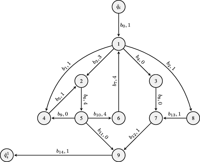

  

  A directed graph illustrating a graph $G_{\mathfrak {B}_{i}}$, where b_k, $0\leqslant k\leqslant 14$, denote the corresponding edges, the number after each b_k denotes the valuation of $y_{b_{k}}$

  Now we come back to the poof of the property that Eq. 35g can be equivalently specified by Eq. 36. Equivalently, we need to prove that Eqs. 35d, 35e, 35f, and 35g are all satisfied if and only if Eqs. 35d, 35e, 35f, and 36 are all satisfied. The “only if” part trivially holds. To prove the “if” part, we need to, for every i ∈ [[1, m]], for every edge $a_{i}\in A_{\mathfrak {B}_{i}}$ such that $y_{a_{i}}>0$ and $head(a_{i})\ne {\hat q_{i}^{1}}$, find a realizable path $\hat \pi _{i}$ from head(a_i) to ${\hat q_{i}^{1}}$. We claim that for a graph $G_{\mathfrak {B}_{i}}$ satisfying Eqs. 35d, 35e, 35f, and 36 (after $\bigwedge _{i\in \llbracket 1,m \rrbracket }$ was deleted), i ∈ [[1, m]], in every realizable cycle, if we subtract y_a for each edge a in the cycle by 1, then the rest of $G_{\mathfrak {B}_{i}}$ (denoted by $G_{\mathfrak {B}_{i}}^{\prime }$) still satisfies Eqs. 35d, 35e, 35f, and 36. One directly sees that if $G_{\mathfrak {B}_{i}}$ satisfies Eqs. 35d, 35e, 35f, then after doing such a subtraction, $G_{\mathfrak {B}_{i}}^{\prime }$ still satisfies Eqs. 35d, 35e, 35f. As one can see, for every realizable cycle in $G_{\mathfrak {B}_{i}}$, for every edge $a_{i}\in A_{\mathfrak {B}_{i}}$, either the cycle is contained in subgraph $G_{\mathfrak {B}_{i}}^{a_{i}}$ or it does not intersect with $G_{\mathfrak {B}_{i}}^{a_{i}}$.

  Fix a graph $G_{\mathfrak {B}_{i}}$, where i ∈ [[1, m]], that satisfies Eqs. 35d, 35e, 35f, and 36 (after $\bigwedge _{i\in \llbracket 1,m \rrbracket }$ was deleted). Fix a realizable simple cycle C and an edge $a_{i}\in A_{\mathfrak {B}_{i}}^{a_{i}}$ such that $y_{a_{i}}>0$ and $head(a_{i})\ne {\hat q_{i}^{1}}$. Without loss of generality, assume C is contained in $G_{\mathfrak {B}_{i}}^{a_{i}}$. Note that tail(a_i) is the source of subgraph $G_{\mathfrak {B}_{i}}^{a_{i}}$, so it satisfies

  $$ \begin{array}{@{}rcl@{}} \underset{\underset{head(a)=tail(a_{i})}{a\in A_{\mathfrak{B}_{i}}^{a_{i}}}}{\sum} y_{a}+1 = \underset{\underset{tail(a)=tail(a_{i})}{a\in A_{\mathfrak{B}_{i}}^{a_{i}}}}{\sum} y_{a}. \end{array} $$

  (37)

  • If a_i does not intersect with C, then after doing the subtraction (on C), a_i trivially satisfies Eq. 36.

  • If a_i intersects with C at head(a_i) but a_i is not contained in C, then after doing the subtraction, a_i still satisfies Eq. 36, because head(a_i) satisfies Eq. 35d.

  • If a_i is contained in C and a_i is a self-loop, then C coincides with a_i. After doing the subtraction we may have $y_{a_{i}}>0$ or $y_{a_{i}}=0$. In the former case, a_i naturally satisfies Eq. 36, in the latter case, a_i satisfies Eq. 36 vacuously, and on the other hand, because head(a_i) is the source (satisfying Eq. 37), there is $a\in A_{\mathfrak {B}_{i}}^{a_{i}}$ such that tail(a) = head(a_i) and y_a > 0.

  • If a_i is contained in C and a_i is not a self-loop, after doing the subtraction, if $y_{a_{i}}>0$ then a_i still satisfies Eq. 36 because head(a_i) satisfies Eq. 35d, if $y_{a_{i}}=0$, then a_i satisfies Eq. 36 vacuously, and there is $a\in A_{\mathfrak {B}_{i}}^{a_{i}}$ such that tail(a) = tail(a_i) and y_a > 0, because tail(a_i) is the source (satisfying Eq. 37).

  We have proved the above claim. We next repetitively trim $G_{\mathfrak {B}_{i}}^{a_{i}}$ by doing the above subtractions on realizable, simple cycles until we finally obtain a subgraph $trim(G_{\mathfrak {B}_{i}}^{a_{i}})$ in which there is no realized cycle. By the claim, we still have $trim(G_{\mathfrak {B}_{i}}^{a_{i}})$ satisfies Eqs. 35d, 35e, 35f, and 36. In addition, we have either (1) there is an edge b₁ in $trim(G_{\mathfrak {B}_{i}}^{a_{i}})$ such that tail(b₁) = head(a_i) and $y_{b_{1}}>0$, or, (2) there is an edge b₂ in $trim(G_{\mathfrak {B}_{i}}^{a_{i}})$ such that tail(b₂) = tail(a_i), $y_{b_{2}}>0$, and in the original graph $G_{\mathfrak {B}_{i}}^{a_{i}}$ there is a realizable path from head(a_i) to tail(a_i) (hence there is a realizable path from head(a_i) to head(b₂)). Since in $trim(G_{\mathfrak {B}_{i}}^{a_{i}})$ there is no realizable cycle and $trim(G_{\mathfrak {B}_{i}}^{a_{i}})$ satisfies Eq. 36, if we start from head(b₁) or head(b₂) and traverse realizable edges one by one, finally we will reach ${\hat q_{i}^{1}}$, thus we find a realizable path from head(a_i) to ${\hat q_{i}^{1}}$ in $G_{\mathfrak {B}_{i}}^{a_{i}}$. The proof of the “if” part has been finished.

  Example 11

  Reconsider the subgraph $G_{\mathfrak {B}_{i}}^{b_{0}}$ of graph $G_{\mathfrak {B}_{i}}$ shown in Fig. 8. After doing the above subtractions on its realizable cycles, we finally obtain $trim(G_{\mathfrak {B}_{i}}^{b_{0}})$ in Fig. 9.

  Fig. 9

  

  $trim(G_{\mathfrak {B}_{i}}^{b_{0}})$

  We find two realizable paths from 1 (i.e., head(b₀)) to ${\hat q_{i}^{1}}$. They are

  $$ \begin{array}{@{}rcl@{}} &&b_{1}b_{5}b_{6}b_{10}b_{7}b_{2}b_{13}b_{12}b_{14},\\ &&b_{2}b_{13}b_{12}b_{14}. \end{array} $$

  It is easy to see that $trim(G_{\mathfrak {B}_{i}}^{b_{0}})$ satisfies Eqs. 35d, 35e, 35f, and 36 (after $\bigwedge _{i\in \llbracket 1,m \rrbracket }$ was deleted).

  Now consider an arbitrary $j\in \llbracket 1,|\mathfrak {E}| \rrbracket$ and an arbitrary edge $a_{j}\in A_{\mathfrak {E}_{j}}$ such that $y_{a_{j}}>0$ and $head(a_{j})\ne {q_{j}^{1}}$. Compute a subgraph $G_{\mathfrak {E}_{j}}^{a_{j}}$ of graph $G_{\mathfrak {E}_{j}}$ that consists of a_j and all paths from head(a_j) to ${q_{j}^{1}}$ in time polynomial in the size of $G_{\mathfrak {E}_{j}}$. Analogously, we have Eqs. 35i, 35j, 35k, and 3.7.2 (after $\bigwedge _{j\in \llbracket 1,|\mathfrak {E}| \rrbracket }$ was deleted) are all satisfied if and only if Eqs. 35i, 35j, 35k, and

  $$ \begin{array}{@{}rcl@{}} \bigwedge\limits_{a_{j}\in A_{\mathfrak{E}_{j}}} \left( \begin{array}{c} y_{a_{j}} > 0 \wedge \\ head(a_{j})\ne {q_{j}^{1}} \end{array} \implies \underset{\underset{tail(a)=head(a_{j}) }{a\in A_{\mathfrak{E}_{j}}^{a_{j}}}}{\sum} y_{a}>0 \right) \end{array} $$

  (38)

  are all satisfied.

• (vii) Now we have obtained a Presburger formula Eq. 35 (after Eqs. 35g and 3.7.2 were replaced by Eqs. 36 and 38, respectively) in the form of Eq. 1. Next we show the formula has length polynomial in the size of $\mathcal {A}^{\mathbb {Z}}$. By Eqs. 35b and 35c, the formula has at most 2 quantifier alternations. It has 2 quantifier alternations if and only if ${\sum }_{i=1}^{m}|A_{\mathfrak {B}_{i}}|>0$ and ${\sum }_{j=1}^{|\mathfrak {E}|}|A_{\mathfrak {E}_{j}}|>0$. In Eqs. 35d, 35e, and 35f, the number of equations is bounded from above by ${\sum }_{i=1}^{m}|V_{\mathfrak {B}_{i}}| \leqslant |\hat x_{2}||Q|\leqslant |Q|^{2}$ (see (v)); in Eqs. 35i, 35j, and 35k, the number of equations has an upper bound ${\sum }_{i=1}^{|\mathfrak {E}|}|V_{\mathfrak {E}_{j}}| \leqslant |\mathfrak {E}| |Q| \leqslant |x_{1}||{\varDelta }_{\sigma }|(|x_{2}|-|\hat x_{2}|) |Q| \leqslant |Q|^{3}|{\varDelta }|$ (also see (v)); in Eq. 35h, the number of equations is bounded from above by $m-1\leqslant |Q|$; in Eq. 35l, the number of inequalities is bounded from above by $|\mathfrak {E}|\leqslant |x_{1}||{\varDelta }_{\sigma }|(|x_{2}|-|\hat x_{2}|) \leqslant |Q|^{2}|{\varDelta }|$; in Eq. 36, the number of inequalities is no greater than $2{\sum }_{i=1}^{m}|A_{\mathfrak {B}_{i}}| \leqslant 2m|{\varDelta }|\leqslant 2|Q||{\varDelta }|$; in Eq. 38, the number of inequalities is no greater than $2{\sum }_{j=1}^{|\mathfrak {E}|}|A_{\mathfrak {E}_{j}}|\leqslant 2|\mathfrak {E}||{\varDelta }|\leqslant 2|x_{1}||{\varDelta }_{\sigma }|(|x_{2}|-|\hat x_{2}|) |{\varDelta }| \leqslant 2|Q|^{2}|{\varDelta }|^{2}$. All these equations and inequalities have length polynomial in the size of $\mathcal {A}^{\mathbb {Z}}$. Hence Eq. 35 has length polynomial in the size of $\mathcal {A}^{\mathbb {Z}}$.

  • When Eq. 35 has 2 quantifier alternations, by Lemma 3, in the worst case we need to check all ${\sum }_{i=1}^{m}|A_{\mathfrak {B}_{i}}|+{\sum }_{j=1}^{|\mathfrak {E}|}|A_{\mathfrak {E}_{j}}|$ variables between 0 and $w=2^{cr^{(s+3)^{3}}}$ to make sure whether Eq. 35 is satisfied, where c is a constant, r is the length of Eq. 35, $s={\sum }_{i=1}^{m}|A_{\mathfrak {B}_{i}}|+{\sum }_{j=1}^{|\mathfrak {E}|}|A_{\mathfrak {E}_{j}}|$ is the number of quantifiers. The logarithm of w is exponential in the size of $\mathcal {A}^{\mathbb {Z}}$, and each check can be done in EXPTIME, hence the satisfiability of Eq. 35 can be checked in 2-EXPTIME in the size of $\mathcal {A}^{\mathbb {Z}}$.

  • When Eq. 35 has 1 quantifier alternation (in this case exactly one of ${\sum }_{i=1}^{m}|A_{\mathfrak {B}_{i}}|$ and ${\sum }_{j=1}^{|\mathfrak {E}|}|A_{\mathfrak {E}_{j}}|$ is equal to 0), one has $w=2^{cr^{(s+3)^{2}}}$. Hence the satisfiability of Eq. 35 can be checked also in 2-EXPTIME.

  • When Eq. 35 has 0 quantifier alternation, i.e., all graphs $G_{\mathfrak {B}_{i}}$, i ∈ [[1, m]], $G_{\mathfrak {E}_{j}}$, $j\in \llbracket 1,|\mathfrak {E}|\rrbracket$, are singletons, the satisfiability of Eq. 35 can be checked in polynomial time.

Remark 3

In (vi), the specifications of Eqs. 35g and 3.7.2 to 36 and 38 are crucial steps. If we did not do this but directly specify Eqs. 35g and 3.7.2 as they are, then Eq. 35 would have length exponential in the size of $\mathcal {A}^{\mathbb {Z}}$, and then the satisfiability of Eq. 35 would be checked in 3-EXPTIME in the size of $\mathcal {A}^{\mathbb {Z}}$ by using Lemma 3.

Taking graph $G_{\mathfrak {B}_{i}}^{a_{i}}$ for some i ∈ [[1, m]] for example, in order to directly specify Eq. 35g, we need to enumerate all α distinct (at most exponentially many) simple paths from head(a_i) to ${\hat q_{i}^{1}}$ as

$$ \begin{array}{@{}rcl@{}} &&a_{i}^{1,1}{\dots} a_{i}^{1,1_{\alpha}},\\ && {\vdots} \\ &&a_{i}^{\alpha,1}{\dots} a_{i}^{\alpha,\alpha_{\alpha}}, \end{array} $$

where $tail(a_{i}^{l,1})=head(a_{i})$, $head(a_{i}^{l,l_{\alpha }})= {\hat q_{i}^{1}}$, $head(a_{i}^{l,k_{l}})=tail(a_{i}^{l,k_{l}+1})$, $1\leqslant l\leqslant \alpha$, $1\leqslant l_{\alpha }\leqslant |V_{\mathfrak {B}_{i}}^{a_{i}}|-1$, $1\leqslant k_{l}\leqslant l_{\alpha }-1$. Equation 35g is directly specified as

$$\bigvee_{l=1}^{\alpha}\left( \bigwedge\limits_{k_{l}=1}^{l_{\alpha}} \left( y_{a_{i}^{l,k_{l}}}>0\right)\right),$$

which has length exponential in the size of $\mathcal {A}^{\mathbb {Z}}$.

Remark 4

Using the above procedure of computing observer $\mathcal {A}^{\mathbb {Q}^{k}}_{obs}$ as in Items (i) through (vii), one can do state estimation based on a given weighted label sequence $\gamma =(\sigma _{1},t_{1})\dots (\sigma _{n},t_{n})$, where σ_i ∈Σ, $t_{i}\in \mathbb {Q}^{k}$, i ∈ [[1, n]]: first, compute all states q₁ that are reachable from some state of Q₀ through some unobservable path followed by some observable transition with an event e₁ in $E_{\sigma _{1}}$, where the entire path has weight t, in nondeterministic polynomial time by Lemma 1, denote the set of all such q₁ by x₁, and call x₁ the (σ₁, t₁)-successor of Q₀; second, compute the (σ₂, t₂ − t₁)-successor x₂ of x₁; …; finally compute the (σ_n, t_n − t_n− 1)-successor x_n of x_n− 1, then one has ${\mathscr{M}}(\mathcal {A}^{\mathbb {Q}^{k}},\epsilon |x_{n})={\mathscr{M}}(\mathcal {A}^{\mathbb {Q}^{k}},\gamma )$.

Now we analyze the complexity of computing $\mathcal {A}_{obs}^{\mathbb {Z}}$. For every x₁ ⊂ Q (see (i)), we compute the corresponding x₂ in polynomial time. For every $\bar x_{2}\subset x_{2}$ (see (ii)), we check whether $\bar x_{2}$ is a successor of x₁ and compute the corresponding transitions starting from x₁ in $\mathcal {A}_{obs}^{\mathbb {Z}}$ as follows: we compute automaton (30) for at most $(|x_{1}||{\varDelta }_{\sigma }|)^{|\bar x_{2}|}$ times (see (ii) and (iii)). Then in each automaton (32) (trivially obtained from Eq. 30) (see (iv)), we check the existence of path $\bar \pi$ (see Eq. B) and compute transitions of $\mathcal {A}_{obs}^{\mathbb {Z}}$ starting at x₁ in NP in the size of Eq. 32 by Lemma 1, where the size of Eq. 32 is exponential in the size of $\mathcal {A}^{\mathbb {Z}}$. Totally we check the existence of $\bar \pi$ in Eq. 32 for at most exponentially many times. Hence this part can be finished in NEXPTIME in the size of $\mathcal {A}^{\mathbb {Z}}$.

Consider the above x₁ and x₂, for every successor $\bar x_{2}\subset x_{2}$ of x₁ computed as above, for every subset $\hat x_{2}\subsetneq \bar x_{2}$, we check whether there is a transition from x₁ to ${\mathscr{M}}(\mathcal {A}^{\mathbb {Z}},\epsilon |\hat x_{2})$ as in (v), (vi), (vii). When $x_{1},x_{2},\hat x_{2}$ are given, $\mathfrak {E}$ (see Eq. 34) is also given, we need to check the satisfiability of Presburger formula Eq. 35 by Lemma 3 for at most $(|x_{1}||{\varDelta }_{\sigma }|)^{|\hat x_{2}|}$ times. Totally we do the check for at most exponentially many times. Hence this part can be finished in 2-EXPTIME in the size of $\mathcal {A}^{\mathbb {Z}}$.

Theorem 8

An observer ${\mathcal {A}}_{obs}^{\mathbb {Q}^{k}}$ (21) of a labeled weighted automaton $\mathcal {A}^{\mathbb {Q}^{k}}$ can be computed in 2-EXPTIME in the size of $\mathcal {A}^{\mathbb {Q}^{k}}$.

Particularly, for deadlock-free and divergence-free automaton $\mathcal {A}^{\mathbb {Q}^{k}}$, in which there exists no unobservable cycle, from the above procedure of computing ${\mathcal {A}}{^{\mathbb {Q}^{k}}_{obs}}$, one directly sees that the EPL problem and Presburger arithmetic are not needed, but one only needs to enumerate all (exponentially many) unobservable paths. Hence the next direct corollary follows.

Corollary 2

The observer ${\mathcal {A}}_{obs}^{\mathbb {Q}^{k}}$ (21) of a divergence-free $\mathcal {A}^{\mathbb {Q}^{k}}$ can be computed in EXPTIME in the size of $\mathcal {A}^{\mathbb {Q}^{k}}$.

In Theorem 4, conditions (i) and (ii) can be verified in time linear in the size of $\mathcal {A}^{\mathbb {Q}^{k}}$ by computing its strongly connected components, and condition (iii) can be verified in time linear in the size of any observer ${\mathcal {A}}{^{\mathbb {Q}^{k}}_{obs}}$. Then the following result holds.

Theorem 9

The weak detectability of a labeled weighted automaton $\mathcal {A}^{\mathbb {Q}^{k}}$ can be verified in 2-EXPTIME in the size of $\mathcal {A}^{\mathbb {Q}^{k}}$.

Similarly, by Theorems 5 and 8, the following result holds.

Theorem 10

The weak periodic detectability of a labeled weighted automaton $\mathcal {A}^{\mathbb {Q}^{k}}$ can be verified in 2-EXPTIME in the size of $\mathcal {A}^{\mathbb {Q}^{k}}$.

By Theorems 4 and 5, and Corollary 2, the following result holds.

Corollary 3

The weak detectability and weak periodic detectability of a labeled deadlock-free, divergence-free weighted automaton $\mathcal {A}^{\mathbb {Q}^{k}}$ can be verified in EXPTIME in the size of $\mathcal {A}^{\mathbb {Q}^{k}}$. The upper bounds also apply to deadlock-free and divergence-free unambiguous weighted automata over semiring $\underline {\mathbb {Q}}$.

When all transitions of $\mathcal {A}^{\mathbb {Q}^{k}}$ are observable, we have the following direct corollary.

Corollary 4

Consider a labeled weighted automaton $\mathcal {A}^{\mathbb {Q}^{k}}$ all of whose transitions are observable. Its observer ${\mathcal {A}}{^{\mathbb {Q}^{k}}_{obs}}$ can be computed in EXPTIME, and its weak detectability and weak periodic detectability can be verified also in EXPTIME.

3.7.3 Computation of detector $\mathcal {A}_{det}^{\mathbb {Q}^{k}}$ and verification of strong periodic detectability

One sees detector ${\mathcal {A}}_{det}^{\mathbb {Q}^{k}}$ (23) is a simplified version of observer ${\mathcal {A}}_{obs}^{\mathbb {Q}^{k}}$ (21), hence ${\mathcal {A}}_{det}^{\mathbb {Q}^{k}}$ can be computed similarly by starting from the initial state $x_{0}={\mathscr{M}}(\mathcal {A}^{\mathbb {Q}^{k}},\epsilon )$, and find all reachable states and transitions step by step, where the states (except for x₀) are of cardinality $\leqslant 2$. Similarly to (i) in Section 3.7.2, choose a state x₁ ∈ X of $\mathcal {A}_{det}^{\mathbb {Q}^{k}}$ that we have just computed (here $1\leqslant |x_{1}|\leqslant 2$ if x₁≠x₀), choose σ ∈Σ, for each q ∈ x₁, compute subautomaton $\mathcal {A}_{q}^{\mathbb {Q}^{k}}$ that consists of all paths of the form

$$ q\xrightarrow[]{s}q^{1}\xrightarrow[]{e}q^{2} $$

(39)

of $\mathcal {A}^{\mathbb {Q}^{k}}$ such that s ∈ (E_uo)^∗, e ∈ E_σ. Denote the set of all such q² by x₂. Note that one may have |x₂| > 2.

• 1. If $|{\mathscr{M}}(\mathcal {A}^{\mathbb {Q}^{k}},\epsilon |x_{2})|=1$ (i.e., ${\mathscr{M}}(\mathcal {A}^{\mathbb {Q}^{k}},\epsilon |x_{2})=x_{2}$ and x₂ is a singleton), then we find a transition $x_{1}\xrightarrow []{(\sigma ,t)} x_{2}$ of $\mathcal {A}^{\mathbb {Q}^{k}}_{det}$, where t can be the weight of any path from any q in x₁ to the unique q² in x₂ as in Eq. 39.

• 2. If $|{\mathscr{M}}(\mathcal {A}^{\mathbb {Q}^{k}},\epsilon |x_{2})|>1$, for every $\bar x_{2}\subset x_{2}$ with $|\bar x_{2}|=2$, we check whether there exists two paths

  $$ \begin{array}{@{}rcl@{}} q_{i} \xrightarrow[]{s_{i}}{q^{1}_{i}}\xrightarrow[]{e_{i}}{q^{2}_{i}},\quad i=1,2, \end{array} $$

  as in Eq. 39, such that q_i ∈ x₁, $\{{q_{1}^{2}},{q_{2}^{2}}\}=\bar x_{2}$, and the two paths have the same weight $t\in \mathbb {Q}^{k}$. If the answer is YES, then we find transitions $x_{1}\xrightarrow []{(\sigma ,t)}\bar x_{2}^{\prime }$ for any $\bar x_{2}^{\prime }\subset {\mathscr{M}}(\mathcal {A}^{\mathbb {Q}^{k}},\epsilon |\bar x_{2})$ with $|\bar x_{2}^{\prime }|=2$. In each of these checks, we need to compute the synchronous product (see Eq. 30) of two subautomata of $\mathcal {A}^{\mathbb {Q}^{k}}$ (in polynomial time), and solve a 1-dimensional EPL problem in the product (by Lemma 1, in NP).

• 3. If $|{\mathscr{M}}(\mathcal {A}^{\mathbb {Q}^{k}},\epsilon |x_{2})|>1$, for every $\bar x_{2}\subset x_{2}$ with $|\bar x_{2}|=1$ and $|{\mathscr{M}}(\mathcal {A}^{\mathbb {Q}^{k}},\epsilon |\bar x_{2})|>1$, we find transitions $x_{1}\xrightarrow []{(\sigma ,t)} \bar x_{2}^{\prime }$ for any $\bar x_{2}^{\prime }\subset {\mathscr{M}}(\mathcal {A}^{\mathbb {Q}^{k}},\epsilon |\bar x_{2})$ with $|\bar x_{2}^{\prime }|=2$, where t can be the weight of any path from any q in x₁ to the unique q² in $\bar x_{2}$ as in Eq. 39.

• 4. If $|{\mathscr{M}}(\mathcal {A}^{\mathbb {Q}^{k}},\epsilon |x_{2})|>1$, for every $\bar x_{2}\subset x_{2}$ with $|{\mathscr{M}}(\mathcal {A}^{\mathbb {Q}^{k}},\epsilon |\bar x_{2})|=1$, we check whether

  there exists a path

  $$ \begin{array}{@{}rcl@{}} \hat q \xrightarrow[]{\hat s}\hat q^{1}\xrightarrow[]{\hat e}\hat q^{2} \end{array} $$

  as in Eq. 39, such that $\hat q\in x_{1}$, $\{\hat q^{2}\}=\bar x_{2}$, the weight of the path is denoted by $t\in \mathbb {Q}^{k}$; and for any $\bar q\in x_{1}$, for any $q^{2}\in x_{2}\setminus \bar x_{2}$, there is no path

  $$ \begin{array}{@{}rcl@{}} q \xrightarrow[]{s}q^{1}\xrightarrow[]{e}q^{2} \end{array} $$

  as in Eq. 39 with weight t. (G)

  If the answer is YES, then we find a transition $x_{1}\xrightarrow []{(\sigma ,t)}\bar x_{2}$ of $\mathcal {A}^{\mathbb {Q}^{k}}_{det}$. We need to transform the satisfiability of Eq. G to satisfiability of some Presburger formula as in (v), (vi), (vii). By Lemma 3, such checks can be done in 2-EXPTIME.

Theorem 11

Consider a labeled weighted automaton $\mathcal {A}^{\mathbb {Q}^{k}}$. An detector $\mathcal {A}^{\mathbb {Q}^{k}}_{det}$ can be computed in 2-EXPTIME (in the size of $\mathcal {A}^{\mathbb {Q}^{k}}$); particularly if for each state q of $\mathcal {A}^{\mathbb {Q}^{k}}$, $|{\mathscr{M}}(\mathcal {A}^{\mathbb {Q}^{k}},\epsilon |\{q\})|>1$ (in this case, one need not check the satisfiability of Eq. G), then $\mathcal {A}^{\mathbb {Q}^{k}}_{det}$ can be computed in NP.

By Theorem 3, the following result holds.

Theorem 12

Consider a labeled weighted automaton $\mathcal {A}^{\mathbb {Q}^{k}}$. Its strong periodic detectability can be verified in 2-EXPTIME. Particularly, if for each state q of $\mathcal {A}^{\mathbb {Q}^{k}}$, $|{\mathscr{M}}(\mathcal {A}^{\mathbb {Q}^{k}},\epsilon |\{q\})|>1$, then its strong periodic detectability can be checked in NP.

By Theorem 2 and Corollary 2, the following two results hold.

Theorem 13

The problem of verifying strong periodic detectability of a deadlock-free and divergence-free $\mathcal {A}^{\mathbb {Q}^{k}}$ belongs to EXPTIME.

Corollary 5

The detector ${\mathcal {A}}_{det}^{\mathbb {Q}^{k}}$ (23) of a divergence-free $\mathcal {A}^{\mathbb {Q}^{k}}$ can be computed in EXPTIME in the size of $\mathcal {A}^{\mathbb {Q}^{k}}$.

Similarly to the case of $CC_{A}(\mathcal {A}^{\mathbb {Q}^{k}})$, we have the following direct corollary.

Corollary 6

Consider a labeled weighted automaton $\mathcal {A}^{\mathbb {Q}^{k}}$ all of whose transitions are observable. Its detector ${\mathcal {A}}{\mathbb {Q}^{k}}_{det}$ can be computed in polynomial time, and its strong periodic detectability can be verified also in polynomial time.

For a labeled finite-state automaton $\mathcal {A}$, one directly sees from the above procedure of computing ${\mathcal {A}}{\mathbb {Q}^{k}}_{det}$ that detector $\mathcal {A}_{det}$ can be computed in polynomial time, because all unobservable transitions of $\mathcal {A}$ have weight 0 as shown in Remark 1. Then the following corollary holds.

Corollary 7

The strong periodic detectability of a labeled finite-state automaton $\mathcal {A}$ can be verified in polynomial time.

3.7.4 The complexity lower bounds on verifying strong (periodic) detectability of labeled weighted automaton

$\mathcal {A}^{\mathbb {N}}$ and $\mathcal {A}^{\underline {\mathbb {N}}}$

In this subsection, we prove coNP lower bounds on verifying strong detectability and strong periodic detectability of labeled deterministic weighted automata over monoid $(\mathbb {N},+,0)$. These complexity lower bounds also apply to strong detectability and strong periodic detectability of labeled deterministic weighted automata over semiring $\underline {\mathbb {N}}$, because deterministic automata are unambiguous, and the definitions of detectability for unambiguous $\mathcal {A}^{\underline {\mathbb {Q}}}$ in Lai et al. (2021a) coincide with those for unambiguous $\mathcal {A}^{\mathbb {Q}}$ in the current paper (except for minor and neglectable differences, see Remark 8 of Appendix). As a result, deterministic $\mathcal {A}^{\mathbb {N}}$ and $\mathcal {A}^{\underline {\mathbb {N}}}$ are fundamentally more complicated than labeled finite-state automata, because it is known that strong (periodic) detectability of labeled finite-state automata can be verified in polynomial time (Shu and Lin 2011; Zhang and Giua 2019).

Theorem 14

The problems of verifying strong detectability and strong periodic detectability of labeled deterministic, deadlock-free, and divergence-free weighted automaton $\mathcal {A}^{\mathbb {N}}$ and $\mathcal {A}^{\underline {\mathbb {N}}}$ are both coNP-hard.

Proof

We reduce the NP-complete subset sum problem (Problem 2) to negation of strong detectability and strong periodic detectability of labeled deterministic weighted automata over $\mathbb {N}$ (hence also over $\underline {\mathbb {N}}$).

Given positive integers $n_{1},\dots ,n_{m}$, and N, next we construct in polynomial time a labeled deterministic weighted automaton $\mathcal {A}_{2}^{\mathbb {N}}$ as illustrated in Fig. 10. Apparently, $\mathcal {A}_{2}^{\mathbb {N}}$ is deadlock-free and divergence-free. q₀ is the unique initial state and has initial time delay 0. Events u₁, u₂ are unobservable. Event e is observable and ℓ(e) = e. For all i ∈ [[0, m − 1]], there exist two unobservable transitions $q_{i}\xrightarrow []{u_{1}/n_{i+1}}q_{i+1}$ and $q_{i}\xrightarrow []{u_{2}/0}q_{i+1}$. The observable transitions are $q_{m}\xrightarrow []{e/1}q_{m+1}^{1}$, $q_{0}\xrightarrow []{e/N+1}q_{m+1}^{2}$, and two self-loops $q_{m+1}^{1}\xrightarrow []{e/1}q_{m+1}^{1}$ and $q_{m+1}^{2}\xrightarrow []{e/1}q_{m+1}^{2}$.

Fig. 10

Sketch of the reduction in the proof of Theorem 14

Suppose there exists I ⊂[[1, m]] such that $N={\sum }_{i\in I}n_{i}$. Then there is an unobservable path $\pi \in q_{0}\rightsquigarrow q_{m}$ whose weight is equal to N. Then we have

$$ \begin{array}{@{}rcl@{}} \ell(\tau(\pi\xrightarrow[]{e}q_{m+1}^{1})) &=& (e,N+1), \end{array} $$

(40)

$$ \begin{array}{@{}rcl@{}} \mathcal{M}(\mathcal{A}_{2}^{\mathbb{N}},(e,N+1)\dots(e,N+k)) &=& \{q_{m+1}^{1},q_{m+1}^{2}\} \end{array} $$

(41)

for all $k\in \mathbb {Z}_{+}$.

Choose

$$w=\tau(\pi\xrightarrow[]{e}q_{m+1}^{1}(\xrightarrow[]{e}q_{m+1}^{1})^{\omega})\in L^{\omega}(\mathcal{A}_{2}^{\mathbb{N}}).$$

Then

$$\ell(w)=(e,N+1)(e,N+2)\dots.$$

Choose prefix $\gamma _{k}=(e,N+1)\dots (e,N+k)\sqsubset \ell (w)$. Then we have $|\gamma _{k}|\geqslant k$ and $|{\mathscr{M}}(\mathcal {A}_{2}^{\mathbb {N}}, \gamma _{k})|>1$ by Eq. 41. Hence $\mathcal {A}_{2}^{\mathbb {N}}$ is not strongly detectable.

For all $k\in \mathbb {N}$, choose the above w, choose $w^{\prime }=\tau (\pi \xrightarrow []{e}q_{m+1}^{1})\sqsubset w$, for all $w^{\prime \prime }$ such that $w^{\prime }w^{\prime \prime }\sqsubset w$ and $|\ell (w^{\prime \prime })|<k$, we have $|{\mathscr{M}}(\mathcal {A}_{2}^{\mathbb {N}},\ell (w^{\prime }w^{\prime \prime }))|>1$ by Eq. 41. Hence $\mathcal {A}_{2}^{\mathbb {N}}$ is not strongly periodically detectable.

Suppose for all I ⊂[[1, m]], $N\ne {\sum }_{i\in I}n_{i}$. Then for all $\pi ^{\prime }\in q_{0}\rightsquigarrow q_{m}$, one has

$$ \begin{array}{@{}rcl@{}} \ell(\tau(\pi^{\prime}\xrightarrow[]{e}q_{m+1}^{1})) &=& (e,N^{\prime}+1)\text{ for some }N^{\prime}\ne N,\\ \mathcal{M}(\mathcal{A}_{2}^{\mathbb{N}},\ell(\tau(\pi^{\prime}\xrightarrow[]{e}q_{m+1}^{1}))) &=& \{q_{m+1}^{1}\},\\ \mathcal{M}(\mathcal{A}_{2}^{\mathbb{N}},(e,N^{\prime}+1)\dots(e,N^{\prime}+k)) &=& \{q_{m+1}^{1}\},\\ \mathcal{M}(\mathcal{A}_{2}^{\mathbb{N}},(e,N+1)\dots(e,N+k)) &=& \{q_{m+1}^{2}\} \end{array} $$

for all $k\in \mathbb {Z}_{+}$. Hence $\mathcal {A}_{2}^{\mathbb {N}}$ is strongly detectable and strongly periodically detectable. □

The next corollary directly follows from Theorems 7 and 14.

Corollary 8

The problems of verifying strong detectability of labeled unambiguous weighted automaton $\mathcal {A}^{\mathbb {Q}^{k}}$ and $\mathcal {A}^{\underline {\mathbb {Q}}}$ are both coNP-complete.

3.8 Illustrative examples

In this subsection, we illustrate how to use Theorems 1, 3, 4, and 5 to verify strong (periodic) detectability and weak (periodic) detectability of labeled weighted automata over monoid $(\mathbb {N},+,0)$ and labeled unambiguous weighted automata over semiring $\underline {\mathbb {N}}$.

Example 12

Reconsider labeled unambiguous weighted automaton $\mathcal {A}_{0}^{\mathbb {N}}$ (the same as $\mathcal {A}_{0}^{\underline {\mathbb {N}}}$) in Fig. 3. Its detectability cannot be verified by using the method developed in Lai et al. (2021a) (see Remark 9 of Appendix). Next we show how to verify its detectability by using the methods proposed in the current paper.

Its self-composition $CC_{A}(\mathcal {A}_{0}^{\mathbb {N}})$ is shown in Fig. 11. The self-loops on (q₃, q₄) and on (q₄, q₃) are easy to find. We use the method developed in Section 3.7.1 to check whether there exists a transition ((q₀, q₀),(a, a),(q₃, q₄)): (1) Guess transitions $q_{1}\xrightarrow []{a/1}q_{3}$ and $q_{2}\xrightarrow [] {a/1}q_{4}$ of $\mathcal {A}_{0}^{\mathbb {N}}$. (2) Compute subautomaton $\mathcal {A}_{q_{0}}^{\mathbb {N}}$ as in Fig. 12 and asynchronous product $\mathcal {A}_{q_{0}}^{\mathbb {N}}\otimes \mathcal {A}_{q_{0}}^{\mathbb {N}}$ as in Fig. 13 and check in weighted directed graph $\mathcal {A}_{q_{0}}^{\mathbb {N}}\otimes \mathcal {A}_{q_{0}}^{\mathbb {N}}$, whether there exists a path from (q₀, q₀) to (q₁, q₂) with weight 0. By using the solution to the 1-dimensional EPL problem given by Nykänen and Ukkonen (2002), we can find several such paths, e.g., $(q_{0},q_{0})\left (\xrightarrow []{-1} (q_{0},q_{2}) \right )^{9}\xrightarrow []{10} (q_{1},q_{2})$.

Fig. 11

Self-composition $CC_{A}(\mathcal {A}_{0}^{\mathbb {N}})$ of the automaton $\mathcal {A}_{0}^{\mathbb {N}}$ in Fig. 3

Fig. 12

Subautomaton $\mathcal {A}_{q_{0}}^{\mathbb {N}}$ of the automaton $\mathcal {A}_{0}^{\mathbb {N}}$ in Fig. 3

Fig. 13

Asynchronous product $\mathcal {A}_{q_{0}}^{\mathbb {N}}\otimes \mathcal {A}_{q_{0}}^{\mathbb {N}}$ of subautomaton $\mathcal {A}_{q_{0}}^{\mathbb {N}}$ (in Fig. 12) of the automaton $\mathcal {A}_{0}^{\mathbb {N}}$ in Fig. 3

In $CC_{A}(\mathcal {A}_{0}^{\mathbb {N}})$, there exists a self-loop on the reachable state (q₃, q₄), then a transition sequence as in Eq. 24 exists. In addition, in $\mathcal {A}_{0}^{\mathbb {N}}$, there exists a self-loop on q₃, then (ii) of Theorem 1 holds. By Theorem 1, $\mathcal {A}_{0}^{\mathbb {N}}$ is not strongly detectable. By definition, we choose infinite path $q_{0}\xrightarrow []{u}q_{1}\left (\xrightarrow []{a}q_{3} \right )^{\omega }$, and choose path $\pi _{n}=q_{0}\xrightarrow []{u}q_{1}\left (\xrightarrow []{a}q_{3} \right )^{n}$, then we have $\ell (\tau (\pi _{n}))=(a,11)\dots (a,10+n)$, and ${\mathscr{M}}(\mathcal {A}_{0}^{\mathbb {N}},\ell (\tau (\pi _{n})))= \{q_{3},q_{4}\}$, hence we also have $\mathcal {A}_{0}^{\mathbb {N}}$ is not strongly detectable.

One observer ${\mathcal {A}}{_{0obs}^{\mathbb {N}}}$ (also detector ${\mathcal {A}}{_{0det}^{\mathbb {N}}}$) is shown in Fig. 14. We use the method developed in Section 3.7.2 to check whether $\{q_{0}\}\xrightarrow []{(a,11)}\{q_{3},q_{4}\}$ and $\{q_{0}\}\xrightarrow []{(a,2)}\{q_{4}\}$ are transitions of ${\mathcal {A}}{_{0obs}^{\mathbb {N}}}$. For the former, by the path $(q_{0},q_{0})\left (\xrightarrow []{-1} (q_{0},q_{2}) \right )^{9}\xrightarrow []{10} (q_{1},q_{2})$ with weight 0 in Fig. 13 and transitions $q_{1}\xrightarrow []{a/1}q_{3}$ and $q_{2}\xrightarrow []{a/1}q_{4}$, we know that {q₃, q₄} is a successor of {q₀} (see (iii) in Section 3.7.2), and then obtain the transition $\{q_{0}\}\xrightarrow []{(a,11)}{\mathscr{M}}(\mathcal {A}_{0}^{\mathbb {N}},\epsilon |\{q_{3},q_{4}\})$, where ${\mathscr{M}}(\mathcal {A}_{0}^{\mathbb {N}},\epsilon |\{q_{3},q_{4}\})=\{q_{3},q_{4}\}$; for the latter, one sees a transition sequence $q_{0}\xrightarrow []{u/1}q_{2}\xrightarrow []{a/1}q_{4}$ with weight 2, but the unique transition sequence from q₀ to q₃ is $q_{0}\xrightarrow []{u/10}q_{1}\xrightarrow []{a/1}q_{3}$ having weight 11 that is not equal to 2, so $\{q_{0}\}\xrightarrow []{(a,2)}\{q_{4}\}$ is also a transition. On the other hand, since there is a transition sequence $q_{0}\left (\xrightarrow []{u/1}q_{2}\right )^{10}\xrightarrow []{a/1}q_{4}$ having the same weight as $q_{0}\xrightarrow []{u/10}q_{1}\xrightarrow []{a/1}q_{3}$, there is no transition from {q₀} to ${\mathscr{M}}(\mathcal {A}_{0}^{\mathbb {N}}, \epsilon |\{q_{3}\})=\{q_{3}\}$. In observer ${\mathcal {A}}{_{0obs}^{\mathbb {N}}}$ (also detector ${\mathcal {A}}{_{0det}^{\mathbb {N}}}$), there is a self-loop on a reachable state {q₃, q₄} of cardinality 2, then (2) of Theorem 3 holds, hence $\mathcal {A}_{0}^{\mathbb {N}}$ is not strongly periodically detectable. Consider infinite path $\pi =q_{0}\left (\xrightarrow []{u}q_{2} \right )^{\omega }$, one has $\tau (\pi )=(u,1)(u,2)\dots$, and $\ell (\tau (\pi ))=\epsilon \in (\{a\}\times \mathbb {N})^{*}$, then (ii) of Theorem 4 holds, and $\mathcal {A}_{0}^{\mathbb {N}}$ is weakly detectable. Moreover, one has ${\mathscr{M}}(\mathcal {A}_{0}^{\mathbb {N}},\epsilon )=\{q_{0}\}$, then (ii) of Theorem 5 holds, and $\mathcal {A}_{0}^{\mathbb {N}}$ is weakly periodically detectable.

Fig. 14

One observer ${\mathcal {A}}{_{0obs}^{\mathbb {N}}}$ (also detector ${\mathcal {A}}{_{0det}^{\mathbb {N}}}$) of the automaton $\mathcal {A}_{0}^{\mathbb {N}}$ in Fig. 3

Example 13

Reconsider automaton $\mathcal {A}_{1}^{\mathbb {N}}$ shown in Fig. 4.

In its self-composition shown in Fig. 5, there exists a unique cycle, i.e., a self-loop on state (q₄, q₄); there exists no state of the form $(q,q^{\prime })$ satisfying $q\ne q^{\prime }$ reachable from the unique cycle. Then there exists no transition sequence shown in Eq. 24. By Theorem 1, $\mathcal {A}_{1}^{\mathbb {N}}$ is strongly detectable. By definition, $\mathcal {A}_{1}^{\mathbb {N}}$ is strongly detectable by choosing k = 2.

In one of its detectors obtained from Fig. 6 by changing $\mathbb {Z}_{+}$ to 1, there exists a reachable state {q₁, q₂} satisfying |{q₁, q₂}| > 1, and in $\mathcal {A}_{1}^{\mathbb {N}}$, there exists an unobservable self-loop on q₁. Then (1) in Theorem 3 is satisfied, so $\mathcal {A}_{1}^{\mathbb {N}}$ is not strongly periodically detectable. By definition, for all $k\in \mathbb {N}$, choose $w_{k}=\tau \left (q_{0}\xrightarrow []{a}q_{1}\left (\xrightarrow []{u}q_{1} \right )^{\omega }\right )=(a,1)(u,2) (u,3)\dots$, $w^{\prime }=(a,1)\sqsubset w_{k}$; for all $w^{\prime \prime }=(u,2)\dots (u,i)\sqsubset (u,2)(u,3)\dots$, one has $w^{\prime }w^{\prime \prime }\sqsubset w_{k}$, $\ell (w^{\prime \prime })=\epsilon$, and ${\mathscr{M}}(\mathcal {A}_{1}^{\mathbb {N}},\ell (w^{\prime }w^{\prime \prime }))={\mathscr{M}}(\mathcal {A}_{1}^{\mathbb {N}}, (a,1))=\{q_{1},q_{2}\}$, so $\mathcal {A}_{1}^{\mathbb {N}}$ is not strongly periodically detectable.

In one of its observers also obtained from Fig. 6 by changing $\mathbb {Z}_{+}$ to 1, one sees that (iii) in Theorem 4 is satisfied, so $\mathcal {A}_{1}^{\mathbb {N}}$ is weakly detectable. On the other hand, we have $(a,1)(u,2)(u,3)\dots \in L^{\omega }(\mathcal {A}_{1}^{\mathbb {N}})$ such that $\ell ((a,1)(u,2)(u,3)\dots )=(a,1)\in ({\varSigma }\times \mathbb {N})^{+}$, (ii) of Theorem 4 is also satisfied, one then also has $\mathcal {A}_{1}^{\mathbb {N}}$ is weakly detectable. Similarly, (iii) in Theorem 5 is satisfied, so $\mathcal {A}_{1}^{\mathbb {N}}$ is weakly periodically detectable.

Example 14

Reconsider automaton $\mathcal {A}^{\mathbb {N}}_{2}$ in the proof of Theorem 14 (in Fig. 10).

Assume that the subset sum problem has a solution, that is, there exists I ⊂[[1, m]] such that $N={\sum }_{i\in I}n_{i}$. We consider m > 1.

The self-composition of $\mathcal {A}^{\mathbb {N}}_{2}$ is shown in Fig. 15. The initial state (q₀, q₀) transitions to a self-loop on $(q_{m+1}^{1},q_{m+1}^{2})$ and then also to the state $(q_{m+1}^{1},q_{m+1}^{2})$ such that $q_{m+1}^{1}\ne q_{m+1}^{2}$. In $\mathcal {A}^{\mathbb {N}}_{2}$, there is a self-loop on $q_{m+1}^{1}$. Then by Theorem 1, $\mathcal {A}^{\mathbb {N}}_{2}$ is not strongly detectable.

Fig. 15

Self-composition of $\mathcal {A}^{\mathbb {N}}_{2}$ in Fig. 10 when the subset sum problem has a solution

The observers (also the detectors) of $\mathcal {A}^{\mathbb {N}}_{2}$ are shown in Fig. 16. The initial state x₀ transitions to a self-loop on $\{q_{m+1}^{1},q_{m+1}^{2}\}$, where $\{q_{m+1}^{1},q_{m+1}^{2}\}$ is of cardinality 2, then (ii) of Theorem 2 and (2) of Theorem 3 are satisfied. By Theorems 2 or 3, $\mathcal {A}^{\mathbb {N}}_{2}$ is not strongly periodically detectable. On the other hand, x₀ transitions to a self-loop on $\{q_{m+1}^{1}\}$, where $\{q_{m+1}^{1}\}$ is of cardinality 1, then (iii) of Theorem 4 is satisfied. By Theorem 4, $\mathcal {A}^{\mathbb {N}}_{2}$ is weakly detectable. In addition, (iii) of Theorem 5 is satisfied. By Theorem 5, $\mathcal {A}^{\mathbb {N}}_{2}$ is weakly periodically detectable.

Fig. 16

Observers (also detectors) of $\mathcal {A}^{\mathbb {N}}_{2}$ in Fig. 10 when the subset sum problem has a solution, where $x_{0}={\mathscr{M}}(\mathcal {A}^{\mathbb {N}}_{2},\epsilon )=\{q_{0},\dots ,q_{m}\}$, U can be the sum of elements of any subset of $\{n_{1},\dots ,n_{m}\}$ different from N

Assume that the subset sum problem has no solution, that is, for all I ⊂[[1, m]], $N\ne {\sum }_{i\in I}n_{i}$.

The self-composition of $\mathcal {A}^{\mathbb {N}}_{2}$ is shown in Fig. 17, in which there is no reachable state of the form $(q,q^{\prime })$ such that $q\ne q^{\prime }$. Then by Theorem 1, $\mathcal {A}^{\mathbb {N}}_{2}$ is strongly detectable.

Fig. 17

Self-composition of $\mathcal {A}^{\mathbb {N}}_{2}$ in Fig. 10 when the subset sum problem has no solution

The observers (also the detectors) of $\mathcal {A}^{\mathbb {N}}_{2}$ are shown in Fig. 18. The initial state x₀ satisfies that |x₀| > 1, but there is no unobservable cycle in $\mathcal {A}^{\mathbb {N}}_{2}$, that is, (1) of Theorem 3 is not satisfied. Apparently, (2) of Theorem 3 is not satisfied either. Hence $\mathcal {A}^{\mathbb {N}}_{2}$ is strongly periodically detectable. Here x₀ also transitions to a self-loop in which the state is of cardinality 1 (e.g., $\{q_{m+1}^{1}\}$), then by Theorems 4 and 5, $\mathcal {A}^{\mathbb {N}}_{2}$ is weakly detectable and weakly periodically detectable.

Fig. 18

Observers (also detectors) of $\mathcal {A}^{\mathbb {N}}_{2}$ in Fig. 10 when the subset sum problem has no solution, where $x_{0}={\mathscr{M}}(\mathcal {A}^{\mathbb {N}}_{2},\epsilon )=\{q_{0},\dots ,q_{m}\}$, U can be the sum of elements of any subset of $\{n_{1},\dots ,n_{m}\}$

4 Initial exploration of detectability in labeled timed automata

As mentioned in the last paragraph of Section 1.1, a labeled weighted automaton $\mathcal {A}^{\mathbb {Q}_{\geqslant 0}}$ is actually a one-clock labeled timed automaton in which the clock is reset along with every occurrence of every event and all clock constraints are singletons. In this section, we initially explore detectability in general labeled timed automata, and show some relations between a labeled weighted automaton $\mathcal {A}^{\mathfrak {M}}$ and a labeled timed automaton $\mathcal {A}^{\mathfrak {T}}$.

4.1 Notation

Let Σ be an alphabet, a timed word over Σ is a finite sequence $(a_{1},t_{1})\dots (a_{n},t_{n})$, where $n\in \mathbb {N}$, $a_{1},\dots ,a_{n}\in {\varSigma }$, $t_{1},\dots ,t_{n}\in \mathbb {R}_{\geqslant 0}$, $t_{1}\leqslant {\cdots } \leqslant t_{n}$. The set of timed words over Σ is denoted by TW^∗(Σ). An ω-timed word over Σ is an infinite sequence $(a_{1},t_{1})(a_{2},t_{2})\dots$, where a_i ∈Σ, $t_{i}\in \mathbb {R}_{\geqslant 0}$, $t_{i}\leqslant t_{i+1}$, $i\in \mathbb {Z}_{+}$. The set of ω-timed words over Σ is denoted by TW^ω(Σ).

A labeled timed automaton⁴ (Tripakis 2002; Cassez 2009) is formulated as

$$ \mathcal{A}^{\mathfrak{T}}=(Q,E,Q_{0},C,{\varDelta},{\varSigma},\ell), $$

(42)

where Q is a finite set of states, E a finite alphabet (elements of E are called events), Q₀ ⊂ Q a set of initial states, C a finite set of clocks (i.e., real variables), Δ ⊂ Q × E × Q × 2^C ×Φ(C) the set of edges, ℓ : E →Σ∪{𝜖} a labeling function. The observable event set E_o and unobservable event set E_uo are defined in the same way as those for $\mathcal {A}^{\mathfrak {M}}$ Eq. 3. Labeling function ℓ is also recursively extended to E^∗∪ E^ω →Σ^∗∪Σ^ω. A timed automaton is actually an $\mathcal {A}^{\mathfrak {T}}$ in which ℓ is the identity mapping. In the sequel, by “a timed automaton $\bar {\mathcal {A}}^{\mathfrak {T}}$” we mean the automaton obtained from $\mathcal {A}^{\mathfrak {T}}$ by removing all its labels, including 𝜖. In this case, one directly observes every occurrence of every event.

An edge $(q,e,q^{\prime },\lambda ,\zeta )$ represents a transition from state q to state $q^{\prime }$ when event e occurs and the current clock interpretation satisfies the clock constraintζ with the clocks in the reset subset λ ⊂ C reset (to 0). A clock interpretation is a mapping $v:C\to \mathbb {R}_{\geqslant 0}$ which assigns to each clock a nonnegative real number. A clock constraint ζ over C is defined inductively by $\zeta :=x\leqslant c|c\leqslant x|\neg \zeta |\zeta _1\wedge \zeta _2,$ where x is a clock in C and c is a nonnegative rational constant. A clock interpretation λ satisfies a clock constraint ζ if and only if ζ evaluates to true using the values given by v. For a clock interpretation v, a constant $t\in \mathbb {R}_{\geqslant 0}$, and a reset set λ ⊂ C, v + t denotes the clock interpretation that assigns to each clock x the value v(x) + t, [λ↦t]v denotes the clock interpretation that assigns t to each clock in λ and agrees with v over the rest of the clocks.

A pair (q, v) is called a configuration, where q ∈ Q, $v\in (\mathbb {R}_{\geqslant 0})^{C}$ (i.e., v is a clock interpretation). An infinite run of $\mathcal {A}^{\mathfrak {T}}$ is defined as an alternating sequence

$$ \begin{array}{@{}rcl@{}} \pi:= &&(q_{0},v_{0})\xrightarrow[]{t_{1}}(q_{0},v_{0}+t_{1})\xrightarrow[\lambda_{1},\zeta_{1}]{e_{1}}(q_{1},v_{1})\cdots\\ &&(q_{i},v_{i})\xrightarrow[]{t_{i+1}}(q_{i},v_{i}+t_{i+1})\xrightarrow[\lambda_{i+1},\zeta_{i+1}]{e_{i+1}}(q_{i+1},v_{i+1})\cdots, \end{array} $$

(43)

or briefly as

$$ \pi:= (q_{0},v_{0})\xrightarrow[\lambda_{1},\zeta_{1}]{t_{1},e_{1}}(q_{1},v_{1}){\cdots} (q_{i},v_{i})\xrightarrow[\lambda_{i+1},\zeta_{i+1}]{t_{i+1},e_{i+1}}(q_{i+1},v_{i+1})\cdots, $$

(44)

where q₀ ∈ Q₀, v₀(x) = 0 for all x ∈ C, for all $i\in \mathbb {N}$, one has $t_{i}\geqslant 0$, v_i + t_i+ 1 satisfies ζ_i+ 1, v_i+ 1 = [λ_i+ 1↦0](v_i + t_i+ 1), (q_i, e_i+ 1, q_i+ 1, λ_i+ 1, ζ_i+ 1) ∈Δ.

When $\mathcal {A}^{\mathfrak {T}}$ was in a state q at time instant a nonnegative real number τ with clock interpretation v, as time elapsed, v might become v + t with t a nonnegative real number. If there was a transition $(q,e,q^{\prime },\lambda ,\zeta )$ in Δ and v + t satisfies ζ, then the automaton could transition to state $q^{\prime }$ at time instant τ + t with the occurrence of e, and meanwhile v + t was changed to [λ↦0](v + t), i.e., all clocks in λ were reset and all clocks outside λ remained invariant.

For an infinite run π as in Eq. 43, the sequence $(e_{1},t_{1})\dots (e_{i},{\sum }_{j=1}^{i} t_{j})\dots$ is called its ω-timed word and denoted by τ(π). We use $L^{\omega }(\mathcal {A}^{\mathfrak {T}})$ to denote the set of the ω-timed words of infinite runs of $\mathcal {A}^{\mathfrak {T}}$. Similarly, a finite run is defined as a prefix of an infinite run π (43) ending with some $(q_{i},v_{i}+t_{i+1})\xrightarrow [\lambda _{i+1}, \zeta _{i+1}]{e_{i+1}}(q_{i+1},v_{i+1})$, then its timed word is defined by $(e_{1},t_{1})\dots (e_{i+1},{\sum }_{j=1}^{i+1} t_{j})$ and its time, denoted by time(π), is defined by ${\sum }_{j=1}^{i+1}t_{j}$. We use $L(\mathcal {A}^{\mathfrak {T}})$ to denote the set of the timed words of finite runs of $\mathcal {A}^{\mathfrak {T}}$.

A labeled timed automaton $\mathcal {A}^{\mathfrak {T}}$ is deterministic if

• |Q₀| = 1,

• for every two different edges of the form (q, e,−,−,ζ₁) and (q, e,−,−,ζ₂), ζ₁ ∧ ζ₂ is unsatisfiable.

In a deterministic $\mathcal {A}^{\mathfrak {T}}$, for an edge $(q,e,q^{\prime },\lambda ,\zeta )$, once q, e, ζ are fixed, $q^{\prime }$ and λ are uniquely determined. And for an edge of the form (q, e,−,−,ζ) and a clock interpretation v, once q, e, v are fixed, there is at most one ζ such that v satisfies ζ. Hence for an edge $(q,e,q^{\prime },\lambda ,\zeta )$ and a clock interpretation v, one has q, e, v uniquely determine $q^{\prime },\lambda ,\zeta$. Consequently, for a deterministic $\mathcal {A}^{\mathfrak {T}}$, consider an infinite run π (43), if q₀, v₀ and its ω-timed word are fixed, then the whole run is uniquely determined.

Labeling function ℓ is also extended to $E\times \mathbb {R}_{\geqslant 0}$ and recursively extended to $(E\times \mathbb {R}_{\geqslant 0})^{*}\cup (E\times \mathbb {R}_{\geqslant 0})^{\omega }$ in the same way as those for $\mathcal {A}^{\mathfrak {M}}$ (3). The observation to a (finite or infinite) run π is defined by timed label sequence ℓ(τ(π)) based on a conventional setting in which there is a clock outside $\mathcal {A}^{\mathfrak {T}}$ that is never reset and can record global time instants of the occurrences of all events, where the setting has been widely used in the studies of fault diagnosis of $\mathcal {A}^{\mathfrak {T}}$ (Tripakis 2002) and opacity of $\mathcal {A}^{\mathfrak {T}}$ (Cassez 2009). For a timed label sequence $\gamma \in ({\varSigma }\times \mathbb {R}_{\geqslant 0})^{*}$, the current-state estimate${\mathscr{M}}(\mathcal {A}^{\mathfrak {T}},\gamma )$⁵ is defined by the set of states in Q that are reachable from Q₀ via some finite run the observation to which is γ, where after the last observable event in the run, no time elapses. Formally,

$$ \begin{array}{@{}rcl@{}} \mathcal{M}(\mathcal{A}^{\mathfrak{T}},\epsilon) = Q_{0}\cup \{q\in Q| &&\!\!\!\!\!(\exists \text{ run } (q_{0},v_{0})\xrightarrow[\lambda_{1},\zeta_{1}]{0,e_{1}}\cdots \xrightarrow[\lambda_{i+1},\zeta_{i+1}]{0,e_{i+1}}(q_{i+1},v_{i+1})) \\ &&\!\!\!\!\![(e_{1},\dots,e_{i+1}\in E_{uo})\wedge(i\in\mathbb{N})]\}, \end{array} $$

(45)

for all $\gamma \in ({\varSigma }\times \mathbb {R}_{\geqslant 0})^{+}$,

$$ \begin{array}{@{}rcl@{}} \mathcal{M}(\mathcal{A}^{\mathfrak{T}},\gamma) = \{ && (\exists\text{ run } (q_{0},v_{0})\xrightarrow[\lambda_{1},\zeta_{1}]{t_{1},e_{1}}\cdots \xrightarrow[\lambda_{i+1},\zeta_{i+1}]{t_{i+1},e_{i+1}}(q_{i+1},v_{i+1})\\ &&\xrightarrow[\lambda_{i+2},\zeta_{i+2}]{t_{i+2},e_{i+2}}\cdots \xrightarrow[\lambda_{i+j+1},\zeta_{i+j+1}]{t_{i+j1},e_{i+j+1}}(q_{i+j+1},v_{i+j+1}))\\ &&[(e_{i+1}\in E_{o})\wedge (e_{i+2},\dots,e_{i+j+1}\in E_{uo})\wedge(i,j\in\mathbb{N})\wedge\\ &&\ell(\tau((q_{0},v_{0})\xrightarrow[\lambda_{1},\zeta_{1}]{t_{1},e_{1}}{\cdots} \xrightarrow[\lambda_{i+1},\zeta_{i+1}]{t_{i+1},e_{i+1}}(q_{i+1},v_{i+1})))=\gamma]\}. \end{array} $$

(46)

4.2 Relation between $\mathcal {A}^{\mathbb {Q}_{\geqslant 0}}$ and $\mathcal {A}^{\mathfrak {T}}$

Consider labeled weighted automaton $\mathcal {A}^{\mathbb {Q}_{\geqslant 0}}$ (3), if we remove the weights on the initial states, and replace each transition $q\xrightarrow []{e/\mu (e)_{qq^{\prime }}}q^{\prime }$ by an edge $(q,e,q^{\prime },\{x\},x=\mu (e)_{qq^{\prime }})$, then $\mathcal {A}^{\mathbb {Q}_{\geqslant 0}}$ becomes an equivalent labeled timed automaton with a single clock x, where x is reset along with every occurrence of every event. The paths (starting from initial states) of the former correspond to the runs of the latter, and the timed words of the paths coincide with the timed words of the runs. Hence by definition, a deterministic $\mathcal {A}^{\mathbb {Q}_{\geqslant 0}}$ is a deterministic labeled timed automaton, but not vice versa.

Example 15

Reconsider the labeled weighted automaton $\mathcal {A}_{1}^{\mathbb {N}}$ in Fig. 4.

Automaton $\mathcal {A}_{1}^{\mathbb {N}}$ can be equivalently represented as the labeled timed automaton $\mathcal {A}_{1}^{\mathfrak {T}}$ shown in Fig. 19. Consider the finite run

$$ \begin{array}{@{}rcl@{}} \pi_{1} = (q_{0},0) \xrightarrow[]{1} (q_{0},1) \xrightarrow[\{x\},x=1]{a} (q_{1},0) \xrightarrow[]{2} (q_{1},2) \xrightarrow[\{x\},x=2]{b} (q_{3},0), \end{array} $$

(47)

its timed word and timed label sequence are

$$ \begin{array}{@{}rcl@{}} \tau(\pi_{1}) &=& (a,1)(b,3)\text{ and} \end{array} $$

(48a)

$$ \begin{array}{@{}rcl@{}} \ell(\tau(\pi_{1})) &=& (\rho,1)(\rho,3),\text{ respectively}. \end{array} $$

(48b)

Fig. 19

Labeled timed automaton $\mathcal {A}_{1}^{\mathfrak {T}}$ that is equivalent to the labeled weighted automaton $\mathcal {A}_{1}^{\mathbb {N}}$ in Fig. 4, where x is the unique clock and reset whenever an event occurs, ℓ(u) = 𝜖, ℓ(a) = ℓ(b) = ρ

Note that the run π₁ in Eq. 47 is consistent with the path π₁ in Eq. 11a, the timed word τ(π₁) and timed label sequence ℓ(τ(π₁)) in Eq. 48 are the same as those in Eq. 12a.

4.3 The definitions of detectability

We reformulate the four definitions of detectability for labeled timed automata.

Definition 10 (SD)

A labeled timed automaton $\mathcal {A}^{\mathfrak {T}}$ (42) is called strongly detectable if there is $t\in \mathbb {Z}_{+}$, for every ω-timed word $w\in L^{\omega }(\mathcal {A}^{\mathfrak {T}})$, for each prefix γ of ℓ(w), if $|\gamma |\geqslant t$, then $|{\mathscr{M}}(\mathcal {A}^{\mathfrak {T}},\gamma )|=1$.

Definition 11 (SPD)

A labeled timed automaton $\mathcal {A}^{\mathfrak {T}}$ (42) is called strongly periodically detectable if there is $t\in \mathbb {Z}_{+}$, for every ω-timed word $w\in L^{\omega }(\mathcal {A}^{\mathfrak {T}})$, for every prefix $w^{\prime }\sqsubset w$, there is $w^{\prime \prime }\in (E\times \mathbb {R}_{\geqslant 0})^{*}$ such that $|\ell (w^{\prime \prime })|<t$, $w^{\prime }w^{\prime \prime }\sqsubset w$, and $|{\mathscr{M}}(\mathcal {A}^{\mathfrak {T}},\ell (w^{\prime }w^{\prime \prime }))|=1$.

Definition 12 (WD)

A labeled timed automaton $\mathcal {A}^{\mathfrak {T}}$ (42) is called weakly detectable if $L^{\omega }(\mathcal {A}^{\mathfrak {T}})\ne \emptyset$ implies that there is $t\in \mathbb {Z}_{+}$, for some ω-timed word $w\in L^{\omega }(\mathcal {A}^{\mathfrak {T}})$, for each prefix γ of ℓ(w), if $|\gamma |\geqslant t$, then $|{\mathscr{M}}(\mathcal {A}^{\mathfrak {T}},\gamma )|=1$.

Definition 13 (WPD)

A labeled timed automaton $\mathcal {A}^{\mathfrak {T}}$ (42) is called weakly periodically detectable if $L^{\omega }(\mathcal {A}^{\mathfrak {T}})\ne \emptyset$ implies that there is $t\in \mathbb {Z}_{+}$, for some ω-timed word $w\in L^{\omega }(\mathcal {A}^{\mathfrak {M}})$, for each prefix $w^{\prime }\sqsubset w$, there is $w^{\prime \prime }\in (E\times \mathbb {R}_{\geqslant 0})^{*}$ such that $|\ell (w^{\prime \prime })|<t$, $w^{\prime }w^{\prime \prime }\sqsubset w$, and $|{\mathscr{M}}(\mathcal {A}^{\mathfrak {M}},\ell (w^{\prime }w^{\prime \prime }))|=1$.

By definition, a deterministic timed automaton satisfies the four definitions of detectability.

4.4 Decidability and undecidability of detectability

In this section, we prove that in labeled timed automata, the strong detectability verification problem is PSPACE-complete, while weak (periodic) detectability is undecidable, which remarkably differentiates a labeled timed automaton $\mathcal {A}^{\mathfrak {T}}$ from a labeled weighted automaton $\mathcal {A}^{\mathbb {Q}^{k}}$.

In order to prove PSPACE-hardness of verifying strong detectability, we use the following reduction that is almost the same as the one used to prove PSPACE-hardness of verifying diagnosability of labeled timed automata (Tripakis 2002). Given a deterministic timed automaton $\bar {\mathcal {A}}^{\mathfrak {T}}$ (which is always detectable as mentioned above) and a target state q_f, add two transitions from q_f to two new states q₁ and q₂, and add two self-loops on q₁ and q₂, all the four transitions have the same event and the same clock constraint true. Call the new automaton $\bar {\mathcal {A}}^{\mathfrak {T}}_{ext}$. All the events of $\bar {\mathcal {A}}^{\mathfrak {T}}_{ext}$ are set to be observable with themselves as their labels. Then, it can be seen that q_f is reachable in $\bar {\mathcal {A}}^{\mathfrak {T}}$ if and only if $\bar {\mathcal {A}}^{\mathfrak {T}}_{ext}$ is not strongly (periodically) detectable. By the PSPACE-hardness of the reachability problem in deterministic timed automata (Alur and Dill 1994), we have it is PSPACE-hard to verify strong (periodic) detectability of labeled timed automata.

In order to verify strong detectability of $\mathcal {A}^{\mathfrak {T}}$, we use the standard parallel composition $\mathcal {A}^{\mathfrak {T}}||\mathcal {A}^{\mathfrak {T}}$ (Tripakis 2002) in which observable edges of $\mathcal {A}^{\mathfrak {T}}$ with the same label are synchronized but unobservable edges interleave. We make two copies of $\mathcal {A}^{\mathfrak {T}}$, $\mathcal {A}^{\mathfrak {T}}_{i}=(Q_{i},E_{i},{Q_{0}^{i}}, C_{i},{\varDelta }_{i},{\varSigma },\ell _{i})$, i = 1,2, by renaming states, events, and clocks of $\mathcal {A}^{\mathfrak {T}}$:

• Each state q of $\mathcal {A}^{\mathfrak {T}}$ is renamed q₁ in $\mathcal {A}^{\mathfrak {T}}_{1}$ and q₂ in $\mathcal {A}^{\mathfrak {T}}_{2}$.

• Each event e of $\mathcal {A}^{\mathfrak {T}}$ is renamed e₁ in $\mathcal {A}^{\mathfrak {T}}_{1}$ and e₂ in $\mathcal {A}^{\mathfrak {T}}_{2}$.

• Each clock x of $\mathcal {A}^{\mathfrak {T}}$ is renamed x₁ in $\mathcal {A}^{\mathfrak {T}}_{1}$ and x₂ in $\mathcal {A}^{\mathfrak {T}}_{2}$.

• The edges are copied and renamed correspondingly.

• For i = 1,2, for all events e_i ∈ E_i, ℓ_i(e_i) := ℓ(e).

$\mathcal {A}^{\mathfrak {T}}||\mathcal {A}^{\mathfrak {T}}$ is defined by

$$ (Q^{\prime},E^{\prime},Q_{0}^{\prime},C^{\prime},{\varDelta}^{\prime},{\varSigma},\ell^{\prime}), $$

(49)

where $Q^{\prime }=Q_{1}\times Q_{2}$, $E^{\prime }=\{(e_{1},e_{2})|e_{1}\in E_{1},e_{2}\in E_{2},\ell _{1}(e_{1})=\ell _{2}(e_{2})\in {\varSigma }\}\cup \{(e_{1},\epsilon ) |e_{1}\in E_{1},\ell _{1}(e_{1}) =\epsilon \}\cup \{(\epsilon ,e_{2})|e_{2}\in E_{2},\ell _{2}(e_{2})=\epsilon \}$, $Q_{0}^{\prime }={Q_{0}^{1}}\times {Q_{0}^{2}}$, $C^{\prime }=C_{1}\cup C_{2}$, for every two observable edges $(q_{i},e_{i},q_{i}^{\prime },\lambda _{i},\zeta _{i})$ of $A^{\mathfrak {T}}_{i}$, i = 1,2, with ℓ₁(e₁) = ℓ₂(e₂) ∈Σ, construct an observable edge $((q_{1},q_{2}),(e_{1},e_{2}),(q_{1}^{\prime },q_{2}^{\prime }),\lambda _{1}\cup \lambda _{2},\zeta _{1}\wedge \zeta _{2})$ of $\mathcal {A}^{\mathfrak {T}}||\mathcal {A}^{\mathfrak {T}}$, for every unobservable edge $(q_{1},e_{1},q_{1}^{\prime },\lambda _{1},\zeta _{1})$ of $\mathcal {A}^{\mathfrak {T}}_{1}$ and every state q₂ of $\mathcal {A}^{\mathfrak {T}}_{2}$, construct an unobservable edge $((q_{1},q_{2}),(e_{1},\epsilon ),(q_{1}^{\prime },q_{2}), \lambda _{1},\zeta _{1})$ of $\mathcal {A}^{\mathfrak {T}}||\mathcal {A}^{\mathfrak {T}}$, for every state q₁ of $\mathcal {A}^{\mathfrak {T}}_{1}$ and every unobservable edge $(q_{2},e_{2},q_{2}^{\prime },\lambda _{2}, \zeta _{2})$ of $\mathcal {A}^{\mathfrak {T}}_{2}$, construct an unobservable edge $((q_{1},q_{2}),(\epsilon ,e_{2}),(q_{1},q_{2}^{\prime }),\lambda _{2},\zeta _{2})$ of $\mathcal {A}^{\mathfrak {T}}||\mathcal {A}^{\mathfrak {T}}$, for every event $(e_{1},e_{2})\in E^{\prime }$, $\ell ^{\prime }((e_{1},e_{2})):=\ell _{1}(e_{1})=\ell _{2}(e_{2})$.

$\mathcal {A}^{\mathfrak {T}}||\mathcal {A}^{\mathfrak {T}}$ can be computed in time polynomial in the size of $\mathcal {A}^{\mathfrak {T}}$. Let ρ be a finite run of $\mathcal {A}^{\mathfrak {T}}||\mathcal {A}^{\mathfrak {T}}$, for i = 1,2, let ρⁱ be obtained by erasing all elements of $\mathcal {A}^{\mathfrak {T}}_{3-i}$ from ρ and aggregating all consecutive time delays without events between them. Then one has ρ is a finite run of $\mathcal {A}^{\mathfrak {T}}||\mathcal {A}^{\mathfrak {T}}$ if and only if ρ¹ and ρ² are finite runs of $\mathcal {A}_{1}^{\mathfrak {T}}$ and $\mathcal {A}_{2}^{\mathfrak {T}}$, respectively, and for such ρ, ρ¹, ρ², one has time(ρ) = time(ρ¹) = time(ρ²) (Tripakis 2002). For example, consider finite run

$$ \begin{array}{@{}rcl@{}} \rho &= &(({q_{0}^{1}},{q_{0}^{2}}),({v_{0}^{1}},{v_{0}^{2}}))\xrightarrow[\lambda_{1}^{1}{\cup\lambda_{1}^{2}},{\zeta_{1}^{1}}{\wedge\zeta_{1}^{2}}]{t_{1}, ({e_{1}^{1}},{e_{1}^{2}})} (({q_{1}^{1}},{q_{1}^{2}}),({v_{1}^{1}},{v_{1}^{2}})) \xrightarrow[\lambda_{2}^{2},{\zeta_{2}^{2}}]{t_{2},(\epsilon,{e_{2}^{2}})}\\ &&(({q_{1}^{1}},{q_{2}^{2}}),({v_{2}^{1}},{v_{2}^{2}})) \xrightarrow[\lambda_{3}^{1}{\cup\lambda_{3}^{2}},{\zeta_{3}^{1}}{\wedge\zeta_{3}^{2}}]{t_{3},({e_{3}^{1}},{e_{3}^{2}})} (({q_{3}^{1}},{q_{3}^{2}}),({v_{3}^{1}},{v_{3}^{2}})), \end{array} $$

the corresponding ρ¹ and ρ² are as follows:

$$ \begin{array}{@{}rcl@{}} \rho^{1} = ({q_{0}^{1}},{v_{0}^{1}})\xrightarrow[\lambda_{1}^{1},{\zeta_{1}^{1}}]{t_{1},{e_{1}^{1}}} && ({q_{1}^{1}},{v_{1}^{1}}) \xrightarrow[\lambda_{3}^{1}, {\zeta_{3}^{1}}]{t_{2}+t_{3},{e_{3}^{1}}}({q_{3}^{1}},{v_{3}^{1}}),\\ \rho^{2} = ({q_{0}^{2}},{v_{0}^{2}})\xrightarrow[\lambda_{1}^{2},{\zeta_{1}^{2}}]{t_{1},{e_{1}^{2}}} && ({q_{1}^{2}},{v_{1}^{2}}) \xrightarrow[\lambda_{2}^{2},{\zeta_{2}^{2}}]{t_{2},{e_{2}^{2}}}({q_{2}^{2}},{v_{2}^{2}}) \xrightarrow[\lambda_{3}^{2},{\zeta_{3}^{2}}]{t_{3},{e_{3}^{2}}}({q_{3}^{2}},{v_{3}^{2}}). \end{array} $$

Then

$$ \begin{array}{@{}rcl@{}} time(\rho) &=& time(\rho^{1})=time(\rho^{2})=t_{1}+t_{2}+t_{3},\\ \ell(\tau(\rho)) &=& \ell(\tau(\rho^{1})) = \ell(\tau(\rho^{2})) = (\ell({e_{1}^{1}}),t_{1})(\ell({e_{3}^{1}}),t_{1}+t_{2}+t_{3}). \end{array} $$

Example 16

Reconsider the labeled timed automaton $\mathcal {A}_{1}^{\mathfrak {T}}$ in Example 15 (shown in Fig. 19). Part of the parallel composition $\mathcal {A}_{1}^{\mathfrak {T}}||\mathcal {A}_{1}^{\mathfrak {T}}$ is shown in Fig. 20.

Fig. 20

Part of the parallel composition $\mathcal {A}_{1}^{\mathfrak {T}}||\mathcal {A}_{1}^{\mathfrak {T}}$, where $\mathcal {A}_{1}^{\mathfrak {T}}$ is in Fig. 19

By using the parallel composition $\mathcal {A}^{\mathfrak {T}}||\mathcal {A}^{\mathfrak {T}}$, we give necessary and sufficient condition for strong detectability of $\mathcal {A}^{\mathfrak {T}}$ (analogous to the necessary and sufficient condition for strong detectability of labeled weighted automaton $\mathcal {A}^{\mathfrak {M}}$ in Theorem 1 based on its self-composition $CC_{A}(\mathcal {A}^{\mathfrak {M}})$). Differently from Theorem 1 in which $CC_{A}(\mathcal {A}^{\mathfrak {M}})$ was directly used, here $\mathcal {A}^{\mathfrak {T}}||\mathcal {A}^{\mathfrak {T}}$ cannot be directly used because $\mathcal {A}^{\mathfrak {T}}$ is time-variant, i.e., when $\mathcal {A}^{\mathfrak {T}}$ was in the same state at different time instants, the possible next transitions may vary. We use the region automaton (Alur and Dill 1994) of $\mathcal {A}^{\mathfrak {T}}||\mathcal {A}^{\mathfrak {T}}$ to obtain the necessary and sufficient condition.

The region automaton $RA(\bar {\mathcal {A}}^{\mathfrak {T}})$ of a timed automaton $\bar {\mathcal {A}}^{\mathfrak {T}}$ (here labels are not useful) is actually a finite-state automaton each of whose states is a pair of a state of $\bar {\mathcal {A}}^{\mathfrak {T}}$ and a clock region (a special subset of $(\mathbb {R}_{\geqslant 0})^{C}$). The set $(\mathbb {R}_{\geqslant 0})^{C}$ is partitioned into a finite number of subsets (called clock regions) based on a special equivalence relation $\sim$ on $\mathbb {R}_{\geqslant 0}^{C}$, where each clock region is an equivalence class and each clock of all vectors in the same clock region will be reset in the same order as time advances (if possible). We refer the reader to Alur and Dill (1994) for details of constructing such a finite partition and a region automaton. The size of a region automaton is exponential in the size of $\bar {\mathcal {A}}^{\mathfrak {T}}$. The runs of an $\bar {\mathcal {A}}^{\mathfrak {T}}$ correspond to the runs of its region automaton $RA(\bar {\mathcal {A}}^{\mathfrak {T}})$. In detail, for every run π (44), after replacing each v_i by the clock region $[v_{i}]_{\sim }$ generated by v_i and removing each t_i, λ_i, ζ_i, then a run of $RA(\bar {\mathcal {A}}^{\mathfrak {T}})$ is obtained. Finding a run of $\bar {\mathcal {A}}^{\mathfrak {T}}$ that corresponds to a given run of $RA(\bar {\mathcal {A}}^{\mathfrak {T}})$ can also be done (although more complicatedly). Then based on the correspondence and argument similar to that in the proof of Theorem 1, the following result holds.

Theorem 15

A labeled timed automaton $\mathcal {A}^{\mathfrak {T}}$ (42) is not strongly detectable if and only if in the region automaton $RA(\mathcal {A}^{\mathfrak {T}}||\mathcal {A}^{\mathfrak {T}})$ of the parallel composition $\mathcal {A}^{\mathfrak {T}}||\mathcal {A}^{\mathfrak {T}}$ (49),

• 1. there exists a transition sequence

  $$ \begin{array}{@{}rcl@{}} (({q_{0}^{1}},{q_{0}^{2}}),R_{0}) \xrightarrow[]{s_{1}^{\prime}} (({q_{1}^{1}},{q_{1}^{2}}),R_{1}) \xrightarrow[]{s_{2}^{\prime}} (({q_{1}^{1}},{q_{1}^{2}}),R_{1}) \xrightarrow[]{s_{3}^{\prime}} (({q_{2}^{1}},{q_{2}^{2}}),R_{2}) \end{array} $$

  such that $(({q_{0}^{1}},{q_{0}^{2}}),R_{0})$ is initial, $s_{2}^{\prime }$ contains at least one observable event of $\mathcal {A}^{\mathfrak {T}}||\mathcal {A}^{\mathfrak {T}}$, ${q_{2}^{1}}\ne {q_{2}^{2}}$,

• 2. $({q_{2}^{1}},R_{2}|_{C_{1}})$ is reachable in the region automaton $RA(\mathcal {A}^{\mathfrak {T}})$ of $\mathcal {A}^{\mathfrak {T}}$ and there is a cycle reachable from $({q_{2}^{1}},R_{2}|_{C_{1}})$ in $RA(\mathcal {A}^{\mathfrak {T}})$, where $R_{2}|_{C_{1}}$ is the projection of clock region R₂ to the left component of $\mathcal {A}^{\mathfrak {T}}||\mathcal {A}^{\mathfrak {T}}$.

By using nondeterministic search, the conditions in Theorem 15 can be checked in NPSPACE, without computing the whole $RA(\mathcal {A}^{\mathfrak {T}}||\mathcal {A}^{\mathfrak {T}})$ and $RA(\mathcal {A}^{\mathfrak {T}})$. Hence by coNPSPACE = NPSPACE = PSPACE, the following complexity result follows.

Theorem 16

The strong detectability verification problem is PSPACE-complete in labeled timed automata.

In labeled weighted automaton $\mathcal {A}^{\mathbb {Q}^{k}}$, we have proven that weak (periodic) detectability can be verified in 2-EXPTIME (Theorem 9 and Theorem 10), however, here the two properties become undecidable in labeled timed automata. We will use the following undecidable problem to do reduction.

Problem 3 (Universality)

Let $\bar {\mathcal {A}}^{\mathfrak {T}}_{single}$ be a timed automaton with a single state, a single event a, and using clock constants 0 and 1 only. Decide whether $L(\bar {\mathcal {A}}^{\mathfrak {T}}_{single})=TW^{*}(\{a\})$, i.e., whether $\bar {\mathcal {A}}^{\mathfrak {T}}_{single}$ accepts every timed word over alphabet {a}.

Lemma 5 (Adams et al. 2007)

Problem 3 is undecidable.

By Lemma 5 (Adams et al. 2007, Theorem 1), we prove the undecidability of weak (periodic) detectability.

Theorem 17

The weak (periodic) detectability of labeled timed automata is undecidable.

Proof

Given a timed automaton $\bar {\mathcal {A}}^{\mathfrak {T}}_{single}$ with a single state q₀, a single event a, and using clock constants 0 and 1 only. Add a new initial state $q_{0}^{\prime }$ and self-loop on $q_{0}^{\prime }$ with event a and clock constraint true. The newly added timed automaton is denoted by $\tilde {\mathcal {A}}^{\mathfrak {T}}_{single}$. It is easy to see that $\tilde {\mathcal {A}}^{\mathfrak {T}}_{single}$ is deterministic and accepts every timed word over alphabet {a} (i.e., $L(\tilde {\mathcal {A}}^{\mathfrak {T}}_{single})=TW^{*}(\{a\})$), and $L^{\omega }(\tilde {\mathcal {A}}^{\mathfrak {T}}_{single})=TW^{\omega }(\{a\})$. Set ℓ(a) = a, i.e., a is observable. As mentioned above, every deterministic timed automaton is detectable. Choose a timed word w in $TW^{*}(\{a\})\setminus L(\bar {\mathcal {A}}^{\mathfrak {T}}_{single})$ (if any), construct an ω-timed word $w^{\prime }=w(a,time(w)+1)(a,time(w)+2)\dots \in L^{\omega }(\tilde {\mathcal {A}}^{\mathfrak {T}}_{single})$, then for every timed label sequence $\gamma \sqsubset \ell (\tau (w^{\prime }))$, if $|\gamma |\geqslant |w|$ then ${\mathscr{M}}(\bar {\mathcal {A}}^{\mathfrak {T}}_{single}\cup \tilde {\mathcal {A}}^{\mathfrak {T}}_{single},\gamma )=\{q_{0}^{\prime }\}$. Hence $L(\bar {\mathcal {A}}^{\mathfrak {T}}_{single})=TW^{*}(\{a\})$ if and only if $\bar {\mathcal {A}}^{\mathfrak {T}}_{single}\cup \tilde {\mathcal {A}}^{\mathfrak {T}}_{single}$ is not weakly (periodically) detectable. □

Remark 5

In Tripakis (2002), for labeled timed automata, it is proven that the diagnosability verification problem is PSPACE-complete, and a diagnoser (supposed to be recursive, see Bouyer et al. 2005) is also constructed and fault diagnosis is done in 2-EXPTIME in the size of a given labeled timed automaton and in the length of a given timed labeled sequence. This diagnoser can be regarded as an observer, because it can be used to do state estimation. However, it cannot be computed with complexity upper bounds, because if so, then it could be used to verify weak (periodic) detectability and current-state opacity which are undecidable (Theorem 17, Cassez 2009) in labeled timed automata.

Remark 6

The results above in this section were all obtained over weakly monotone time, i.e., in a (ω-)timed word, its time sequence is (not necessarily strictly) increasing. All these results also hold over strongly monotone time, i.e., in a (ω-)timed word, its time sequence is strictly increasing. The reachability problem is also PSPACE-hard in deterministic timed automata over strongly monotone time (Alur and Dill 1994), so the strong (periodic) detectability verification problem is also PSPACE-hard in labeled timed automata over strongly monotone time. The PSPACE-easiness of verifying strong detectability of labeled timed automata can be obtained by using the region automata of timed automata over strongly monotone time (Alur and Dill 1994) (the difference of region automata over strongly monotone time and over weakly monotone time can be found in Ouaknine and Worrell2003). The undecidability of the weak (periodic) detectability problem can be proven by using the undecidability of the universality problem for timed automata with a single state, a single event, and using clock constants 1, 2, and 3 only, over strongly monotone time (Adams et al. 2007, Theorem 2).

5 Conclusion

In this paper, we extended the notions of concurrent composition, observer, and detector from labeled finite-state automata to labeled weighted automata over monoids. By using these extended notions, we gave necessary and sufficient conditions for four fundamental notions of detectability (i.e., strong (periodic) detectability and weak (periodic) detectability) for such automata. Particularly, for a labeled weighted automaton $\mathcal {A}^{\mathbb {Q}^{k}}$ over the monoid $(\mathbb {Q}^{k},+)$, we proved that its concurrent composition, observer, and detector can be computed in NP, 2-EXPTIME, and 2-EXPTIME, respectively. Moreover, for $\mathcal {A}^{\mathbb {Q}^{k}}$, we gave a coNP upper bound on verifying its strong detectability, and 2-EXPTIME upper bounds on verifying its strong periodic detectability and weak (periodic) detectability. We also gave coNP lower bounds for verifying strong (periodic) detectability of labeled deterministic weighted automata over monoid $(\mathbb {N},+,0)$.

The original methods developed in the current paper can be extended to labeled real-time automata which are a subclass of labeled timed automata with a single clock and whose clock constrains are all intervals in $\mathbb {R}_{\geqslant 0}$ with rational or infinite endpoints (Dima 2001). Four definitions of state-based opacity were formulated for labeled real-time automata by Zhang (2021b), and were also verified in 2-EXPTIME by using the observers of labeled real-time automata computable in 2-EXPTIME. The results in the current paper and those in Zhang (2021b) provide all technical details for computing observers of labeled real-time automata.

In addition, in order to differentiate labeled weighted automata over monoids from labeled timed automata, we also initially explored detectability in labeled timed automata, and proved that the strong detectability verification problem is PSPACE-complete, while weak (periodic) detectability is undecidable.

It is the first time that the detectability verification results for general labeled weighted automata over monoid $(\mathbb {Q}^{k},+)$ were obtained algorithmically. The original methods proposed in the current paper will provide foundations for characterizing other fundamental properties such as diagnosability and opacity, for general labeled weighted automata over monoids. The algorithms for computing the observers of $\mathcal {A}^{\mathbb {Q}^{k}}$ could also imply that many results obtained in labeled finite-state automata under the supervisory control framework can be extended to $\mathcal {A}^{\mathbb {Q}^{k}}$. Several related open problems are as follows: whether the detectors of a general $\mathcal {A}^{\mathbb {Q}^{k}}$ can be computed in coNP, whether strong periodic detectability of a general $\mathcal {A}^{\mathbb {Q}^{k}}$ can be verified in coNP, what the complexity low bounds for verifying weak (periodic) detectability of $\mathcal {A}^{\mathbb {Q}^{k}}$ are, studies on basic properties of labeled weighted automata over other monoids, etc.

Appendix

Remark 7

Now we illustrate how to compute the observer of labeled weighted automaton $\mathcal {A}_{0}^{\mathbb {N}}$ in Fig. 3 defined by Li et al. (2021). First, we unfold states of $\mathcal {A}_{0}^{\mathbb {N}}$. Because the maximum among the weights of all outgoing transitions of q₀ is 10, we unfold q₀ to $q_{0,1},\dots ,q_{0,11}$. Similarly, we unfold q_i to q_i,1, q_i,2, i ∈ [[1, 4]]. Then we obtain the intermediate automaton as in Fig. 21, where “1” means time delay “1” without transition, “0” means an unobservable transition, and a means an observable transition. Second, we compute the powerset construction of the intermediate automaton as in Fig. 22. Third, we remove redundant states from the powerset construction and then recover states of $\mathcal {A}_{0}^{\mathbb {N}}$ as in Fig. 23, where all $q_{i,\max \limits (q_{i})}$ were removed expect for those as ending states of a-transitions, then change all the remaining q_{i, j} to q_i, now we obtain the observer. Fourth, the observer is simplified as in Fig. 24 (by accumulating 1-transitions), which is similar to but a little different from the observer $\mathcal {A}_{0obs}^{\mathbb {N}}$ defined in the current paper (as in Fig. 14).

Fig. 21

The first step of computing the observer (defined by Li et al. 2021) of automaton $\mathcal {A}_{0}^{\mathbb {N}}$ in Fig. 3

Fig. 22

The second step of computing the observer (defined by Li et al. 2021) of automaton $\mathcal {A}_{0}^{\mathbb {N}}$ in Fig. 3

Fig. 23

The third step of computing the observer (defined by Li et al. 2021) of automaton $\mathcal {A}_{0}^{\mathbb {N}}$ in Fig. 3. In this step, the observer was obtained

Fig. 24

The fourth step of computing the observer (defined in Li et al. 2021) of automaton $\mathcal {A}_{0}^{\mathbb {N}}$ in Fig. 3. In this step, the observer was simplified

In Li et al. (2021), for divergence-free $\mathcal {A}^{\mathbb {Q}_{\geqslant 0}}$, an observer (obtained in the above third step) has at most ${\sum }_{k=0}^{|Q|}\binom {|Q|}{k}(2^{M})^{k}=(1+2^{M})^{|Q|}$ states and at most (1 + 2^M)^|Q|(2^M + |Σ|) transitions; for general $\mathcal {A}^{\mathbb {Q}_{\geqslant 0}}$, an observer (obtained in the above third step, e.g., in Fig. 23) has at most $2^{2^{M}|Q|}$ states and at most $2^{2^{M}|Q|} (2^{M}+|{\varSigma }|)$ transitions, where |Q| denotes the number of states of $\mathcal {A}^{\mathbb {Q}_{\geqslant 0}}$; $M=\log _{2}{(\max \limits _{i\in \llbracket 1,l \rrbracket } \{Nm_{i}/n_{i}\})}$; $m_{1}/n_{1},\dots ,m_{l}/n_{l}$ are enumerations of all positive weights of $\mathcal {A}^{\mathbb {Q}_{\geqslant 0}}$; m_i and n_i, i ∈ [[1, l]], are positive relatively prime integers; N is the least common multiple of $n_{1},\dots ,n_{l}$.

Remark 8

We now compare the current-state estimate (15) with the current-state estimate used in Shu et al. (2007), Shu and Lin (2011), Zhang (2017), and Masopust (2018) and the set ofγ-consistent states of labeled weighted automata over semirings used in Lai et al. (2021a) and Lai et al. (2019), where γ is a weighted label sequence.

As mentioned before, a labeled finite-state automaton studied in Shu et al. (2007), Shu and Lin (2011), Masopust (2018), and Zhang (2017) can be regarded as an automaton $\mathcal {A}^{\mathbb {N}}$ such that all unobservable transitions are instantaneous and every two observable transitions with the same label have the same weight in $\mathbb {N}$. In this regard, (15) reduces to the current-state estimate in Shu et al. (2007), Shu and Lin (2011), Masopust (2018), and Zhang (2017) in form. However, because labeled finite-state automata are untimed models, in Shu et al. (2007), Shu and Lin (2011), Masopust (2018), and Zhang (2017), it is not specified how much time is needed for the execution of an observable transition.

The set of γ-consistent states is the counterpart of the current-state estimate in labeled weighted automata over semirings. Consider a labeled weighted automaton $\mathcal {A}^{\mathbb {Q}}=(\mathbb {Q},Q,E,Q_{0},{\varDelta }, \alpha ,\mu ,{\varSigma },\ell )$ over monoid $(\mathbb {Q},+,0)$ (as in Eq. 3) and a labeled weighted automaton $\mathcal {A}^{\underline {\mathbb {Q}}}$ over semiring $\underline {\mathbb {Q}}=(\mathbb {Q}\cup \{-\infty \},\max \limits ,+,-\infty ,0)$ such that their only difference lies in that in $\mathcal {A}^{\mathbb {Q}}$ the weights are chosen from monoid $(\mathbb {Q},+)$, but the weights in $\mathcal {A}^{\underline {\mathbb {Q}}}$ are chosen from semiring $\underline {\mathbb {Q}}$. Consider a path

$$\pi:=q_{0}\xrightarrow[]{e_{1}}q_{1}\xrightarrow[]{e_{2}}\cdots\xrightarrow[]{e_{n}}q_{n}$$

as in Eq. 4, its weighted word (as in Eq. 5) is

$$\tau(\pi):=(e_{1},t_{1})(e_{2},t_{2})\dots(e_{n},t_{n}),$$

where for every i ∈ [[1, n]], $t_{i}={\sum }_{j=1}^{i}\mu (e_{j})_{q_{j-1}q_{j}}$. Recall that the weight of π is defined by t_n.

In Lai et al. (2021a) and Lai et al. (2019), the weighted sequence of π is defined by

$$\sigma(\pi)=(e_{1},t_{1}^{\prime})(e_{2},t_{2}^{\prime})\dots(e_{n},t_{n}^{\prime}),$$

where for every i ∈ [[1, n]], $t_{i}^{\prime }$ is the maximum among the weights of all paths from Q₀ to q_i under event sequence $e_{1}{\dots } e_{i}$. The label sequence ℓ(σ(π)) of a weighted sequence σ(π) is defined in the same way as the label sequence of a weighted word, i.e., ℓ erases $(e_{i},t_{i}^{\prime })$ if e_i is unobservable, and maps $(e_{i},t_{i}^{\prime })$ to (ℓ(e_i),t_i) otherwise. Given $\gamma \in ({\varSigma }\times \mathbb {Q})^{*}$, the set of γ-consistent states is defined by

$$ \begin{array}{@{}rcl@{}} C(\gamma)=\{q\in Q| &&\!\!\!\!\!(\exists\text{a path} \pi=q_{0}\xrightarrow[]{s}q)\\ &&\!\!\!\!\![(q_{0}\in Q_{0})\wedge(s\in E^{*})\wedge (\ell(\sigma(\pi))=\gamma)]\}. \end{array} $$

(50)

There are two differences between the set C(γ) of γ-consistent states and current-state estimate ${\mathscr{M}}(\mathcal {A}^{\mathbb {Q}},\gamma )$: (A) in the former two operations “$\max \limits$” and “ + ” are considered, in the latter only “ + ” is considered, (B) in the former after the last observable event in s, all unobservable paths are considered, in the latter after the last observable event in s, only unobservable, instantaneous paths are considered. The first difference is major, but the second is minor and neglectable. The first difference shows that $\mathcal {A}^{\underline {Q_{\geqslant 0}}}$ can represent a max-plus timed system, while $\mathcal {A}^{\mathbb {Q}_{\geqslant 0}}$ can represent a real-time system. For unambiguous $\mathcal {A}^{\mathbb {Q}}$ and $\mathcal {A}^{\underline {\mathbb {Q}}}$, the difference (A) vanishes because in such automata, under every event sequence, there exists at most one path from Q₀ to any state. Hence, the unique difference between the definitions of detectability of unambiguous $\mathcal {A}^{\underline {\mathbb {Q}}}$ in Lai et al. (2021a) and those of unambiguous $\mathcal {A}^{\mathbb {Q}}$ in the current paper comes from the difference (B). If one method can be used to verify the detectability in Lai et al. (2021a), then it can be slightly modified to verify the detectability in the current paper, and vice versa. So (B) is minor and neglectable.

In a self-composition $CC_{A}(\mathcal {A}^{unam,\mathbb {Q}})$ as in Definition 5, for each state (q₁, q₂) of $CC_{A}(\mathcal {A}^{unam,\mathbb {Q}})$, for all states q₃, q₄ of $\mathcal {A}^{unam,\mathbb {Q}}$ such that q₃ (resp., q₄) is reachable from q₁ (resp., q₂) through some unobservable (not necessarily instantaneous) path, add two unobservable transitions $(q_{1},q_{2}) \rightarrow (q_{3},q_{4})$ and $(q_{3},q_{4}) \rightarrow (q_{1},q_{2})$ into $CC_{A}(\mathcal {A}^{unam,\mathbb {Q}})$. Then after putting the updated self-composition into Theorem 1, we obtain necessary and sufficient condition for the strong detectability of $\mathcal {A}^{unam,\underline {\mathbb {Q}}}$ studied in Lai et al. (2021a). On the other hand, for an observer $\mathcal {A}_{obs}^{unam,\mathbb {Q}}$ as in Definition 7, at each state x ∈ X, we add every state q that is reachable from some state in x through some (not necessarily instantaneous) unobservable path into x, then after putting the updated observer $\tilde {\mathcal {A}}_{obs}^{unam,\mathbb {Q}}$ into Theorems 2, 4, and 5, we obtain necessary and sufficient conditions for the strong periodic detectability, weak detectability, and weak approximate detectability of $\mathcal {A}^{unam,\underline {\mathbb {Q}}}$ studied in Lai et al. (2021a). Recall that the above verification does not depend on the divergence-freeness assumption, but the verification in Lai et al. (2021a) depends on the assumption.

On the other hand, the deterministic finite automaton $G_{obs}^{\prime }$ returned by (Lai et al. 2021a, Algorithm 1) can be used to verify the detectability studied in the current paper for divergence-free $\mathcal {A}^{unam,\mathbb {Q}}$ and $\mathcal {A}^{unam,\underline {\mathbb {Q}}}$, while the observer G_obs returned by (Lai et al. 2021a, Algorithm 1) can be used to verify the detectability defined in Lai et al. (2021a) for divergence-free $\mathcal {A}^{unam,\underline {\mathbb {Q}}}$. Recall that G_obs was obtained from $G_{obs}^{\prime }$ in the same way as obtaining $\tilde {\mathcal {A}}_{obs}^{unam,\mathbb {Q}}$ from $\mathcal {A}_{obs}^{unam,\mathbb {Q}}$.

Now we use automaton $\mathcal {A}_{1}^{\mathbb {N}}$ (which can also be regarded as automaton $\mathcal {A}_{1}^{\underline {\mathbb {N}}}$ over semiring $\underline {\mathbb {N}}$) in Fig. 4 to show the essential differences between the two notions. Reconsider the paths $\pi _{1},\dots ,\pi _{5}$ in Eq. 11. By definition, one has

$$ \begin{array}{@{}rcl@{}} \sigma(\pi_{1})=(a,1)(b,3), && \quad \ell(\sigma(\pi_{1}))=(\rho,1)(\rho,3), \end{array} $$

(51a)

$$ \begin{array}{@{}rcl@{}} \sigma(\pi_{2})=(a,1)(b,3), && \quad \ell(\sigma(\pi_{2}))=(\rho,1)(\rho,3), \end{array} $$

(51b)

$$ \begin{array}{@{}rcl@{}} \sigma(\pi_{3})=(a,1)(u,2)(b,4), && \quad \ell(\sigma(\pi_{3}))=(\rho,1)(\rho,4), \end{array} $$

(51c)

$$ \begin{array}{@{}rcl@{}} \sigma(\pi_{4})=(a,1)(u,2)(b,4), && \quad \ell(\sigma(\pi_{4}))=(\rho,1)(\rho,4), \end{array} $$

(51d)

$$ \begin{array}{@{}rcl@{}} \sigma(\pi_{5})=(a,1)(b,3)(u,4), && \quad \ell(\sigma(\pi_{5}))=(\rho,1)(\rho,3). \end{array} $$

(51e)

Then

$$ \begin{array}{@{}rcl@{}} &&C((\rho,1)(\rho,2))=\emptyset, \end{array} $$

(52a)

$$ \begin{array}{@{}rcl@{}} &&C((\rho,1)(\rho,3))=\{q_{3},q_{4}\}. \end{array} $$

(52b)

Compared with Eq. 17 (i.e., ${\mathscr{M}}(\mathcal {A}_{1}^{\mathbb {N}},(\rho ,1)(\rho ,2))={\mathscr{M}}(\mathcal {A}_{1}^{\mathbb {N}}, (\rho ,1)(\rho ,3))=\{q_{3}\}$), one can see the difference between ${\mathscr{M}}(\mathcal {A}_{1}^{\mathbb {N}},(\rho ,1)(\rho ,2))$ and C((ρ, 1)(ρ, 2)) is caused by (A), but the difference between ${\mathscr{M}}(\mathcal {A}_{1}^{\mathbb {N}},(\rho ,1)(\rho ,3))$ and C((ρ, 1)(ρ, 3)) is caused by (B). Although there is a transition sequence $q_{0}\xrightarrow []{a/1}q_{2}\xrightarrow []{b/1}q_{3}$, there exists no weighted sequence (a, 1)(b, 2), so C((ρ, 1)(ρ, 2)) = ∅.

The above difference (A) also induces another remarkable difference between $\mathcal {A}^{\mathbb {Q}}$ and $\mathcal {A}^{\underline {\mathbb {Q}}}$. In Remark 4, we show that for any weighted label sequence $\gamma (\sigma _{2},t_{2}) \in ({\varSigma }\times {\mathbb {Q}})^{+}$, one can compute ${\mathscr{M}}(\mathcal {A}^{\mathbb {Q}},\gamma (\sigma _{2},t_{2}))$ from ${\mathscr{M}}(\mathcal {A}^{\mathbb {Q}}, \gamma )$. However, the results in (Lai et al. 2019, Example 7) show that generally C(γ(σ₂, t₂)) cannot be computed from C(γ), but must be computed from the initial time. This shows that a notion of observer for general $\mathcal {A}^{\underline {\mathbb {Q}}}$ might not be computable with complexity upper bounds.

Remark 9

The method of computing observer $\mathcal {A}_{obs}^{unam,\underline {\mathbb {Q}}}$ for divergence-free $\mathcal {A}^{unam,\underline {\mathbb {Q}}}$ in Lai et al. (2021a) is as follows. Due to the feature of unambiguity, a given $\mathcal {A}^{unam,\underline {\mathbb {Q}}}$ is firstly⁶ transformed to a labeled finite-state automaton $\mathcal {A}^{\prime }$ in exponential time, the subsequent procedure of computing $\mathcal {A}_{obs}^{unam,\underline {\mathbb {Q}}}$ is almost the same as the procedure of computing the observer $\mathcal {A}^{\prime }_{obs}$ of $\mathcal {A}^{\prime }$ as in Shu et al. (2007), hence the size of $\mathcal {A}_{obs}^{unam,\underline {\mathbb {Q}}}$ is exponential in the size of $\mathcal {A}^{unam,\underline {\mathbb {Q}}}$, which is the same as the case that the size of the observer $\mathcal {A}_{obs}$ is exponential in that of automaton $\mathcal {A}$. Note that for $\mathcal {A}^{unam,\underline {\mathbb {Q}}}$ that contains an unobservable cycle (that is, $\mathcal {A}^{unam,\underline {\mathbb {Q}}}$ is not divergence-free), generally the method in Lai et al. (2021a) cannot be used to verify detectability of such automata. For example, consider automaton $\mathcal {A}_{0}^{\underline {\mathbb {N}}}$ over semiring $\underline {\mathbb {N}}$ shown in Fig. 3, there is an unobservable self-loop on state q₂. Every number denotes the execution time of the corresponding transition, e.g., when $\mathcal {A}_{0}^{\underline {\mathbb {N}}}$ is in state q₀ and event u occurs, $\mathcal {A}_{0}^{\underline {\mathbb {N}}}$ transitions to state q₁, the execution time of this transition is 10. Hence when we observe a at instant 11, we know that $\mathcal {A}_{0}^{\underline {\mathbb {N}}}$ can be in states q₃ or q₄. However, by using the method in Lai et al. (2021a), after the first step as mentioned above, we obtain the finite-state automaton shown in Fig. 25, by which we know that when we observe a at instant 11, $\mathcal {A}_{0}^{\underline {\mathbb {N}}}$ can only be in state q₃. Hence, the detectability of automata like $\mathcal {A}_{0}^{\underline {\mathbb {N}}}$ cannot be verified by using the method in Lai et al. (2021a). On the other hand, it is not pointed out in Lai et al. (2021a) that whether an observer $\mathcal {A}_{obs}^{unam,\underline {\mathbb {Q}}}$ is computable heavily depends on the weights. If the weights are real numbers, then generally the observer is uncomputable, because there exist only countably infinitely many computable real numbers (Turing 1936).

Fig. 25

Finite-state automaton computed from $\mathcal {A}_{0}^{\underline {\mathbb {N}}}$ in Fig 3 by using the method in Lai et al. (2021a)

References

Adams S, Ouaknine J, Worrell J (2007) Undecidability of universality for timed automata with minimal resources. In: Raskin J-F, Thiagarajan PS (eds) Formal modeling and analysis of timed systems. Springer, Berlin, pp 25–37
Alur R, Dill DL (1994) A theory of timed automata. Theor Comput Sci 126(2):183–235
Atig MF, Habermehl P (2009) On Yen’s path logic for Petri nets. In: Bournez O, Potapov I (eds) Reachability Problems. Springer, Berlin, pp 51–63
Béal M-P, Carton O (2002) Determinization of transducers over finite and infinite words. Theor Comput Sci 289(1):225–251
Bouyer P, Chevalier F, D’Souza D (2005) Fault diagnosis using timed automata. In: Proceedings of the 8th international conference on foundations of software science and computation structures, FOSSACS’05. Springer, Berlin, pp 219–233
Caines PE, Greiner R, Wang S (1988) Dynamical logic observers for finite automata. Inproceedings of the 27th IEEE conference on decision and control 1:226–233
Caines PE, Greiner R, Wang S (1991) Classical and logic-based dynamic observers for finite automata. IMA J Math Control Inform 8(1):45–80, 03
Cassandras CG, Lafortune S (2010) Introduction to discrete event systems, 2nd edn. Springer Publishing Company, Incorporated, Berlin
Cassez F, Tripakis S (2008) Fault diagnosis with static and dynamic observers. Fundamenta Informaticae 88(4):497–540
Cassez F (2009) The dark side of timed opacity. In: Park JH, Chen H-H, Atiquzzaman M, Lee C., Kim T-H, Yeo S-S (eds) Advances in information security and assurance. Springer, Berlin, pp 21–30
Cassez F (2012) The complexity of codiagnosability for discrete event and timed systems. IEEE Trans Autom Control 57(7):1752–1764
Daviaud L, Jecker I, Reynier P-A, Villevalois D (2017) Degree of sequentiality of weighted automata. In: Esparza J, Murawski AS (eds) Foundations of software science and computation structures. Springer, Berlin, pp 215–230
Dima C (2001) Real-time automata. J Automata Languages Combinatorics 6:3–24, 01
Garey MR, Johnson DS (1990) Computers and intractability: A guide to the theory of NP-completeness. W. H. Freeman & Co, USA
Giua A, Seatzu C (2002) Observability of place/transition nets. IEEE Trans Autom Control 47(9):1424–1437
Grädel E (1988) Subclasses of Presburger arithmetic and the polynomial-time hierarchy. Theor Comput Sci 56(3):289–301
Hack M (1975) Petri net languages. Technical report, Cambridge, MA, USA
Hadjicostis CN (2020) Estimation and Inference in discrete event systems communications and control engineering. Springer Nature, Switzerland
Kalman RE (1963) Mathematical description of linear dynamical systems. J Soc Industrial Appl Math Ser A Control 1(12):152–192
Keroglou C, Hadjicostis CN (2017) Verification of detectability in probabilistic finite automata. Automatica 86:192–198
Lan H, Tong Y, Guo J, Seatzu C (2020) Verification of C-detectability using Petri nets. Inf Sci 528:294–310
Lai A, Lahaye S, Giua A (2019) State estimation of max-plus automata with unobservable events. Automatica 105:36–42
Lai A, Lahaye S, Giua A (2021a) Verification of detectability for unambiguous weighted automata. IEEE Trans Autom Control 66(3):1437–1444
Lai A, Lahaye S, Komenda J (2021b) Observer construction for polynomially ambiguous max-plus automata. IEEE Transactions on Automatic Control page online
Li J, Lefebvre D, Hadjicostis CN, Li Z (2021), Observers for a class of timed automata based on elapsed time graphs. IEEE Transactions on Automatic Control, page online
Masopust T (2018) Complexity of deciding detectability in discrete event systems. Automatica 93:257–261
Masopust T, Yin X (2019) Deciding detectability for labeled Petri nets. Automatica 104:238–241
Mazaré L. (2004) Using unification for opacity properties. In: Proceedings of the workshop on issues in the theory of security (WITS’04), pp. 165–176
Moore EF (1956) Gedanken-experiments on sequential machines. Automata Studies, Annals of Math. Studies 34:129–153
Nykänen M., Ukkonen E (2002) The exact path length problem. J Algo 42(1):41–53
Ouaknine J, Worrell J (2003) Universality and language inclusion for open and closed timed automata. In: Maler O, Pnueli A (eds) Hybrid systems: Computation and control. Springer, Berlin, pp 375–388
Papadimitriou CH (1981) On the complexity of integer programming. J ACM 28(4):765–768
Schrijver A (1986) Theory of linear and integer programming. Wiley, USA
Sampath M, Sengupta R, Lafortune S, Sinnamohideen K, Teneketzis D (1995) Diagnosability of discrete-event systems. IEEE Trans Autom Control 40(9):1555–1575
Sandberg S (2005) Homing and Synchronizing Sequences. Springer, Berlin, pp 5–33
Shu S, Lin F, Ying H (2007) Detectability of discrete event systems. IEEE Trans Autom Control 52(12):2356–2359
Shu S, Lin F (2011) Generalized detectability for discrete event systems. Systems & Control Letters 60(5):310–317
Sipser M (1996) Introduction to the theory of computation, 1st edn. International Thomson Publishing, Canada
Tripakis S (2002) Fault diagnosis for timed automata. In: Damm W, Olderog ER (eds) Formal techniques in real-time and fault-tolerant systems. Springer, Berlin, pp 205–221
Turing A (1936) On computable numbers, with an application to the Entscheidungsproblem. In: Proceedings of the london mathematical society, pp 230–265
Wonham WM, Cai K (2019) Supervisory control of Discrete-Event systems. Springer International Publishing, Berlin
Yen HC (1992) A unified approach for deciding the existence of certain Petri net paths. Inf Comput 96(1):119–137
Yin X (2017) Initial-state detectability of stochastic discrete-event systems with probabilistic sensor failures. Automatica 80:127–134
Zhang K, Zhang L, Su R (2016) A weighted pair graph representation for reconstructibility of Boolean control networks. SIAM J Control Optim 54 (6):3040–3060
Zhang K (2017) The problem of determining the weak (periodic) detectability of discrete event systems is PSPACE-complete. Automatica 81:217–220
Zhang K, Giua A (2018) Weak (approximate) detectability of labeled Petri net systems with inhibitor arcs. IFAC-PapersOnLine 51(7):167–171. 14th IFAC Workshop on Discrete Event Systems WODES 2018
Zhang K, Giua A (2019) K-delayed strong detectability of discrete-event systems. In: Proceedings of the 58th IEEE conference on decision and control (CDC), pp 7647–7652
Zhang K, Giua A (2020) On detectability of labeled Petri nets and finite automata. Discrete Event Dynamic Systems 30(3):465–497
Zhang K, Zhang L, Xie L (2020) Discrete-Time And Discrete-Space dynamical systems. Communications and control engineering. Springer International Publishing, Berlin
Zhang K (2021) A unified method to decentralized state detection and fault diagnosis/prediction of discrete-event systems. Fundamenta Informaticae 181:339–371
Zhang K (2021) State-Based Opacity of Real-Time Automata. In: Castillo-Ramirez A, Guillon P, Perrot K (eds) 27th IFIP WG 1.5 International Workshop on Cellular Automata and Discrete Complex Systems (AUTOMATA 2021), volume 90 of Open Access Series in Informatics (OASIcs), pp 12:1–12:15, Dagstuhl, Germany. Schloss Dagstuhl – Leibniz-Zentrum für Informatik
Funding
Open Access funding enabled and organized by Projekt DEAL. This paper was partially supported by the Alexander von Humboldt Foundation.
Author information
Authors and Affiliations
Corresponding author
Additional information
Publisher’s note
Springer Nature remains neutral with regard to jurisdictional claims in published maps and institutional affiliations.