
Abstract
Measurements have been made in both a neutral and a stable boundary layer as part of an investigation of the wakes of wind turbines in an offshore environment, in the EnFlo stratified flow wind tunnel. The working section is long enough for the flow to have become very nearly invariant with streamwise distance. In order to be systematic, the flow profile generators of Irwin-type spires and surface roughness were the same for both neutral and stable conditions. Achieving the required profiles by adjusting the flow generators, even for neutral flow, is a highly iterative art, and the present results indicate that it will be no less iterative for a stable flow (as well as there being more conditions to meet), so this was not attempted in the present investigation. The stable-case flow conformed in most respects to Monin–Obukhov similarity in the surface layer. A linear temperature profile was applied at the working section inlet, resulting in a near-linear profile in the developed flow above the boundary layer and ‘strong’ imposed stability, while the condition at the surface was ‘weak’. Aerodynamic roughness length (mean velocity) was not affected by stability even though the roughness Reynolds number \({<}1\), while the thermal roughness length was much smaller, as is to be expected. The neutral case was Reynolds-number independent, and by inference, the stable case was also Reynolds-number independent.


Notes
When \(N = 0\), and \(L_{0}\) is allowed to become large, the neutral layer result of \(hf{/}u_*= \hbox { constant is returned}\).
Although at the time of the experiments surface cooling was not available upstream of this point, the wake measurements were taken sufficiently far downstream for there to have been no significant influence of a step in surface temperature.
Formally the heat flux is \(\rho C_\mathrm{p} \overline{w\theta }\), where the first two terms are the density and the specific heat at constant pressure.
Fig. 7 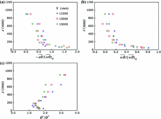
Profiles of heat flux and r.m.s. temperature fluctuations. Symbols as in a

References
Adaramola MS, Krogstad P-Å (2011) Experimental invetigation of wake effects on wind turbine performance. Renew Energy 36:2078–2086
Ainslie JF (1988) Calculating the flowfield in the wake of wind turbines. J Wind Eng Ind Aerodyn 27:213–224
Andre JC, Mahrt L (1982) The nocturnal surface inversion and influence of clear-air radiative cooling. J Atmos Sci 39:864–878
Arya SP (1988) Introduction to micrometeorology. Academic Press Inc., USA 307 pp
Barthelmie RJ, Frandsen ST, Rathmann O, Hansen K, Politis E, Prospathopoulos J, Schepers JG, Rados K, Cabazón D, Schlez W, Neubert A, Heath M (2011) Flow and wakes in large wind farms: final report for UpWind WP8. Risø report R-1765(EN), 255 pp
Beljaars ACM, Holtslag AAM (1991) Flux parameterisation over land surfaces for atmospheric models. J Appl Meteorol 30:327–341
Born M, Wolf E (1999) Principles of optics: electromagnetic theory of propagation, interference and diffraction of light. Cambridge University Press, UK 986 pp
Chamorro LP, Porté-Agel F (2010) Effects of thermal stability and incoming boundary layer flow characteristics on wind turbine wakes: a wind tunnel study. Boundary-Layer Meteorol 136:515–533
Duynkerke PG (1999) Turbulence, radiation and fog in Dutch stable boundary layers. Boundary-Layer Meteorol 90:447–477
Dyer AJ (1974) A review of flux profile relationships. Boundary-Layer Meteorol 7:363–372
ESDU (2001) Characteristics of atmospheric turbulence near the ground. Part II: single point data for strong winds (neutral atmosphere). ESDU 85020. Engineering Sciences Data Unit, London, UK, p 42
ESDU (2002) Strong winds in the atmospheric boundary layer. Part 1: hourly-mean wind speeds. ESDU 85026. Engineering Sciences Data Unit, London, UK, p 61
Euromech (2012) Wind energy and the impact of turbulence on the conversion process. Euromech 528, University of Oldenburg, Oldenburg
Hancock PE, Bradshaw P (1989) Turbulence structure of a boundary layer beneath a turbulent free stream. J Fluid Mech 205:45–76
Hancock PE, Pascheke F (2014) Wind tunnel simulation of the wake flow of a large wind turbine in a stable boundary layer: part 2, the wake flow. Boundary-Layer Meteorol (this issue)
Heist DK, Castro IP (1998) Combined laser-doppler and cold wire anemometry for turbulent heat flux measurement. Exp Fluids 24:375–381
Högström U (1988) Non-dimensional wind and temperature profiles in the atmospheric surface layer: a re-evaluation. Boundary-Layer Meteorol 42:55–78
Högström U (1996) Review of some basic characteristics of the atmospheric surface layer. Boundary-Layer Meteorol 78:215–246
Irwin HPAH (1981) The design of spires for wind stimulation. J Wind Eng Ind Aerodyn 7:361–366
Kaimal JC, Finnigan JJ (1994) Atmospheric boundary layer flows; their structure and measurement. Oxford University Press, UK 302 pp
Lu H, Porté-Agel F (2011) Large-eddy simulation of a very large wind farm in a stable atmospheric boundary layer. Phys Fluids 23:065101
Magnusson M, Smedman A-S (1994) Influence of atmospheric stability on wind turbine wakes. J Wind Eng 18:139–152
Magnusson M, Smedman A-S (1996) A practical method to estimate the wind turbine wake characteristics from turbine data and routine wind measurements. J Wind Eng 20:73–92
Marht L, Heald RC, Lenschow DH, Stankov BB, Troen IB (1979) An observational study of the structure of the nocturnal boundary layer. Boundary-Layer Meteorol 17:247–264
Mironov D, Fedorovich E (2010) On the limiting effect of the earth’s rotation in the depth of a stably stratified boundary layer. Q J R Meteorol Soc 136:1473–1480
Nieuwstadt FTM (1984) The turbulent structure of the stable, nocturnal boundary layer. J Atmos Sci 41:2202–2216
Ohya Y (2001) Wind-tunnel study of atmospheric stable boundary layers over a rough surface. Boundary-Layer Meteorol 98:57–82
Ohya Y, Uchida T (2003) Turbulence structure of stable boundary layers with a near-linear temperature profile. Boundary-Layer Meteorol 108:19–38
Resagk C, du Puits R, Thess A (2003) Error estimation of laser-Doppler anemometry measurements in fluids with spatial inhomogeneities of the refractive index. Exp Fluids 35:357–363
Sanderse B (2009) Aerodynamics of wind turbine wakes: literature review. Energy Research Centre of the Netherlands, Report ECN-E-09-016, 46 pp
Sanderse B, van der Pijl SP, Koren B (2011) Review of computational fluid dynamics for wind turbine wake aerodynamics. Wind Energy 14:799–819
Snyder WH, Castro IP (2002) The critical Reynolds number for roughwall boundary layers. J Wind Eng Ind Aerodyn 90:41–54
Stull RB (1988) An introduction to boundary layer meteorology. Kluwer Academic Publishers, Dordrecht 679 pp
Steeneveld GJ, van de Wiel BJH, Holtslag AAM (2007) Diagnostic equations for the stable boundary layer height: evaluation and dimensional analysis. J Appl Meteorol Climatol 46:212–225
Vermeer LJ, Sørensen JN, Crespo A (2003) Wind turbine wake aerodynamics. Progr Aerosp Sci 39:467–510
Zilitinkevich S, Calanca P (2000) An extended similarity theory for the stably stratified atmospheric boundary layer. Q J R Meteorol Soc 126:1913–1923
Acknowledgments
The work reported here was performed under SUPERGEN-Wind Phase 1, Engineering and Physical Sciences Research Council reference EP/D024566/1. Further details can be found from www.supergenwind.org.uk. The authors are particularly grateful to Dr P. Hayden for his assistance in setting up the experiments, and to Prof. A. G. Robins. The authors are also grateful to Prof. A. A. Holtslag (Univ. of Wageningen, Netherlands) for useful discussions regarding field measurements, and to a referee for drawing our attention to Resagk et al. (2003). The EnFlo wind tunnel is a Natural Environment Research Council/National Centre for Atmospheric Sciences (NCAS) national facility, and the authors are also grateful to NCAS for the support provided.
Author information
Authors and Affiliations
Corresponding author
Appendix: Effect of Temperature on LDA Measurements
Appendix: Effect of Temperature on LDA Measurements
The refractive index, \(n\), of air is dependent on temperature, and so the path of a constituent ray, and therefore that of a beam, may change. In a turbulent flow the path followed by a beam will vary along its length according to the variation of temperature with time along its length. As this is not known a simplified analysis is all that can be made. We follow the line of analysis set out by Resagk et al. (2003). If \(s\) is the distance along the ray from its origin at the probe lens, and \(\mathbf{\underline{r}}\) the position vector of a point along the ray then
(Born and Wolf 1999). The case of practical concern here is when the gradient is perpendicular to the ray direction, \(\xi \). Then, if \(\eta \) is the lateral displacement, this equation reduces to \(\hbox {d}^{2}\eta /\hbox {d}\xi ^{2}=(1/n) \hbox {d}n/\hbox {d}\eta \), and since the departure of \(n\) from unity is in any case small (see below), we obtain
say. Making the further assumptions that a focused beam can be represented by two rays converging at an angle of \(\pm \phi \) and that the gradient \(\beta \) is constant across the beam leads to the lateral displacement,\(\Delta \eta \), of the focus according to
where \(2 \delta \) is the beam separation at the lens and \(F\) is the distance to the focus. It can also be shown that the angle of the beam, \(\alpha \), at the focus is given by \(\beta F\).
Now, supposing the gradients are moderate enough for both beams (at small internal angle \(2 \Phi \)) to be affected equally, then Eq. 21 gives the lateral deflection of the measuring volume from the probe axis, and there is no movement along the probe axis. There is also no change in the angle between the beams and therefore no change in fringe spacing. Conversely, assuming the gradient across one beam is equal and opposite in magnitude to that across the other, leads to no lateral deflection of the measuring volume but does lead to a displacement from the probe according to
where \(\xi \) now denotes the distance along the probe axis, rather than along a beam. The change in beam internal angle is \(2\alpha \), and the fractional change in Doppler frequency \(\delta f/f=- \alpha /(\Phi +\alpha )\).
Now, taking \(\hbox {d}n/\hbox {d}T \approx 9.8 \times 10^{-7} \hbox { K}^{-1}\), and noting \(dT/d\eta \) has units Km\(^{-1}\), so that \(\beta = 9.8 \times 10^{-7}\) d \(T\) /d \(\eta \) (m\(^{-1}\)) and the probe parameters lead to \(\alpha =4.9\times 10^{-8}\;\hbox {d}T\hbox {/d}\eta ,\,\Delta \eta =1.2 \times 10^{-9}\;\hbox {d}T\hbox {/d}\eta \,(\hbox {m})\) and \(\Delta \xi =1.5\times 10^{-8}\;\hbox {d}T\hbox {/d}\eta \,(\hbox {m})\). From Fig. 7 \(\partial {\phi }'/\partial z\) is not larger than about \(3\hbox { K m}^{-1}\), so even if instantaneously \(\partial \phi (t)/\partial z\) was, say, three order of magnitude larger then, \(\alpha \approx 1.5 \times 10^{-4}\), and \(\Delta \eta \approx 3.7\, \upmu \hbox {m}\) and \(\Delta \xi \approx 46 \,\upmu \hbox {m}\), or about 3 % of the respective measuring volume dimensions. (If only one beam is supposed affected, then this fraction is about 1.5 %.) The fractional change in Doppler frequency is about 0.18 %. In conclusion, the effects of temperature fluctuations are expected to be negligible.
Rights and permissions
About this article
Cite this article
Hancock, P.E., Pascheke, F. Wind-Tunnel Simulation of the Wake of a Large Wind Turbine in a Stable Boundary Layer. Part 1: The Boundary-Layer Simulation. Boundary-Layer Meteorol 151, 3–21 (2014). https://doi.org/10.1007/s10546-013-9886-y
Received:
Accepted:
Published:
Issue Date:
DOI: https://doi.org/10.1007/s10546-013-9886-y