Turbulence Anisotropy in the Near-Surface Atmosphere and the Evaluation of Multiple Outer Length Scales

Abstract

Length scales determined by maximum turbulent kinetic energy (TKE), the integral scale, and two length scales based on Reynolds stress-tensor anisotropy are compared to the often stated outer length scales of boundary-layer depth and distance from the earth’s surface, $z$. The scales are calculated using sonic anemometer data from two elevations, 5 and 50 m above the ground at the main tower site of the CASES-99 field campaign. In general, none of these scales agrees with the other, although the scale of maximum TKE is often similar to the boundary-layer depth during daytime hours, and the length scales derived from anisotropy characteristics are sometimes similar to $\kappa \!z, z$, and $2z$ depending on scale definition and thermal stability. Except for the scale with the strictest isotropy threshold, the turbulence is anisotropic for each of the various candidates for the outer scale. Length scales for maximum buoyancy flux and temperature variance are evaluated and the turbulence characteristics at these scales are almost always found to be anisotropic.

1 Introduction

Turbulent motion of a fluid occurs over a broad range of scales. The smallest scales are usually defined as the scale at which the motion dissipates into heat due to the viscosity of the fluid. Most turbulence text books and turbulence applications use either the outer scale or integral scale as the term to describe the larger scales of turbulent motion (Hinze 1959; Tatarski 1961; Tennekes and Lumley 1972; Schlichting 1987; Gifford 1989; Kaimal and Finnigan 1994; Stull 1997). In this context, the outer scale is the largest scale of turbulence at the point of measurement, not to be confused with the outer-layer scale that is associated with the scales of turbulence far from the surface. The outer scale is variously defined as: on the order of the largest scale of the flow, the atmospheric boundary-layer depth; $\kappa \!z$ near the surface in the logarithmic layer; as the scale above which the Fourier transform no longer has a $-$5/3 slope; as the scale at which the structure function no longer follows a 2/3 power law, a very practical definition for optical applications. Turbulence at the outer scale is considered to be anything between the point at which the turbulence undergoes transition from isotropic to anisotropic to very anisotropic (Tatarski 1961). The outer scale is sometimes described as the scale at which the turbulent kinetic energy (TKE) is maximum. Or alternatively, near the surface (in the logarithmic layer or lowest 100 m), the outer scale is thought to grow linearly with height above the ground, $z$, and be roughly equal to $z$. Near a surface, boundary-layer theory uses $\kappa \!z$ as a typical eddy size at a distance $z$ from the surface based on Prandtl’s mixing length concept, where $\kappa$ is the von Karman constant.

A single book or paper will cite more than one of these definitions as synonymous or nearly so. Many measurements have been made to try to estimate the magnitude of the outer scale in the atmosphere. Estimates measured at high elevation observatories for astronomical applications are in the range of tens of metres (Ziad et al. 2004). Micrometeorological studies find outer scales on the order of hundreds to thousands of metres with considerable variation (Teunissen 1980; Kaimal and Finnigan 1994). With modern sonic anemometer data and innovative data processing, it is now possible to evaluate some of the relevant properties of atmospheric turbulence in a different way. One reason the issue of outer scale measurement has not been examined more extensively is that, for many situations, numerical model calculations are not highly sensitive to the actual value of the outer scale (Consortini et al. 1973). Given the broad range of applications, a single value or definition of outer scale is unlikely to be useful. More thorough knowledge of the properties of the various definitions should be of general use.

2 Data

The Cooperative Atmosphere–Surface Exchange Study (CASES-99) was a major field campaign located near Leon, Kansas, set up primarily to study the stable atmospheric boundary layer. The campaign took place in October 1999, and was centered around a heavily instrumented 60 m main tower site in flat terrain. In addition, there were six 10-m towers at a distance of 100 and 300 m from the main tower as well as other instrumentation (Poulos 2002). The main tower instruments recorded data continuously throughout the month, day and night. The CASES-99 dataset is available from the National Center for Atmospheric Research (NCAR) with quality control and tilt correction included http://www.eol.ucar.edu/projects/cases99/.

The data used here are from the Campbell Scientific CSAT3 sonic anemometers deployed at $z = 50$ m on the main tower and at $z = 5$ m on a shorter tower 10 m distance from the main tower. These sonic anemometers have a path length of 0.10 m, and all three paths share a common centre point. At the rate of 20 data points $\mathrm {s}^{-1}$, sonic anemometers can resolve scales only down to about 0.5 m at wind speeds typical of the CASES-99 experiment. This is nowhere near the scale of dissipation, $\sim$1 mm, but is adequate for examining the outer scale.

In addition to the three components of the wind vector, the CSAT3 sonics also record sonic temperature. The sonic temperature is derived from the speed of sound measurement that depends on both temperature and humidity. The temperature determined by sonic anemometers still includes the humidity dependence, $T_\mathrm{{s}}=T(1 + 0.51w)$, resulting in a temperature that is very close to the virtual temperature, $T_\mathrm{{v}}=T(1 + 0.61w)$, where $T$ is the dry-bulb temperature, $T_\mathrm{{s}}$ is the sonic temperature, $T_\mathrm{{v}}$ is the virtual temperature, and $w$ is the ratio of the water vapour mass to the total air mass (Campbell Scientific CSAT3 manual). A simple eddy-correlation calculation of the covariance of the sonic temperature and the vertical velocity is essentially the same as the buoyancy flux (Foken 2008).

Of the eight sonics on the main tower, only four are CSAT3 models. The four Applied Technologies ATI K sonic anemometers are configured such that the three transducer paths are separated by distances comparable to or larger than the path length of 0.15 m. As a result of the separation of the paths, the calculation of covariances at small spatial scales becomes problematic, so the data from the ATI K sonics are not used for this analysis. A more detailed analysis will also include data from the CSAT3 at 30 m and the fourth CSAT3, which was at $z = 1.5$ m for the first part of the field campaign and was moved to $z = 0.5$ m for the final 10 days.

3 Data Analysis Tools

3.1 Multiresolution Decomposition

The data processing method used here is a combination of decomposing the wind velocity and sonic temperature data into the fraction of variance or covariance resulting from motion at different scales, then evaluating the anisotropy characteristics of the resulting Reynolds-stress tensor at each scale. The decomposition is done using a multiresolution technique (Vickers and Mahrt 2003) on segments of $2^{16}$ data points (54.6 min) starting at the top of each hour. Multiresolution spectra are analogous to Fourier spectra, but are decomposed using step functions instead of sinusoids. The use of step functions maintains Reynolds-averaging compatibility.

The peak of a multiresolution spectrum occurs at a slightly different scale than a Fourier spectral peak for the same data because the multiresolution peak depends on the width of major events whereas Fourier decomposition depends on the periodicity of major events (Howell and Mahrt 1997). The evaluated scale of maximum energy differs slightly between Fourier analysis and a multiresolution analysis of the same data.

Multiresolution spectra are less noisy than Fourier spectra of the same data, but can be sensitive to slight shifts in the starting point of the analysis. For example, significant variations can occur in individual spectral values from analysis of data from 1500 to 1555 UTC and 1501 to 1556 UTC even if the data are relatively stationary. For stationary data the area under the spectral curves will be the same for the two starting points. Sensitivity to starting point is overcome by employing an oversampling routine that has the effect of averaging out the starting point sensitivity and further smoothes the multiresolution spectrum, thus making the identification of peaks straightforward in most cases (Howell and Mahrt 1997). Spectral peak locations determined without the smoothing from oversampling are within a factor of two of the locations determined with oversampling.

If the multiresolution decomposition results in a maximum TKE spectral value at the largest scale, this is taken as an indication of non-stationarity and that 1-h period of data is excluded from the analysis. The largest resolved scale of a multiresolution decomposition is also a comparison of the first half of the data to the second half. When the spectral maximum is at the largest scale, the variation from the first half of the data to the second half is larger than variations at any of the smaller scales, an indication of non-stationarity. Eliminating the non-stationary 1-h periods results in removing the hours with the most stable thermal stratification in which small-scale turbulent motions had almost decayed and large-scale meandering becomes dominant. These very stable flows require a separate analysis, and are of interest for their ability to transport toxins without significant mixing, which results in a narrow area of highly toxic concentrations instead of the broad area of diffuse concentration that transport models predict.

3.2 Anisotropy Analysis

To fully describe anisotropy, two parameters are needed, the degree of anisotropy and the axisymmetry of the variances (Choi and Lumley 2001). Both parameters represent a continuum of values rather than binary states. Anisotropy analysis starts with the scaled Reynolds-stress tensor, ${\overline{{u}'_i {u}'_j}}/q$, where the prime indicates the difference from the mean, the overbar indicates the average, the subscripts cover all three wind vector components, and $\text {TKE} = q/2 =1/2\Big ({\overline{u'u'}+\overline{v'v'}+\overline{w'w'}}\Big )$. The analysis takes advantage of the property that all $3\times 3$ tensors have only three independent invariants, noting that there are an infinite number of sets of three independent invariants. Choi and Lumley use a set of mathematically elegant invariants common to tensor analysis, whereas Banerjee et al. (2007) use the three eigenvalues as the three invariants. Any set of invariants can be mapped to another set, therefore the two methods are transformable from one to the other. The method of Banerjee et al. is preferable for practical applications because the eigenvalues of the Reynolds-stress tensor are the fundamental variances of the turbulence. For this analysis, only $C_{3}$, the degree of anisotropy as defined by Bannerjee et al. is used, where

$$\begin{aligned} C_3 = 3\lambda _\mathrm{{s}} \end{aligned}$$

(1)

with $\lambda _\mathrm{{s}}$ being the value of the smallest eigenvalue. $C_{3}$ values fall between 0 and 1. At perfect isotropy no direction is preferred, and $C_{3} = 1$ because all eigenvalues $=$ 1/3. At the other extreme, variance exists in only two dimensions, and $C_{3} = 0$ because one eigenvalue vanishes. Additional anisotropy analysis of the CASES-99 data can be found in Klipp (2010, 2012).

3.3 Integral Scale Analysis

The integral scale for each 1-h period of data is determined by calculating the autocorrelation of the streamwise wind component for different time lags, and the point at which the correlation crosses or reaches zero is used to calculate an integral scale. Because the integral scale is expected to be large, on the order of the depth of the boundary layer, each time lag evaluated is twice as long as the previous time lag in order to greatly reduce computational time. As a result, the integral length scale estimates are of a coarser resolution than the other length scale calculations. In spite of this coarse method, the resulting length scales are self consistent and compare well with the scales derived from maximum TKE.

This method of calculating integral scales has a problem noted by others, in that sometimes no zero crossing is found, and such 1-h periods are not included in the integral scale results. Different methods of computing the integral scale can result in different values (Teunissen 1980). Many authors provide little detail on the calculation of integral times, making comparisons difficult.

3.4 Conversion of Time Scale to Length Scale

The sonic anemometer data are in the form of time series, so all scale calculations result in time scales. These are converted into length scales by multiplying the time scale by the mean wind speed for that data segment, resulting in a variance-based length scale. Although the mental model of turbulence as eddies of various sizes is useful, it is difficult to obtain quantitative measurements of eddies in the atmosphere, whereas point sensors readily measure variances and covariances, making the use of a variance-based length scale appropriate. For the subset of length scales for which the assumptions of Taylor’s frozen turbulence hypothesis hold, the variance length scale can also be considered an eddy size. Using a single-point measurement may be a source of differences with other works based on correlations between physically separated instruments. Another source of difference will be between Eulerian-type analyses herein, and Lagrangian-type analyses in other works.

3.5 A Note About Data Categories and Thresholds

Normally atmospheric surface-layer data are separated into thermal stability classes based on dimensionless parameters such as $z/L$ where $L$ is the local Obukhov length. For this analysis, $z/L$ separation is not as successful at separating classes of length scales as is the use of basic day/night separation along with thresholds of wind speed or buoyancy flux. For the larger scales, a buoyancy-flux threshold is most successful in explaining the spread of the data. For the smaller scales based on anisotropy analysis, a wind-speed threshold is most successful. The anisotropy arises from the surface-induced wind shear, so a wind-speed threshold is not surprising. For the larger scales, buoyancy flux alone is a larger influence than the combination of buoyancy flux and surface stress found in $z/L=\left( {{-\kappa \!zg}/{\bar{{\theta }}_\mathrm{{v}}}}\right) \left( {{\overline{{w}'{\theta }'_\mathrm{{v}}}}/{u_*^3}}\right)$, where $\kappa$ is the von Karman constant, $g$ is the acceleration due to gravity, $\theta _\mathrm{{v}}$ is the virtual potential temperature, and $u_*^2 =\left( {\overline{{u}'{w}'}^{2}+\overline{{v}'{w}'}^{2}} \right) ^{1/2}$.

The buoyancy flux and wind-speed thresholds have been determined empirically based on values such that the multi-peaked histograms calculated using all 1-h periods of data can be explained as sums of single-peaked histograms (Figs. 1, 2, 5, and 6). Simple classes of day/night and above/below threshold more distinctly separate the histograms than do classes based on $z/L$. An attempt to successfully convert the buoyancy-flux and wind-speed thresholds into $z/L$ classes is prevented by significant overlap of $z/L$ values between the different buoyancy-flux and wind-speed classes. The following $z/L$ values are found:

• At $z = 5$ m at night, when the buoyancy flux values are $< -$0.025 K m $\mathrm {s}^{-1}$, the corresponding $z/L$ values fall in the single range $0 < z/L < 0.5$, and when nighttime buoyancy fluxes are $> -$0.025 K m $\mathrm {s}^{-1}$, the $z/L$ values fall in two ranges, $0 < z/L < 0.02$ and $0.3 < z/L < 10$, including significant overlap with the other buoyancy-flux data class. At $z = 50$ m the behaviour is similar: for buoyancy fluxes $< -$0.015 K m $\mathrm {s}^{-1}$, the single range is $0 < z/L < 3$ and for buoyancy fluxes $> -$0.015 K m $\mathrm {s}^{-1}$, the two ranges are 0 $< z/L < 0.1$ and $0.6 < z/L < 15$. During 1-h periods with buoyancy flux values less than the threshold, conditions are closer to neutral, whereas 1-h periods with buoyancy flux values greater than the threshold are more stable. The most stable conditions are not included due to lack of stationarity over 1-h segments.

  Fig. 1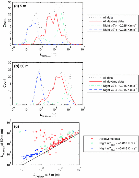

  

  Histograms of the length scale of maximum TKE, $L_\mathrm{{TKEmax}}$, for 1-h segments of data, at a $z = 5$ m and b $z=50$ m. Daytime $L_\mathrm{{TKEmax}}$ values are on the order of the boundary-layer depth, typically 1–3 km; near-neutral nighttime $L_\mathrm{{TKEmax}}$ values are smaller than the nocturnal boundary-layer depths of 500–800 m; whereas $L_\mathrm{{TKEmax}}$ values for more stable nighttime conditions are dominated by large-scale meandering motion. c Comparison of maximum TKE length scales at $z = 5$ m and $z = 50$ m, showing that the scale measured at $z = 50$ m is nearly always larger than the scale measured at $z = 5$ m but rarely by as much as a factor of 10. The black solid line is 1:1, black dotted indicates a factor of 2

  Fig. 2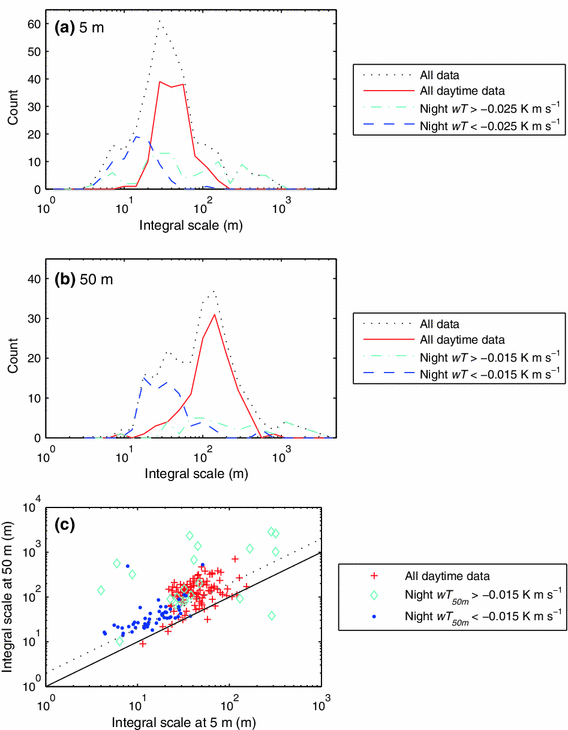

  

  Histograms of the integral length, for 1-h segments of data, at a $z = 5$ m and b $z = 50$ m. During the day the length scales are all less than the boundary-layer depth but significantly larger than the instrument height $z$, during near-neutral nighttime hours the scales are significantly smaller than the stable boundary-layer depth but mostly greater than the instrument elevation $z$; during more stable nighttime hours the length scales cover a broad range of values with no preferred length. c Comparison of integral scales at $z = 5$ m and $z = 50$ m, showing that the scale measured at $z = 50$ m is nearly always larger than the scale measured at $z = 5$ m. The black solid line is 1:1, black dotted indicates a factor of 3

• The wind-speed thresholds of 4.0 m $\mathrm {s}^{-1}$ at $z = 5$ and 9.0 m $\mathrm {s}^{-1}$ at $z = 50$ m are consistent with a logarithmic wind-speed profile. At $z = 5$ m, 1-h periods with wind speeds $>$4.0 m $\mathrm {s}^{-1}$ both day and night have $-0.4 < z/L < 0.15$, and periods with wind speeds $<$4 m $\mathrm {s}^{-1}$ have $-10.0 < z/L < 10.0$. Many of the 1-h periods with wind speeds $< 4$ m $\mathrm {s}^{-1}$ have $-0.4 < z/L < 0.15$, the same range as when wind speeds are $>$4.0 m $\mathrm {s}^{-1}$. Similarly at $z = 50$ m, 1-h periods with wind speeds $>$9.0 m $\mathrm {s}^{-1}$ have $-1.5 < z/L < 1.5$; periods with wind speeds $<$9.0 m $\mathrm {s}^{-1}$ have $-20 < z/L < 20$, including many periods with $-1.5 < z/L < 1.5$, the same range as periods with above threshold wind speeds. During high wind conditions, shear forces dominate day or night, whereas during light wind conditions, the thermal state dominates.

For the relatively flat grass-covered surface of the CASES-99 experiment site, high wind speeds are defined as $>$ 4.0 m $\mathrm {s}^{-1}$ at 5 m above the surface and $>$9.0 m $\mathrm {s}^{-1}$ at 50 m above the surface. These thresholds are determined empirically based on values that most effectively explain the multiple peaks of the data on the histograms in Figs. 5 and 6. Although this criterion results in fairly sharply defined thresholds, it is most probable that these thresholds are dependent on surface roughness and are not universal. Interestingly, Sun et al. (2012) arrive at very similar, and similarly sharply defined, wind-speed thresholds at $z = 5$ m and $z = 50$ m (3.0 and 8.5 m $\mathrm {s}^{-1}$ respectively) on the CASES-99 main tower even though they use only nighttime data, do not exclude the most stable conditions, and are comparing 10-min TKE values to 10-min mean wind speeds.

For this analysis, day is defined as 1400–2259 UTC and night as 0000–1359 and 2300–2359 UTC with solar noon at about 1815 UTC. Sunrise varies from 1230 to 1250 UTC and sunset from 2359 to 2330 over the course of the field campaign. These hours are included with the night data. Of the 600 possible 1-h periods of data 6–30 October, at $z = 5$ m 106 periods are missing some or all of the data, 170 1-h periods of data are flagged as non-stationary (defined in Sect. 3.1), leaving 324 1-h periods of data. At $z = 50$ m, 264 1-h periods are missing some or all of the data, 104 1-h periods are flagged as non-stationary, leaving 229 1-h periods of data. Table 1 contains details of the number of periods in each classification used in the analysis. As with any large field campaign, there are times when not all the instrumentation is operational, so plots comparing data from one sonic to data from the other sonic may show fewer data points than plots of each individual instrument’s data.

Fig. 3

The integral length scale plotted against the length scale of maximum TKE at a $z = 5$ m and b $z = 50$ m. The relationships $L_{\mathrm{int}} = 0.75\mathrm {L}_{\mathrm{TKEmax}}$ (dashed lines) and $L_{\mathrm{int}} = 0.33\mathrm {L}_{\mathrm{TKEmax}}$ (dotted lines) are shown

Fig. 4

Sample $C_{3}$ values, the degree of isotropy, for $z = 50$ m for the 1400–1459 UTC data for the 12 days with data that hour (solar noon is 1815 UTC). Locating the length scale at which $C_{3} = 0.5$ is usually less ambiguous than locating the scale at which the isotropic turbulence begins to become anisotropic

Table 1 Number of hours of data in each class and subclass in Figs. 1, 2, 3, 4, 5, 6, 7, 8, 9 , 10, and 11

Fig. 5

Histograms of $L_{\mathrm{half}}$, the length scale of transition from isotropic to anisotropic turbulence defined as $C_{3} = 0.5$, for 1-h segments of data, at a $z = 5$ m and b $z = 50$ m. During periods with high wind speeds, $L_\mathrm{{half}}$ values are between 1.5 and $2.5z$ with a peak near $2z$; during nighttime periods with low wind speeds, most $L_\mathrm{{half}}$ values at $z = 5$ m are in the range of $\kappa \!z$ to $z$, but values at $z = 50$ m are slightly smaller; during daytime periods with low wind speeds at $z = 5$ m, the values of $L_\mathrm{{half}}$ cover a broad range with no preferred scale, whereas at $z = 50$ m there is a broad peak at scales 100–1,000 m. Notable at $z = 5$ m are relatively few values of $L_{\mathrm{half}}=z$. c Comparison of $L_{\mathrm{half}}$ values at $z = 5$ m and $z = 50$ m. For nighttime hours of all wind speeds $L_{\mathrm{half}}$ at $z = 50$ m is about five times the value of $L_{\mathrm{half}}$ at $z = 5$ m. This relationship does not hold for daytime hours. The black solid line is 1:1, black dotted line indicates a factor of 5

4 Results

4.1 Maximum Turbulence Scales

One description of the outer scale of turbulence is that it encompasses the largest scale of motion possible in the system. For atmospheric flows, the largest scale is usually assumed to be on the order of the depth of the boundary layer. Another definition is that the outer scale is the scale with the most energy. Turbulent kinetic energy ($q/2$) is one half the sum of the wind-speed variances, $q/2 = \frac{1}{2}\left( {\overline{{u}'{u}'} + \overline{{v}'{v}'} + \overline{{w}'{w}'}}\right)$, and the maximum TKE scale is the scale at which the sum of the spectra of the variances is a maximum.

Histograms of the maximum TKE scale from each hour of relatively stationary data, $L_\mathrm{{TKEmax}}$, are shown in Fig. 1a and b. In the daytime, the boundary-layer depth is expected to be $\approx$1–2 km on most days of the experiment (Stull 1997) and the histograms for both instrument elevations encompass the 2-km scale near the daytime peak (solid lines). Because the boundary layer is growing and decaying during some of the hours defined as daytime, it might be expected that the daytime portion of the histogram would have a range encompassing a few hundred metres up to 2 or 3 km, the maximum boundary-layer depth, but a significant number of daytime hours show $L_\mathrm{{TKEmax}}$ at scales on the order of 10 km. These large $L_\mathrm{{TKEmax}}$ values are attributed to very large spectral values at large spatial scales for the lateral cross-stream component. A common occurrence in the presence of convection, these large-scale cross-stream spectral peaks dominate the TKE multiresolution spectrum (Klipp 2010). The scales for the cross-stream variance peaks are on the order of several to 10 km, or variances with time scales on the order of 7–20 min. These very large-scale motions may be comparable to surface-layer superstructures seen in very high Reynolds number turbulence in laboratory flows (Smits et al. 2011), but motion on this scale has been observed throughout the atmospheric boundary layer (Kropfli 1979) not just at the surface.

At night, the boundary-layer depths are on the order of several hundred metres for windier, weakly stable conditions. The sections of the histograms for the nighttime subset of the data are not consistent with the boundary-layer depth, showing peaks in the 10–70 m range for the $z = 5$ m sonic, and a 40–120 m range at $z = 50$ m (dashed lines, Fig. 1a, b). For the most stable conditions included in this analysis, the most common length scales are on the order of 2–5 km at $z = 5$ m and 5–12 km at $z = 50$ m (dash-dot lines, Fig. 1a, b). Under these weak turbulence conditions, motion at all scales is diminished compared to motion during more neutral conditions, but turbulent motion at the smaller and mid-sized scales diminishes more, resulting in more energy in large-scale meandering motion than in turbulent scales of motion.

From this, it can be concluded that $L_\mathrm{{TKEmax}}$ is somewhat comparable to the boundary-layer depth during the day but not at night. This conclusion is based on data from $z = 5$ m and $z = 50$ m from the surface, usually considered to be too close to the ground for eddies of the scale of the boundary-layer depth to exist due to the constraint of the solid surface. Whether or not eddies of this size exist close to the surface, motion with large variance-based length scales is readily observed near the surface.

Although $L_\mathrm{{TKEmax}}$ at both $z = 5$ m and $z = 50$ m is often measured to be on the order of the boundary-layer depth in the daytime, $L_\mathrm{{TKEmax}}$ values also depend on the height above the surface. If measured values of $L_\mathrm{{TKEmax}}$ were a function of only the boundary-layer depth, then a scatter plot of the values measured at $z = 50$ m plotted against the values measured at $z = 5$ m for the same 1-h periods should have the data clustered around a line with a 1:1 relationship (solid line, Fig. 1c). If the relationship were a simple linear dependence on $z$, then the scatter plot should have the data clustered around a line with a 10:1 relationship. The data in Fig. 1c cluster around a 2:1 line, so neither boundary-layer depth dependence nor $z$ dependence dominates the relationship. The data are closer to the 1:1 line than the 10:1 line indicating that boundary-layer depth dependence might have a larger influence than $z$ dependence.

Most of the daytime data (Fig. 1c) and more stable nighttime data cluster around the 2:1 relationship, but the near-neutral nighttime data appear to cluster around the line $L_\mathrm{{TKEmax}}$(50 m) $=$ (4/3) $L_\mathrm{{TKE}}$(5 m) $+$ 40. Given a lack of a theoretical basis for such a relationship, the appearance that the data lie around this line can be assumed to be a coincidence. The near-neutral data are also consistent with an interpretation of $L_\mathrm{{TKEmax}}$ at $z = 50$ m being 2–4 times the value at $z = 5$ m. Because this analysis compares data at only two heights above the surface, it cannot be determined whether the maximum TKE scale continues to increase with height above the surface or stays close to the magnitude of the boundary-layer depth.

4.2 Integral Scales

The histograms for the integral scales, $L_\mathrm{{int}}$, (Fig. 2a, b) show a separation into day and night behaviour similar to the $L_\mathrm{{TKEmax}}$ histograms but at smaller scales. The daytime peak at $z = 5$ m is in the 25–70 m range, and at $z = 50$ m the typical daytime length scales are on the order of 80–250 m. These scales do not approach the typical daytime boundary-layer depths on the order of km. Nighttime near-neutral scales are on the order of 6–25 m at $z = 5$ m and 15–60 m at $z = 50$ m. At both heights above the surface, the more stable nighttime portion of the histograms covers a broad range of integral scale lengths with no significant peaks.

Comparing the integral scale at $z = 5$ m to the scale at $z = 50$ m (Fig. 2c), the $z = 50$ m length scale is larger than the $z = 5$ m scale, with the 1:1 relationship indicated by a solid line. The integral scale at $z = 50$ m is roughly three times the integral scale measured at $z = 5$ m for the daytime data and near-neutral nighttime data. No relationship seems to exist between integral scales measured at the two heights above the surface for the more stable nighttime data.

Turbulence for the more stable 1-h periods is dominated by meandering motion as suggested by the very large scales of maximum TKE for these data (Fig. 1a, b). Although measured $L_\mathrm{{TKEmax}}$ show a 2:1 relationship between $z = 5$ m and $z = 50$ m (Fig. 1c), the integral scales, and therefore the underlying autocorrelations, of the meandering motion (Fig. 2c) do not share the same properties from one level to the next for the more stable 1-h periods. The lack of a significant peak in the histograms for the integral scales for the stable 1-h periods (Fig. 2a, b) is another indication that the autocorrelations of meandering motion behave differently than the autocorrelations typical of the stronger turbulence under near-neutral and daytime conditions.

4.3 Relationship Between Integral Scale and Maximum TKE Scale

Frehlich et al. (2008) report a relationship between the outer scale and integral scale of $L_\mathrm{{integral}} = 0.75L_\mathrm{{outer}}$ obtained from Hinze (1959). In Hinze, the outer scale is specifically the scale at which the Fourier transform is maximum, and the integral scale is assumed to be derived from the Fourier transform of the autocorrelation function. Based on the assumption of isotropy and a $-$5/3 power law in the inertial subrange, Hinze derives the relationship $L_\mathrm{{integral}} =\sqrt{\pi }\left( {\Gamma \!\left( {5/6}\right) }/{\Gamma \!\left( {1/3}\right) }\right) L_\mathrm{{outer}}$. In Fig. 3a and b, the integral scale is plotted against the length scale of maximum TKE for both heights above the surface. The relationship $L_\mathrm{{int}} = 0.75L_\mathrm{{TKEmax}}$ is indicated with a dashed line. Although few points lie along that line, it represents an upper bound for the relationship between the two scales at both heights above the surface, so $L_\mathrm{{TKEmax}}$ and $L_\mathrm{{int}}$ are not interchangeable. An empirical constant of proportionality of 0.33 is more representative of the near-neutral data, indicated by the dotted line. The near-neutral data have the least influence from thermal effects and are the most similar to the perfectly neutral stratification assumed in Hinze (1959). For the unstable 1-h segments and the more stable segments, no discernible relationship exists between $L_\mathrm{{int}}$ and $L_\mathrm{{TKEmax}}$.

Others have noted (i.e. Teunissen 1980) that integral lengths depend heavily on the method used to calculate the integral scale. A different method of calculating the integral scales might have a significant effect on the relationship between $L_\mathrm{{int}}$ and $L_\mathrm{{TKEmax}}$. The integral scales here are calculated based on the autocorrelation function (Sect. 3.3) and can be expected to vary significantly from the spectral method assumed by Hinze. Also, the maxima based on multiresolution spectra are known to have slightly different values than the maxima based on Fourier spectra (Sect. 3.1). These differences may be the only source of disagreement between the theoretical relationship $L_\mathrm{{int}} = 0.75L_\mathrm{{TKEmax}}$ and the empirical relationship $L_\mathrm{{int}} = 0.33L_\mathrm{{TKEmax}}$. The disagreement could also be attributed to Hinze’s assumption of isotropy, which does not apply to these larger scales.

4.4 Scales Separating Isotropic and Anisotropic Turbulent Motion

The length scale of maximum TKE is determined from the multiresolution spectral peaks and the integral scale is determined from wind-speed autocorrelation calculations. Neither method depends on evaluation of the anisotropy. By constructing Reynolds-stress tensors using the multiresolution spectra, the anisotropy of the motion at each spectral scale can be calculated as outlined in Sect. 3.2 by the method of Banerjee et al. (2007). Using this method, isotropic turbulence will have $C_{3} = 1.0$. The turbulence at the scales $L_\mathrm{{TKEmax}}$ and $L_\mathrm{{int}}$ is anisotropic because nearly all $C_{3}$ values for $L_\mathrm{{TKEmax}}$ are in the range of 0–0.3 at $z = 5$ m and 0–0.4 at $z = 50$ m and most $C_{3}$ values for $L_\mathrm{{int}}$ are in the range of 0.1–0.5 at $z = 5$ m and 0.4–0.7 at $z = 50$ m.

Although the $C_{3}$ spectrum for each 1-h period shows the expected general behaviour of being relatively isotropic at small scales and anisotropic at large scales, there are no scales at which $C_{3}$ reaches the value of pure isotropy (Fig. 4). With no scale having $C_{3} = 1.0$, locating a scale at which the flow starts to become anisotropic becomes problematic. The situation is further complicated by the smallest resolved scales appearing to be less isotropic than slightly larger scales. This might be attributed to turbulent motion, at scales too short to be resolved by the sonic anemometers, being aliased onto the smaller resolved scales, resulting in imprecise spectral magnitudes at the smallest pair of scales. Wind-speed data from other instrument types with small-scale resolution, such as hot-wire anemometers, will be needed to test if $C_{3} \ne 1.0$ is due to sonic anemometer limitations or if the flow never achieves strictly pure isotropy at any scale. Although it is assumed that turbulence reaches pure isotropy at small enough scale for all flows, some well respected experiments have contradicted this assumption (Pope 2000, p. 254; Casciola et al. 2007, and references therein).

Two different definitions of the scale of transition from isotropic to anisotropic turbulence are used herein. The first, $L_\mathrm{{half}}$, uses the point at which $C_{3}$ reaches the threshold of 0.5 as $C_{3}$ descends from high to low values. This threshold is arbitrary, but is relatively easy for an automated routine to locate.

The second scale, $L_\mathrm{{trans}}$, attempts to mimic the transition scale a human might choose by locating the point at which $C_{3}$ begins to significantly descend from its plateau value. The small sample of $C_{3}$ spectra in Fig. 4 hints at the complexity of many of the other $C_{3}$ spectra. The location on the plot at which a human eye will identify the transition is not usually near the maximum calculated by a computer. To approximate the scale a human might choose, the threshold of dropping below 90 % of the maximum $C_{3}$ for that hour is chosen. Varying the threshold used to calculate $L_\mathrm{{trans}}$ between 85–95 % results in subtle differences in the following results, but no qualitative changes in the conclusions. Periods in which $C_{3}$ never exceeds 0.5 are left out of the analyses.

The histograms of $L_\mathrm{{half}}$ values at $z = 5$ m and $z = 50$ m (Fig. 5a, b) indicate that for most of the periods with high wind speeds, day and night, $L_\mathrm{{half}}$ values are on the order of $2z$. For the periods with low wind speeds at night $L_\mathrm{{half}}$ values are comparable to $\kappa \!z$, whereas for the daytime periods with low wind speeds, $L_\mathrm{{half}}$ values cover a broad range of larger scales. It is notable that at $z = 5$ m, there is a relative lack of $L_\mathrm{{half}}$ values on the order of 5 m.

Knowledge of $L_\mathrm{{half}}$ at one level does not usually allow accurate prediction of $L_\mathrm{{half}}$ at the other level (Fig. 5c). For periods with high wind speeds, a relatively narrow range of $L_\mathrm{{half}}$ values at $z = 5$ m corresponds to a broader range of $L_\mathrm{{half}}$ values at $z = 50$ m, but dividing the periods with high wind speeds into day and night classes, most of the nighttime data have $L_\mathrm{{half}}$ values at $z = 50$ m, approximately 5 times the values measured at $z = 5$ m. Periods with low wind speeds have daytime values of $L_\mathrm{{half}}$ more than ten times larger at $z = 50$ m than at $z = 5$ m, whereas some of the periods with low wind speeds at night have $L_\mathrm{{half}}$ values widely scattered around the 1:1 line. If $L_\mathrm{{half}}$ were proportional to $z, \kappa \!z$, or $2z$, it would be expected that many of the points comparing $L_\mathrm{{half}}$ values at $z = 5$ m to those at $z = 50$ m would fall along a factor-of-10 line.

The characteristics of $L_\mathrm{{trans}}$ are similar to those for $L_\mathrm{{half}}$, but the scales are smaller, as expected from their definitions. At $z = 5$ m (Fig. 6a), the $L_\mathrm{{trans}}$ values for periods with high wind speeds fall mostly between 2 and 4.5 m. For nighttime periods with low wind speeds, $L_\mathrm{{trans}}$ values are between 0.25 and 1.75 m, whereas $L_\mathrm{{trans}}$ values for daytime periods with low wind speeds are between 2 and 6 m with no significant peak. Similar to the $L_\mathrm{{half}}$ analysis, $L_\mathrm{{trans}}$ length scales have a notable gap; at $z$ = 5 m few 1-h periods have $L_\mathrm{{trans}}$ length scales of $\kappa \!z$. At $z = 50$ m, $L_\mathrm{{trans}}$ values for periods with high wind speeds are between 5 and 40 m, for periods with low wind speeds at night, $L_\mathrm{{trans}}$ values are mostly $<$10 m, and for periods with low wind speeds during the day, $L_\mathrm{{trans}}$ values are between 5 and 300 m. Comparing $L_\mathrm{{trans}}$ at $z = 5$ m to $L_\mathrm{{trans}}$ at $z = 50$ m, the daytime data of any wind speed show no relationship between the two heights above the surface. The lack of correlation between $z = 5$ m and $z = 50$ m for both $L_\mathrm{{half}}$ and $L_\mathrm{{trans}}$ is an indication that buoyancy, in addition to shear, affects anisotropy. For the nocturnal data at any wind speed, the value measured at $z = 50$ m is three times the value at $z = 5$ m.

Fig. 6

Histograms of $L_{\mathrm{trans}}$, the length scale of transition from isotropic to anisotropic turbulence defined as $C_{3} = 0.9\; C_{\mathrm{3max}}$, for 1-h segments of data, at a $z=5$ m and b $z = 50$ m. For nighttime periods with low wind speeds, all $L_{\mathrm{trans}}$ values are $\kappa \!z$ or smaller; for periods with high wind speeds at $z = 5$ m, $L_{\mathrm{trans}}$ scales are between $\kappa \!z$ and $z$, whereas at $z = 50$ m, they are between $0.1z$ and $z$. The daytime values of $L_{\mathrm{trans}}$ for periods with low wind speeds cover a broad range. Notable at $z = 5$ m are relatively few values of $L_{\mathrm{trans}}=\kappa \!z$ or $L_{\mathrm{trans}}=z$. c Comparison of $L_{\mathrm{trans}}$ values at $z = 5$ m and $z = 50$ m. For nighttime segments of all wind speeds, $L_{\mathrm{trans}}$ at $z = 50$ m is about three times the value of $L_{\mathrm{trans}}$ at $z = 5$ m. This relationship does not hold for daytime segments. The black solid line is 1:1, black dotted line indicates a factor of 3

Classifying $L_\mathrm{{half}}$ and $L_\mathrm{{trans}}$ by day, night, and wind speed separates the multiple peaks in the total histograms at $z = 5$ m into sums of single peaks (Figs. 5a, 6a), but the peaks on the total histograms at $z = 50$ m (Figs. 5b, 6b) are more simply separated by only a day and night classification (Fig. 7). Daytime $L_\mathrm{{half}}$ values range from $2z$ to nearly the boundary-layer depth, nighttime values of $L_\mathrm{{half}}$ are $2z$ or less. $L_\mathrm{{trans}}$ values are slightly smaller with daytime values falling mostly between 10 and 100 m with a peak near $\kappa \!z = 20$ m, and nighttime $L_\mathrm{{trans}}$ values have a narrow peak at 5 m, with a range of 1–20 m.

Fig. 7

For $z = 50$ m, a histogram of $L_{\mathrm{half}}$ and b histogram of $L_{\mathrm{trans}}$. The distribution of data is well characterized by a simple day/night separation at $z = 50$ m without the additional classification by wind speed (Figs. 5b, 6b). During nighttime 1-h segments, $L_\mathrm{{half}}$ has a preferred length scale slightly larger than $\kappa \!z$ whereas all $L_{\mathrm{trans}}$ values are $< \kappa \!z$. For daytime 1-h segments, $L_{\mathrm{half}}$ values are mostly larger than $2z$ whereas $L_{\mathrm{trans}}$ includes a broad range of values mostly between $\kappa \!z$ and $2z$

The calculation of both $L_\mathrm{{half}}$ and $L_\mathrm{{trans}}$ depends on the anisotropy, and the two values correspond well with each other as a result. For $z = 5$ m, $L_\mathrm{{half}}$ and $L_\mathrm{{trans}}$ are well correlated with $L_\mathrm{{half}}$ values being 2–5 times larger than the corresponding $L_\mathrm{{trans}}$ value. At $z = 50$ m, $L_\mathrm{{half}}$ and $L_\mathrm{{trans}}$ are less well correlated, but most $L_\mathrm{{half}}$ values are within 3–10 times the corresponding $L_\mathrm{{trans}}$ value.

4.5 Relationship Between the Anisotropy Scales and the Integral Scale

The anisotropy-based scales are much smaller than the integral scales and $L_\mathrm{{TKEmax}}$. For most combinations, knowledge of one of the larger scales gives no information about the smaller ones and vice versa. One exception is the integral scale and $L_\mathrm{{half}}$ at $z = 50$ m. The total histogram curve for the integral scale at $z = 50$ m (dotted line, Fig. 2b) is very similar to the histogram curve for $L_\mathrm{{half}}$ at $z = 50$ m (dotted line, Fig. 5b) with a strong peak in the 100–200-m range and a secondary peak near 40 m. Plotting one scale versus the other (Fig. 8) shows no relationship between the integral scale and $L_\mathrm{{half}}$ for periods with low wind speeds, indicating that the similarity in the histograms is superficial. For periods with high wind speeds, however, the two length scales seem equivalent, mostly within a factor of two of each other, but given the scatter in the data, a relationship of $L_\mathrm{{half}} \propto \;(L_\mathrm{{int}})^{1/2}$ is also supported (power law with slope 1/2). Because these scales are derived by very different means, any relationship on the plot is probably the result of coincidence rather than any equivalence between the two scales. The lack of any relationship between the integral scale and $L_\mathrm{{half}}$ at $z = 5$ m further strengthens the suggestion that the relationship at $z = 50$ m is coincidental.

Fig. 8

The length scale of transition from isotropic to anisotropic turbulence defined as $C_{3}= 0.5, L_{\mathrm{half}}$, compared to the integral scale for $z = 50$ m data. The bulk of the high wind-speed data falls near the 1:1 line, within a factor of two. This relationship does not hold for the periods with low wind speeds, or for any data at $z = 5$ m (not shown)

4.6 Temperature Variance and Buoyancy Flux

In addition to the six components of the Reynolds-stress tensor, both the sonic temperature variance and the buoyancy flux can be calculated with sonic anemometer data. Fluxes and variances of scalar concentrations in the atmosphere are a direct result of the mechanical turbulence of the atmosphere. Although atmospheric turbulence drives the transport of scalars, the length scales discussed in the previous sections do not correspond directly to the scales of maximum buoyancy flux or maximum temperature variance.

During the day, the length scales of maximum buoyancy flux, $L_\mathrm{{WTmax}}$, at $z = 5$ m are mostly in the 10–100-m range and, at $z = 50$ m, most are in the 100–3,000-m range (Fig. 9), larger than $L_\mathrm{{trans}}$ and $L_\mathrm{{half}}$, comparable to and larger than the integral scale, smaller than $L_\mathrm{{TKEmax}}$, and anisotropic. Nighttime near-neutral values for $L_\mathrm{{WTmax}}$ are in the range of 7–30 m at $z = 5$ m and 30–150 m at $z = 50$ m, which are anisotropic because they are larger than the $L_\mathrm{{half}}$ and $L_\mathrm{{trans}}$ values for the same data class. The length scales for more stable nighttime conditions fall into two ranges, a small scale on the order of $z$, which is approximately isotropic, and a large scale of 1–10 km, larger than the nighttime boundary-layer depth. These meandering motion scales are anisotropic because they are larger than the scales derived from $C_{3}$.

Fig. 9

Histograms of the length scale of maximum buoyancy flux, $L_{\mathrm{WTmax}}$, for 1-h segments of data, at a $z = 5$ m and b $z = 50$ m. During the day, $L_{\mathrm{WTmax}}$ values are on the order of 40–100 m at $z = 5$ m and on the order of 200–2,000 m at $z = 50$ m; during near-neutral nighttime hours, $L_{\mathrm{WTmax}}$ values are mostly on the order of $2z$; during more stable nighttime hours, $L_{\mathrm{WTmax}}$ values split into two categories: small values on the order of $z$; and values larger than the nighttime boundary-layer depths, which are dominated by large-scale meandering motion

Peak sonic temperature-variance scales, $L_\mathrm{{TTmax}}$, in the daytime are mostly on the order of 40–600 m at $z = 5$ m and 100–4,000 m at $z = 50$ m (Fig. 10), slightly larger than the $L_\mathrm{{WTmax}}$ scales, but still smaller than $L_\mathrm{{TKEmax}}$. The near-neutral nighttime length scales are 10–70 m at $z = 5$ m, and 40–300 m at $z = 50$ m, also slightly larger than the $L_\mathrm{{WTmax}}$ scales, whereas the length scales under more stable conditions are almost all at the large meandering scales $>$1,000 m. For both heights above the surface, a non-negligible number of 1-h periods have peak temperature-variance scales at the smallest scales resolvable with the sonic anemometers, i.e. $<$2 m. It is probable that the actual peak scale is even smaller than these values. At $z = 5$ m, all these very small peak scales occur during two periods of cold-air advection, each approximately a day long, immediately following the passage of a cold front. These two events are also evident in the $z = 50$ m data. Very small peak scales are also evident in the $z = 50$ m data for several 1-h periods from other times of the month and may be caused by the presence of slightly cooler air above the tower. It is not yet known why the large-scale temperature variances should diminish so dramatically in these cases.

Fig. 10

Histograms of length scale of maximum temperature variance, $L_\mathrm{{TTmax}}$, for 1-h segments of data, at a $z = 5$ m and b $z = 50$ m. During the day, $L_\mathrm{{TTmax}}$ values are on the order of 60–300 m at $z = 5$ m and on the order of 300– 2,000 m at $z = 50$ m; during near-neutral nighttime hours, $L_\mathrm{{TTmax}}$ values are mostly on the order of 2–$4z$; during more stable nighttime hours, most $L_\mathrm{{TTmax}}$ values are at large scales dominated by large-scale meandering motion and some of the data have $L_\mathrm{{TTmax}} = 2z$. On the day following each of two frontal passages accompanied by cold-air advection, $L_\mathrm{{TTmax}}$ values are measured to be at the smallest scales resolvable with the sonic anemometers and include data from all three classes

Because temperature is a scalar, an analysis similar to the Reynolds stress-tensor anisotropy analysis is not possible. Instead, $L_\mathrm{{WTmax}}$ and $L_\mathrm{{TTmax}}$ are assigned the anisotropy of the Reynolds-stress tensor-derived $C_{3}$ for that scale. The $C_{3}$ values for peak buoyancy-flux scales and peak temperature-variance scales are found to collapse as a function of the non-dimensional length scales $L_\mathrm{{WTmax}}/L_\mathrm{{half}}$ and $L_\mathrm{{TTmax}}/L_\mathrm{{half}}$ (Fig. 11) at both heights above the surface. In both plots, for dimensionless length scales of 1.0 or greater, the data collapse well, but for dimensionless length $<$1.0, the data are disordered. This indicates that the dynamics of buoyancy flux and temperature variance at scales larger than $L_\mathrm{{half}}$ are dominated by the mechanical turbulence, which is anisotropic at these scales. At smaller scales of motion, the dynamics of buoyancy flux and temperature variance have an additional influence so scaling by $L_\mathrm{{half}}$ alone is not adequate to collapse the data onto a single curve. Viscous forces would be an obvious candidate to influence very small scales of buoyancy flux and temperature variance, but viscosity is not thought to be a significant factor at the scales resolvable by sonic anemometers.

Fig. 11

The anisotropy, $C_{3}$, for a $L_{\mathrm{WTmax}}$, the length scale of maximum buoyancy flux, and b $L_{\mathrm{TTmax}}$, the length scale of maximum temperature variance, as a function of non-dimensional length scale. The length scales $L_{\mathrm{WTmax}}$ and $L_{\mathrm{TTmax}}$ are made non-dimensional by dividing by the value of $L_{\mathrm{half}}$. The data collapse well for non-dimensional length scales $>$1.0. For non-dimensional length scales $<$1.0, the data are probably disordered even though the eye can find order in the relatively sparse data

5 Conclusions

Although the definition of the outer scale of turbulence that was used can often be inferred from the context of the publication and its field of study, greater clarity would be achieved by more specificity of which definitions and calculation methods were used and by knowing more about the turbulence properties at each of these scales. Since little relationship was found between the several definitions of outer scale examined in this analysis, the term outer scale should not be considered to simultaneously mean the largest scales of motion, the boundary-layer depth, and the integral scale. All the measures of outer scale evaluated here were anisotropic to some degree with $L_\mathrm{{trans}}$ being the closest to isotropic by definition.

Although the maximum TKE scale was sometimes on the order of the boundary-layer depth, this was only occasionally true during the day, whereas at night the maximum TKE scale was either much smaller than the boundary-layer depth or much larger depending on stability. Integral scales were in general slightly smaller than the maximum TKE scales but were not related to either boundary-layer depth or instrument height above the surface. The transition scale $L_\mathrm{{half}}$ appeared to be a reasonable candidate for a Prandtl mixing length, $\kappa \!z$, especially for periods with light winds at night. The transition scale $L_\mathrm{{trans}}$ appeared to be a candidate for an outer scale of practical use for optical applications based in part on its similarity to published optical outer scale values of 10–30 m (Ziad et al. 2004). Estimates of optical outer scales are based on the magnitude of temperature variance, but the scales of maximum temperature variance were not related to any of the outer scales of the mechanical turbulence.

Many definitions of outer scale in the surface layer include the height above the surface as an important parameter. Most of the evaluated scales in this analysis showed some degree of the influence of instrument height, but the relationship between values at $z = 5$ m and values at $z = 50$ m was not strong enough to support a purely linear relationship. In a few cases there was no correlation between a measured value at $z = 5$ m and the same measurement at $z = 50$ m—notably the integral scales under more stable conditions in which meandering motion dominates, and all the daytime data for the anisotropy-derived length scales, $L_\mathrm{{half}}$ and $L_\mathrm{{trans}}$.

Use of this analysis technique is new and leads to other areas of investigation. Can this method be used to learn more about how meandering motion differs from turbulent motion? Can thermal effects be separated from shear effects so as to study them independently, even though they usually occur simultaneously in the atmosphere? Why does the peak temperature-variance scale become very small with cold-air advection? Do other scalars have peak flux and variance scales in common with temperature?

References

Banerjee S, Krahl R, Durst F, Zenger Ch (2007) Presentation of anisotropy properties of turbulence, invariants versus eigenvalue approaches. J Turbul 8(32):1–27. doi:10.1080/14685240701506896
Casciola CM, Gualtieri P, Jacob B, Piva R (2007) The residual anisotropy at small scales in high shear turbulence. Phys Fluids 19:101704
Choi K-S, Lumley JL (2001) The return to isotropy of homogeneous turbulence. J Fluid Mech 436:59–84
Consortini A, Ronchi L, Moroder E (1973) Role of the outer scale of turbulence in atmospheric degradation of optical images. J Opt Soc Am 63:1246–1248
Foken T (2008) Micrometeorology. Springer-Verlag, Berlin, 306 pp
Frehlich R, Sharman R, Clough C, Padovani M, Fling K, Boughers W, Walton WS (2008) Effects of atmospheric turbulence on ballistic testing. J Appl Meteorol Clim 47:1539–1549
Gifford FA (1989) Does atmospheric turbulence have an outer scale? Agric For Meteorol 47:155–161
Hinze JO (1959) Turbulence: an introduction to its mechanism and theory. McGraw-Hill, New York, 586 pp
Howell JF, Mahrt L (1997) Multiresolution flux decomposition. Boundary-Layer Meteorol 83:117–137
Kaimal JC, Finnigan JJ (1994) Atmospheric boundary layer flows: their structure and measurement. Oxford University Press, New York, 289 p
Klipp C (2010) Near-surface anisotropic turbulence. Proc SPIE 7685:768505
Klipp C (2012) Near-surface turbulent temperature variances at multiple scales of motion. Proc SPIE 8380:838015
Kropfli RA (1979) PHOENIX multiple Doppler radar operations. In Hooke WH (ed) Project PHOENIX: the september 1978 field operation. NOAA/NCAR, Boulder. Digitized by the Internet Archive (2012), 281 pp. http://archive.org/details/projectphoenixse00hook. Accessed 5 Dec 2013
Pope SB (2000) Turbulent flows. Cambridge University Press, New York, 771 pp
Poulos GS et al (2002) CASES-99: a comprehensive investigation of the stable nocturnal boundary layer. Bull Am Meteorol Soc 83:555–581
Schlichting H (1987) Boundary-layer theory, 7th edn. McGraw-Hill, New York, 817 pp; J Kestin, translator
Smits AJ, McKeon BJ, Marusic I (2011) High-Reynolds number wall turbulence. Annu Rev Fluid Mech 43:353–375
Stull RB (1997) An introduction to boundary layer meteorology. Kluwer, Norwell, 670 pp
Sun J, Mahrt L, Banta RM, Pichugina YL (2012) Turbulence regimes and turbulence intermittency in the stable boundary layer during CASES-99. J Atmos Sci 69:338–351. doi:10.1175/JAS-D-11-082.1
Tatarski VI (1961) Wave propagation in a turbulent medium. McGraw-Hill, New York, 285 p; RA Silverman, translator
Tennekes H, Lumley JL (1972) A first course in turbulence. MIT Press, Cambridge, 300 pp
Teunissen HW (1980) Structure of mean winds and turbulence in the planetary boundary layer over rural terrain. Boundary-Layer Meteorol 19:187–221
Vickers D, Mahrt L (2003) The cospectral gap and turbulent flux calculations. J Atmos Ocean Technol 20:660–672
Ziad A, Schöck M, Chanan GA, Troy M, Dekany R, Lane BF, Borgnino J, Martin F (2004) Comparison of measurements of the outer scale of turbulence by three different techniques. Appl Opt 43:2316–2324
Acknowledgments
Thanks to Dr. Jiang Liu and Mr. David Tofsted of ARL for their helpful reviews. Thanks to the anonymous reviewers and the editor for the many questions and constructive comments. Thanks to the many participants of CASES-99 for the data which continue to yield new insights. CASES-99 data were provided by NCAR/EOL under sponsorship of the National Science Foundation. http://data.eol.ucar.edu/.
Author information
Authors and Affiliations
Corresponding author
Rights and permissions
Open Access This article is distributed under the terms of the Creative Commons Attribution License which permits any use, distribution, and reproduction in any medium, provided the original author(s) and the source are credited.
About this article
Cite this article
Klipp, C. Turbulence Anisotropy in the Near-Surface Atmosphere and the Evaluation of Multiple Outer Length Scales. Boundary-Layer Meteorol 151, 57–77 (2014). https://doi.org/10.1007/s10546-013-9884-0
Received:
Accepted:
Published:
Issue Date:
DOI: https://doi.org/10.1007/s10546-013-9884-0