Construction of Rosenbrock–Wanner method Rodas5P and numerical benchmarks within the Julia Differential Equations package

Abstract

Rosenbrock–Wanner methods for systems of stiff ordinary differential equations are well known since the seventies. They have been continuously developed and are efficient for differential-algebraic equations of index-1, as well. Their disadvantage that the Jacobian matrix has to be updated in every time step becomes more and more obsolete when automatic differentiation is used. Especially the family of Rodas methods has proven to be a standard in the Julia package DifferentialEquations. However, the fifth-order Rodas5 method undergoes order reduction for certain problem classes. Therefore, the goal of this paper is to compute a new set of coefficients for Rodas5 such that this order reduction is reduced. The procedure is similar to the derivation of the methods Rodas4P and Rodas4P2. In addition, it is possible to provide new dense output formulas for Rodas5 and the new method Rodas5P. Numerical tests show that for higher accuracy requirements Rodas5P always belongs to the best methods within the Rodas family.

1 The Rodas family in Julia DifferentialEquations package

Numerical programming in Julia has proven to be very performant. Rackauckas and Nie [16] implemented the powerful package |DifferentialEquations.jl| that contains a wide range of solvers for several types of problems. We restrict our considerations to initial value problems of the type

$$\begin{aligned} M \, y' = f(t,y), \; y(t_0)=y_0 \,. \end{aligned}$$

(1.1)

When matrix M is singular, (1.1) is a system of differential-algebraic equations (DAEs), else a system of ordinary differential equations (ODEs). We assume problem (1.1) to be of index not greater than one. For a detailed definition of the index concept see [7]. For solving such problems Rosenbrock–Wanner (ROW) methods are well known, see [4] and [8] for a recent survey.

A ROW scheme with stage-number s for problem (1.1) is defined by:

$$\begin{aligned} (M - h \, \gamma \, f_y) k_i{} & {} = {} h f \left( t_0+ \alpha _i h, y_0 + \sum _{j=1}^{i-1} \alpha _{ij} k_j \right) + h \, f_y \sum _{j=1}^{i-1} \gamma _{ij} k_j + h^2 \gamma _i f_t,\nonumber \\{} & {} \qquad i=1,...,s, \end{aligned}$$

(1.2)

$$\begin{aligned} y_1{} & {} = {} y_0 + \sum _{i=1}^{s} b_i k_i,\nonumber \\ \text { with } \quad f_y={} & {} {} \frac{\partial f}{\partial y}(t_0,y_0), \quad f_t = \frac{\partial f}{\partial t}(t_0,y_0). \end{aligned}$$

(1.3)

h is the stepsize and $y_1$ is the approximation of the solution $y(t_0+h)$. The coefficients of the method are $\gamma$, $\alpha _{ij}$, $\gamma _{ij}$, and $b_i$ define the weights. Moreover, it holds $\alpha _i = \sum _{j=1}^{i-1} \alpha _{ij}$ and $\gamma _i = \gamma + \sum _{j=1}^{i-1} \gamma _{ij}$.

ROW methods are alinearly implicit schemes since only a fixed number of s linear systems have to be solved. The index-1 condition guarantees the regularity of the matrix $(M - h \, \gamma \, f_y)$ for sufficiently small stepsizes $h >0$, see [4]. A disadvantage compared to implicit Runge–Kutta methods is the requirement of evaluating the Jacobian matrix $f_y$ in every timestep.

Within the Julia package |DifferentialEquations.jl| it is possible to compute the Jacobian by automatic differentiation. Therefore, ROW methods proved to be very efficient for the solution of stiff ODEs and DAEs. For the following analysis we choose |ROS3P| [10], |Rodas3| [21], |Rodas4| [4], |Rodas4P| [24], |Rodas4P2| [25] and |Rodas5| [3] from the many implemented ROW methods.

Moreover, we include |Ros3prl2| and |Rodas4PR2| [17] which are successors of |ROS3P| respectively |Ros3PL| [9] and |Rodas4P|, but not yet implemented in |DifferentialEquations.jl|. These schemes are applicable to index-1 DAEs and are stiffly stable. Stiffly stable methods guarantee $R(\infty )=0$ for the stability function R(z), which is a desired property when solving problem (1.1), see [4, 8]. Since in addition all these methods are A-stable they are L-stable as well. The best known method is certainly |Rodas4| from Hairer and Wanner [4]. The other schemes considered here were constructed based on this inspiration.

It is well known that ROW methods suffer from order reduction when they are applied to the Prothero-Robinson model, see [15, 18, 23]:

$$\begin{aligned} y' = \lambda \, (y-g(t))+g'(t), \quad y(0)=g(0). \end{aligned}$$

(1.4)

For a large stiffness parameter $|\lambda |$ with $\Re (\lambda )<<0$ the order may even drop to one. Scholz [23] and Ostermann and Roche [14] derived additional conditions to be fullfilled such that the order is independent on $\lambda$. Ostermann and Roche pointed out that the same conditions occur when semi-discretized parabolic partial differential equations (PDEs) are considered. Methods |ROS3P|, |ROS3PL|, |Ros3prl2|, |Rodas4P|, |Rodas4PR2| and |Rodas4P2| were developed according to these additional conditions. The letter P stands for “Prothero-Robinson” as well as “parabolic problem”.

An alternative way to avoid order reduction is considered in [1, 2]. Here, the method does not have to fulfill any additional order conditions. In order to achieve a higher stage order, adapted boundary conditions of the partial differential equation are considered in the calculation of the individual stages. The advantage is that every ROW method is suitable for this. The disadvantage is that additional information about the problem to be solved must be included in the stage evaluation. This may become complicated when pipe networks are considered and thus the boundary conditions must take coupling information into account [26]. A numerical comparison of the two approaches is given in Sect. 4.

W methods for ODEs are ROW methods which do not need an exact Jacobian matrix $f_y$ in every timestep. Examples for such methods can be found in [17]. Recently, Jax [5] was able to enlarge the class of certain W methods to problems of differential algebraic equations. Unfortunately a huge amount of additional order conditions have to be satiesfied as well. Conditions up to order two are fullfilled by the |Rodas4P2| method.

Table 1 summarizes the properties of the schemes considered. The order of convergence for some test problems was obtained numerically by the solution with different constant timesteps. The definition of the test problems is given in Sect. 4. Despite the fact that |Rodas4| and |Rodas5| are very efficient for a couple of typical test problems [4], they show remarkable order reduction for special problems.

Table 1 Stages s and order of convergence for different problems: Index-1 DAE problem (DAE-1), Prothero-Robinson model (Prot-Rob), parabolic problem (Parabol), index-2 DAE problem (DAE-2), DAE problem with inexact Jacobian (inexact Jac)

|Rodas5| has some further disadvantages. For simple non-autonomous problems such as $y' = \cos (t)$, $y(0)=0$, errors of this method and its embedded scheme are exactly the same. This leads to a failure of the stepsize control. The embedded method of |Rodas5| is not A-stable. In Fig. 1 we can see that the stability domain does not contain the whole left complex half-plane. This may cause stepsize reductions for problems with eigenvalues near the imaginary axis. Moreover, the original literature [3] does not contain a coefficient set for a dense output formula of |Rodas5|. In the Julia implementation a Hermite interpolation is used which is only applicable to ODE problems.

Fig. 1

Values $z \in {\mathbb {C}}$ with stability function $|R(z)|=1$, black for Rodas5, blue for its embedded method (colour figure online)

The aim of this paper therefore is to construct a new coefficient set for |Rodas5|. It should still have order 5(4) for standard DAE problems of index-1, but its order reduction shown in Table 1 should be restricted to that of |Rodas4P2|. Moreover, the embedded method should be A-stable and a dense output at least of order $p=4$ should be provided. In Sect. 2, all order conditions to be fullfilled by the new method |Rodas5P| are stated. The construction and the computation of the coefficients of the method is explained in Sect. 3, and finally, in Sect. 4, some numerical benchmarks are given.

2 Order conditions

The order conditions for Rosenbrock methods applied to index-1 DAEs of type (1.1) were derived by Roche [20]. They are connected to Butcher trees, as shown in Tables 2 and 3. Table 2 lists the conditions up to order $p=5$ for ODE problems and Table 3 the additional order conditions up to order $p=5$ for index-1 DAE problems, see [3, 4].

Table 2 Order conditions up to order $p=5$ for ODE problems

Table 3 Additional order conditions up to order $p=5$ for index-1 DAE problems

The following abbreviations are used:

$$\begin{aligned}{} & {} \beta _{i j} = \alpha _{i j} + \gamma _{i j} \, \; \text{ with } \quad \beta _{i j} = 0 \ \text{ for } \; i < j \ \text{ and } \ \beta _{ii}=\gamma _{i i}=\gamma , \end{aligned}$$

(2.1)

$$\begin{aligned}{} & {} \beta _i = \sum _{j=1}^{i}\beta _{i j} \, \quad \alpha _i = \sum _{j=1}^{i-1}\alpha _{i j}, \quad B = (\beta _{ i j})_{i,j=1}^{s} \, \quad W = B^{-1} = (w_{i j})_{i,j=1}^{s}.\qquad \end{aligned}$$

(2.2)

The sums in the tables are formed over all possible indices.

Table 4 Additional order conditions

In Table 4 additional order conditions are defined. Conditions No. 41–44 are given in [11] for problems of type $M(y) \cdot y' = f(y)$ with singular matrix M(y). Based on these conditions the method |rowdaind2| was derived in [11]. In the special case of index-2 DAEs of type

$$\begin{aligned} y'= & {} f(y,z), \end{aligned}$$

(2.3)

$$\begin{aligned} 0= & {} g(y) \end{aligned}$$

(2.4)

with a non-singular matrix $(\frac{\partial g}{\partial y} \cdot \frac{\partial f}{\partial z})$ in the neighborhood of the solution, condition No. 41 guarantees convergence order $p=2$. The additonal conditions No. 42–44 lead to order $p=3$ for the differential variable y and $p=2$ for the algebraic variable z of such index-2 problems.

Conditions No. 45–47 are introduced by Jax [5]. By these conditions at least order $p=2$ is achieved for index-1 problems using inexact Jacobian matrices. Method |Rodas4P2| has been derived for that purpose, see [25]. When the Jacobian is computed by finite differences, this property might be advantageous.

Conditions No. 48, 49 are necessary for the Prothero-Robinson model, see equation (1.4). The coefficients of polynomials $C_2(H)$ and $C_3(H)$ with $H = \frac{z}{1-\gamma z}$ and $z = \lambda \, h$ are defined according to [23]

$$\begin{aligned} A_0= & {} -N^{(2)}(-1) + \gamma M(-1)+M(0) \end{aligned}$$

(2.5)

$$\begin{aligned} A_i= & {} -N^{(2)}(i-1)+2\gamma M(i-1) + \gamma ^2 M(i-2)+M(i) \end{aligned}$$

(2.6)

$$\begin{aligned}{} & {} \quad \quad \quad \text{ for } \ 0<i<s \nonumber \\ A_s= & {} \gamma ^2 M(s-2) \end{aligned}$$

(2.7)

$$\begin{aligned}{} & {} \nonumber \\ B_0= & {} -N^{(3)}(-1)+N^{(2)}(0) \end{aligned}$$

(2.8)

$$\begin{aligned} B_i= & {} -N^{(3)}(i-1) +\gamma N^{(2)}(i-1)+ N^{(2)}(i) \end{aligned}$$

(2.9)

$$\begin{aligned}{} & {} \quad \quad \quad \text{ for } 0<i<s-1 \nonumber \\ B_{s-1}= & {} -N^{(3)}(s-2)+\gamma N^{(2)}(s-2) \end{aligned}$$

(2.10)

$$\begin{aligned} M(\nu )= & {} \sum _{i=1}^{s} b_i M_i(\nu ),\quad N^{(\sigma )}(\nu )=\sum _{i=1}^{s}b_i N_i^{(\sigma )}(\nu ) \quad \text{ for } \ \sigma \ge 2 \end{aligned}$$

(2.11)

with

$$\begin{aligned} M_i(\nu )= & {} \left\{ \begin{array}{lll} 1 \quad &{}\text{ if } &{} \nu < 0 \\ \beta _i' \quad &{}\text{ if } &{} \nu =0 \\ \sum \beta _{i j_1} \beta _{j_1 j_2} \ldots \beta _{j_{\nu -1}j_{\nu }} \beta _{j_{\nu }}' \quad &{}\text{ if } &{} \nu =1,\ldots ,i-2 \\ 0 \quad &{}\text{ if } &{} \nu \ge i-1 \end{array} \right. \end{aligned}$$

(2.12)

$$\begin{aligned} \sigma ! N_i^{(\sigma )}(\nu )= & {} \left\{ \begin{array}{lll} 1 \quad &{}\text{ if } &{} \nu < 0 \\ \alpha _i^{\sigma } \quad &{}\text{ if } &{} \nu =0 \\ \sum \beta _{i j_1} \beta _{j_1 j_2} \ldots \beta _{j_{\nu -1}j_{\nu }} \alpha _{j_{\nu }}^{\sigma } \quad &{}\text{ if } &{} \nu =1,\ldots ,i-2 \\ 0 \quad &{}\text{ if } &{} \nu \ge i-1 \end{array} \right. \end{aligned}$$

(2.13)

and $\beta _i' = \sum _{j=1}^{i-1}\beta _{i j}$. The summation in (2.12), (2.13) is over $j_\nu< \cdots< j_1 < i$. To distinguish summation $\sum _{j=1}^{i-1}\beta _{i j}$ and $\sum _{j=1}^{i}\beta _{i j}$ in the following, we introduce $\beta _{i j}'$ with $\beta _{i j}'=\beta _{i j}$ for $j<i$ and $\beta _{i j}'=0$ for $j \ge i$.

In order to fulfill conditions No. 48 and 49 in Table 4 all coefficients $A_i$ and $B_i$ must be zero. As stated in [25], the estimation of the error constant C of the global error in the paper of Scholz [23] is not sharp. It behaves like $C=\frac{1}{z}C_1$ for L-stable methods, see [17]. Therefore, for fixed h asymptotically exact results are obtained for $|\lambda | \rightarrow \infty$, but for fixed large stiffness $| \lambda |$ only order $p-1$ is obtained numerically. This can be seen in Table 1. Although the |Rodas4P| and |Rodas4P2| methods satisfy both conditions No. 48 and 49 they only show order $p=3$ for the Prothero-Robinson model with large stiffness $| \lambda |$, whereas |Rodas4PR2| achieves the full order in stiff case.

An L-stable method is obtained, when $|R(z)|<1$ for $\Re (z)<0$ and $R(\infty )=0$ holds. The stability function R(z) can be expressed in terms of $M(\nu )$ defined in (2.11) as follows

$$\begin{aligned} R(z) = \sum _{i=0}^s M(i-2) H^i. \end{aligned}$$

(2.14)

3 Construction of Rodas5P

The aim is to construct a method which fullfills all order conditions stated in Tables 2, 3 and 4. Analogously to [3], we choose $s=8$ and want to construct a stiffly accurate method with

$$\begin{aligned} b_i=\beta _{8 i} \quad \text{ for } i=1,\ldots ,7, \quad b_8=\gamma , \quad \alpha _8=1. \end{aligned}$$

(3.1)

The embedded method with stage number ${\hat{s}}=7$ is stiffly accurate, too:

$$\begin{aligned} {\hat{b}}_i=\beta _{7 i} \quad \text{ for } i=1,\ldots ,6, \quad {\hat{b}}_{7}=\gamma , \quad \alpha _{7}=1 . \end{aligned}$$

(3.2)

It should fullfill the order conditions No. 1-8, 18-22, 41, 48 leading to a method of order ${\hat{p}} = 4$ for index-1 DAEs. These conditions are denoted by ${\hat{1}}$, ${\hat{2}}$,...,$\hat{48}$.

According to [3, 4] we require

$$\begin{aligned} \alpha _{8 i}=\beta _{7 i} \quad \text{ for } i=1,\ldots ,7; \quad \alpha _{7 i}=\beta _{6 i} \quad \text{ for } i{=}1,\ldots ,6; \quad \alpha _6 {=} 1. \end{aligned}$$

(3.3)

Therefore, the following 40 coefficients remain to be determined:

$$\begin{aligned}{} & {} \gamma , \beta _{21}, \beta _{31},\beta _{32},...,\beta _{54},\beta _{62},...,\beta _{65},\beta _{72},...,\beta _{76},\beta _{82},...,\beta _{87},\\{} & {} \alpha _{21},\alpha _{31},\alpha _{32},\alpha _{41},\alpha _{42},\alpha _{43},\alpha _{51},\alpha _{52},\alpha _{53},\alpha _{54},\alpha _{62},\alpha _{63},\alpha _{64},\alpha _{65}. \end{aligned}$$

Coefficients $\beta _{61}$, $\beta _{71}$, $\beta _{81}$, $\alpha _{61}$ are not listed, since they are determined later by $\alpha _6=1$ and $\beta _8'=\beta _7'=\beta _6'=1-\gamma$, which follows from condition No.1 and the choice $\alpha _7=\alpha _8=1$.

Our strategy is to fulfill the conditions No. 48, 49 first. In these conditions occur terms belonging to the long trees (see conditions No. 1, 2, 4, 8, 17) and the trees belonging to conditions No. 3, 7, 16. Moreover, we try to fullfill at least some of the conditions to arrive at $C_4(H)=0$ where terms belonging to trees of conditions No. 5, 14 occur.

Moreover, we can simplify many conditions related to long trees. To give an example we reformulate conditions No. 2, 4:

$$\begin{aligned} \sum b_i \beta _{i}= & {} \frac{1}{2} \; \Leftrightarrow \\ \sum \beta _{8i}' \beta _i' + \gamma ^2 + 2 \gamma \beta _8'= & {} \frac{1}{2} \; \Leftrightarrow \\ \sum \beta _{8i}' \beta _i'= & {} \frac{1}{2} {-} \gamma ^2 {-} 2 \gamma (1{-}\gamma ) {=} \frac{1}{2}{-}2\gamma {+}\gamma ^2 \\ \sum b_i \beta _{ij} \beta _j= & {} \frac{1}{6} \; \Leftrightarrow \\ \sum \beta _{8i}' \beta _{ij}'\beta _j' + \gamma ^3 + 3 \gamma ^2 \beta _{8}' + 3 \gamma \sum \beta _{8i}'\beta _i'= & {} \frac{1}{6} \; \Leftrightarrow \\ \sum \beta _{8i}' \beta _{ij}'\beta _j'= & {} \frac{1}{6} {-}3\gamma \left( \frac{1}{2}{-}2\gamma {+}\gamma ^2 \right) {-}3 \gamma ^2 (1{-}\gamma ) {-} \gamma ^3 \\= & {} \frac{1}{6} - \frac{3}{2} \gamma + 3\gamma ^2 - \gamma ^3 \end{aligned}$$

• 1. In the first step we set $\alpha _{21}=3 \gamma$ and $\beta _{21}=0$, see [24]. By this choice the following conditions are fullfilled: No. 18, $\hat{18}$, 20, $\hat{20}$, 30, 47. Form No. 48, 49 we obtain $A_8=0$, ${\hat{A}}_7=0$, $B_7=0$.

• 2. Now we interpret $\gamma$, $\alpha _3$, $\alpha _4$, $\alpha _5$, $\alpha _{52}$, $\alpha _{65}$ and $\beta _5'$ as free parameters and try to compute the remaining ones dependent on these. We set $\beta _{32} = (\frac{\alpha _3}{\alpha _2})^2 (\frac{\alpha _3}{3}-\gamma )$ and $\beta _3' = \frac{9}{2} \beta _{32}$ and get $A_7=0$, ${\hat{A}}_6=0$, $B_6=0$ from No. 48, 49.

• 3. We solve the linear system

  $$\begin{aligned} \begin{pmatrix} \frac{1}{2} \alpha _2^2 &{} \; \frac{1}{2} \alpha _3^2-2 \gamma \beta _3' \; &{}-\gamma ^2 \\ \alpha _2^2 &{} \alpha _3^2 &{} 0 \\ \alpha _2^3 &{} \alpha _3^3 &{} 0\end{pmatrix} \begin{pmatrix} \beta _{42}\\ \beta _{43} \\ \beta _4' \end{pmatrix} = \begin{pmatrix} 0\\ \alpha _4^2 \left( \frac{\alpha _4}{3}-\gamma \right) \\ \alpha _4^3 \left( \frac{\alpha _4}{4}-\gamma \right) \end{pmatrix}\end{aligned}$$

  which yields $A_6=0$, ${\hat{A}}_5=0$, $B_5=0$.

• 4. In the next step we get $A_5=0$, ${\hat{A}}_4=0$, $B_4=0$ from the linear system

  $$\begin{aligned} \begin{pmatrix} \frac{1}{2} \alpha _2^2 &{} \; \frac{1}{2} \alpha _3^2-2 \gamma \beta _3' \; &{} \; \frac{1}{2} \alpha _4^2-2 \gamma \beta _4'-\beta _{43}\beta _3' \\ \alpha _2^2 &{} \alpha _3^2 &{} \alpha _4^2 \\ \alpha _2^3 &{} \alpha _3^3 &{} \alpha _4^3\end{pmatrix} \begin{pmatrix} \beta _{52}\\ \beta _{53} \\ \beta _{54} \end{pmatrix} = \begin{pmatrix} \gamma ^2\beta _5'\\ \alpha _5^2\left( \frac{\alpha _5}{3}-\gamma \right) \\ \alpha _5^3 \left( \frac{\alpha _5}{4}-\gamma \right) \end{pmatrix}\end{aligned}$$

• 5. Solving

  $$\begin{aligned} \begin{pmatrix} \alpha _2^2 &{} \alpha _3^2 &{} \alpha _4^2 &{} \alpha _5^2 \\ \alpha _2^3 &{} \alpha _3^3 &{} \alpha _4^3 &{} \alpha _5^3 \\ \beta _2' &{} \beta _3' &{} \beta _4' &{} \beta _5' \\ 0 &{}0 &{} \beta _{43} \beta _3' &{} \; \; \beta _{53} \beta _3'+ \beta _{54} \beta _4' \end{pmatrix} \begin{pmatrix} \beta _{62}\\ \beta _{63} \\ \beta _{64} \\ \beta _{65} \end{pmatrix} = \begin{pmatrix} \frac{1}{3}-\gamma \\ \frac{1}{4}-\gamma \\ \frac{1}{2}-2\gamma +\gamma ^2 \\ \frac{1}{6}-\frac{3}{2} \gamma +3 \gamma ^2-\gamma ^3 \end{pmatrix}\end{aligned}$$

  gives $A_4=0$, ${\hat{A}}_3=0$, $B_3=0$.

• 6. In order to get $A_3=0$, ${\hat{A}}_2=0$, $B_2=0$ we now solve the underdetermined linear system of equations

  $$\begin{aligned}{} & {} {} \begin{pmatrix} \beta _2' &{}{} \beta _3' &{}{} \beta _4' &{}{} \beta _5' &{}{} \beta _6' &{}{} \beta _7' \\ \alpha _2^2 &{}{} \alpha _3^2 &{}{} \alpha _4^2 &{}{} \alpha _5^2 &{}{} 1&{}{}1 \\ 0 &{}{} 0&{}{} \beta _{43} \beta _3' &{}{} \; \; \beta _{53} \beta _3'+ \beta _{54} \beta _4' &{}{} \frac{1}{2}-2 \gamma \beta _6'-\gamma ^2 \\ 0 &{}{}0 &{}{} 0&{}{} \beta _{54} \beta _{43} \beta _3' &{}{} \frac{1}{6}-\frac{3}{2} \gamma +3 \gamma ^2-\gamma ^3\end{pmatrix} \begin{pmatrix} \beta _{72}\\ \beta _{73} \\ \beta _{74} \\ \beta _{75} \\ \beta _{76}\end{pmatrix}\nonumber \\{} & {} \qquad \qquad \qquad \qquad = {} \begin{pmatrix} \frac{1}{2}-2\gamma +\gamma ^2 \\ \frac{1}{3}-\gamma \\ \frac{1}{6}-\frac{3}{2} \gamma +3 \gamma ^2-\gamma ^3 \\ \frac{1}{24}-\frac{2}{3} \gamma +3 \gamma ^2-4 \gamma ^3+\gamma ^4 \end{pmatrix} \end{aligned}$$

  The obtained degree of freedom will be used for fullfilling remaining order conditions in the iteration process later on.

• 7. Now we can finish the computation of the $\beta$-coefficients by solving ss

  $$\begin{aligned}{} & {} {} \begin{pmatrix} \beta _2' &{}{} \beta _3' &{}{} \beta _4' &{}{} \beta _5' &{}{} \beta _6' \\ \alpha _2^2 &{}{} \alpha _3^2 &{}{} \alpha _4^2 &{}{} \alpha _5^2 &{}{} 1 \\ 0 &{}{} 0&{}{} \beta _{43} \beta _3' &{}{} \; \; \beta _{53} \beta _3'+ \beta _{54} \beta _4' &{}{} \frac{1}{2}-2 \gamma \beta _6'{-}\gamma ^2 &{}{} \frac{1}{2}{-}2 \gamma {+}\gamma ^2\\ 0 &{}{}0 &{}{} 0&{}{} \beta _{54} \beta _{43} \beta _3' &{}{} \frac{1}{6}{-}\frac{3}{2} \gamma {+}3 \gamma ^2{-}\gamma ^3 &{}{} \frac{1}{6}{-}\frac{3}{2} \gamma {+}3 \gamma ^2{-}\gamma ^3 \\ 0&{}{}0&{}{}0&{}{}0&{}{} \beta _{65}\beta _{54}\beta _{43}\beta _3' &{}{} \frac{1}{24}{-}\frac{2}{3} \gamma {+}3 \gamma ^2{-}4 \gamma ^3{+}\gamma ^4 \\ 0&{}{}0&{}{}0&{}{}0&{}{}0&{}{} \beta _{76}\beta _{65}\beta _{54}\beta _{43}\beta _3' \end{pmatrix} {} \begin{pmatrix} \beta _{82}\\ \beta _{83} \\ \beta _{84} \\ \beta _{85} \\ \beta _{86} \\ \beta _{87} \end{pmatrix} \nonumber \\{} & {} = \begin{pmatrix} \frac{1}{2}-2\gamma +\gamma ^2 \\ \frac{1}{3}-\gamma \\ \frac{1}{6}-\frac{3}{2} \gamma +3 \gamma ^2-\gamma ^3 \\ \frac{1}{24}-\frac{2}{3} \gamma +3 \gamma ^2-4 \gamma ^3+\gamma ^4 \\ \frac{1}{120}-\frac{5}{24} \gamma +\frac{5}{3} \gamma ^2-5 \gamma ^3+5\gamma ^4-\gamma ^5 \\ \frac{1}{720}-\frac{1}{20} \gamma + \frac{5}{8} \gamma ^2- \frac{10}{3} \gamma ^3+ \frac{15}{2} \gamma ^4-6 \gamma ^5+\gamma ^6 \end{pmatrix} \end{aligned}$$

  After that the following conditions remain to be fullfilled: No. 6, ${\hat{6}}$, 9, 10, 11, 12, 13, 15, 19, $\hat{19}$, 23, 24, 25, 26, 27, 28, 29, 42, 44, 45, 46.

• 8. The $\alpha _{ij}$-coefficients occur linearly in equations No. 6, ${\hat{6}}$, 10, 12, 19, $\hat{19}$, 23, 28. From these and from the free parameters $\alpha _3$, $\alpha _4$, $\alpha _5$, $\alpha _{52}$, $\alpha _{65}$ we can compute all $\alpha$-coefficients. Since conditions No. 13, 27, 42 are automatically fulfilled, too, the remaining conditions read No. 9, 11, 15, 24, 25, 26, 29, 44, 45, 46.

• 9. For these remaining 10 conditions 7 degrees of freedom are left. We can obtain an exact solution by formulating a nonlinear least-square problem and solving it by the optimization package |Otim.jl| using the Nelder-Mead algorithm. Why this is possible and whether there are structural reasons for it could not be definitely clarified.

The stability region of |Rodas5P| is shown in Fig. 2. It is an A-stable method and due to the stiffly accurate property it is L-stable, too.

Fig. 2

Values $z \in {\mathbb {C}}$ with stabilty function $|R(z)|=1$, black for Rodas5P, blue for its embedded method (colour figure online)

Next we derive a dense output formula. According to [4] we compute intermediate values of the numerical solution by replacing equation (1.3) with

$$\begin{aligned} y_1(\tau ) = y_0 + \sum _{i=1}^{s} b_i(\tau ) k_i \quad \text{ for } \; \tau \in [0,1]. \end{aligned}$$

(3.4)

The coefficients $b_i(\tau )$ are polynomials of degree 4 and should fullfill $b_i(0)=0$, $b_i(1)=b_i$. Therefore, we set

$$\begin{aligned} b_i(\tau )= & {} \tau b_i + \tau (\tau -1)\left( c_i + \tau d_i + \tau ^2 e_i \right) \end{aligned}$$

(3.5)

$$\begin{aligned}= & {} \tau (b_i-c_i) + \tau ^2 (c_i-d_i) + \tau ^3 (d_i-e_i) + \tau ^4 e_i \end{aligned}$$

(3.6)

In order to get a fourth order interpolation conditions No. 1–8 and 18–22 must be fullfilled for the weights $b_i(\tau )$. Note that the right hand side of the conditions must be multiplied with $\tau ^n$, where n is the number of the solid (=black) nodes of the corresponding tree, see [4]. For example, condition No. 21 now reads

$$\begin{aligned} \sum b_i(\tau ) w_{ij} \alpha _{j} \alpha _{jk} \beta _k = \frac{1}{2} \tau ^3 \;. \end{aligned}$$

This condition can be fullfilled by

$$\begin{aligned} \sum b_i w_{ij} \alpha _{j} \alpha _{jk} \beta _k= & {} \frac{1}{2} \\ \sum c_i w_{ij} \alpha _{j} \alpha _{jk} \beta _k= & {} \frac{1}{2} \\ \sum d_i w_{ij} \alpha _{j} \alpha _{jk} \beta _k= & {} \frac{1}{2} \\ \sum e_i w_{ij} \alpha _{j} \alpha _{jk} \beta _k= & {} 0, \end{aligned}$$

where the first equation for coefficients $b_i$ is already true. Thus we have $3 \cdot 13 =39$ linear equations to be satisfied by $3 \cdot s =24$ coefficients. Nevertheless, the solution is possible for the new |Rodas5P| as well for the known |Rodas5| method.

|Rodas5P| and the new dense output formula for |Rodas5| are implemented in the Github repository of the Julia |DifferentialEquations| package, see https://github.com/SciML/OrdinaryDiffEq.jl. All coefficients of the methods can be found there in particular.

Table 5 Numerical results for problem 1 (Index-1 DAE)

4 Numerical benchmarks

First we show that the orders given in Table 1 are attained. We solve test problems with known analytical solution $y^{ana}(t)$ by each solver with different numbers of constant stepsizes and compute the numerical errors and orders of convergence. The error is given in the maximum norm at final time:

$$\begin{aligned} err = \max _{i} |y_i^{num}(t_{end})-y_i^{ana}(t_{end})|. \end{aligned}$$

(4.1)

The order p is computed by $p=\log _2(err_{2h}/err_h)$, where $err_h$ denotes the error obtained with stepsize h. The following test problems have been treated:

• 1. Index-1 DAE

  $$\begin{aligned} \begin{pmatrix} 1 \,&{} 0 \\ 0 \,&{} 0 \end{pmatrix}\begin{pmatrix} y_1 \\ y_2 \end{pmatrix}' = \begin{pmatrix} \frac{y_2}{y_1} \\ \frac{y_1}{y_2} -t\end{pmatrix}, \; \begin{pmatrix} y_1(2) \\ y_2(2) \end{pmatrix} = \begin{pmatrix} \ln (2) \\ \frac{1}{2} \ln (2)\end{pmatrix}, \; t \in [2,4] \end{aligned}$$

  with solution $y_1(t)=\ln (t)$, $y_2(t)=\frac{1}{t}\ln (t)$. The theoretical orders of convergence are achieved by all methods, see Table 5.

• 2. Prothero-Robinson model

  $$\begin{aligned} y' = -\lambda (y-g(t)) + g'(t), \; g(t) = 10 - (10+t) e^{-t}, \; \lambda = 10^{5}, \; t \in [0,2] \end{aligned}$$

  with solution $y(t)=g(t)$, see [23, 25]. The results are shown in Table 6 and agree with those shown in Table 1. The new method |Rodas5P| behaves like |Rodas4P2| as expected. Computations with different stiffness parameters in the range $\lambda \in [10^0,10^5]$ show, that only for the method |Ros3prl2| the convergence is independent on $\lambda$. This includes also mildly stiff problems, where |Rodas4PR2| shows order reduction to $p=3$.

• 3. Parabolic problem

  $$\begin{aligned} \frac{\partial u}{\partial t}= \frac{\partial ^2 u}{\partial x^2} +u^2 +h(x,t), \; x\in [-1,1], \; t \in [0,1] \end{aligned}$$

  (4.2)

  This problem is a slight modification of a similar problem treated in [2]. Function h(x, t) is chosen in order to get the solution $u(x,t)= x^3 \cdot e^t$. The initial values and Dirichlet boundary condition are taken from this solution. Since u(x, t) is cubic in x, the discretization $\frac{\partial ^2}{\partial x^2}u(x_i,t)=\frac{u(x_{i-1},t)-2 u(x_i,t)+u(x_{i+1},t)}{\Delta x^2}$ is exact. The numerical results for $n_x=1000$ space discretization points are given in Table 7. The methods do not achieve the full theoretical order for parabolic problems, shown in Tabel 1. The reason is, that the theory given in [14] assumes linear problems and vanishing boundary conditions. Similar computations with a linear parabolic problem resulted in the full theoretical order. We see further that the embedded method of |Rodas5P| has nearly order $p=4$, too. Nevertheless, the results of the embedded method are slightly worse so that the stepsize control is expected to work. Additionally the results of |Rodas5P| are compared to the approach chosen in [2]. As proposed there, method |GRK4T| is applied to problem (4.2). |GRK4T| [6] is a 4-stage ROW method of order $p=4$ for ordinary differential equations. Due to a special choice of its coefficients, it needs only three function evaluations of the righthand side of the ODE system per timestep. Usually, an order reduction to $p=2$ would occur when applying it to semi-discretized parabolic problems. This order reduction is prevented by modifications of the boundary conditions in each stage. Technical details can be found in [2]. For comparison, |Rodas4| was modified accordingly in addition to |GRK4T|. Figure 3 shows the results of |Rodas5P| and the modified methods. For different time stepsizes resulting in different number of function evaluations, the error according to equation (4.1) is plotted. Due to the automatic differentiation for the computation of the Jacobian and the time derivative, only one additional function call was considered respectively. Additonally, the methods were applied with adaptive stepsizes for different tolerances and the error versus elapsed CPU time is shown. While |Rodas5P| undergoes the small order reduction shown in Table 7, modified |GRK4T| and |Rodas4| have exactly order $p=4$. Nevertheless, |Rodas5P| is more efficient because it has a lower error constant.

  Table 6 Numerical results (error and order) for problem 2 (Prothero-Robinson model)

  Table 7 Numerical results (error and order) for problem 3 (parabolic model)

• 4. Index-2 DAE

  $$\begin{aligned} \begin{pmatrix} 1 \,&{} 0 \\ 0 \,&{} 0 \end{pmatrix}\begin{pmatrix} y_1 \\ y_2 \end{pmatrix}' = \begin{pmatrix} y_2 \\ y_1^2 -\frac{1}{t^2}\end{pmatrix}, \; \begin{pmatrix} y_1(1) \\ y_2(1) \end{pmatrix} = \begin{pmatrix} -1 \\ 1\end{pmatrix}, \; t \in [1,2] \end{aligned}$$

  with solution $y_1(t)=-\frac{1}{t}$, $y_2(t)=\frac{1}{t^2}$. Methods |Rodas3|, |Rodas4|, |Rodas5| show order reduction to $p=1$. All other methods achieve order $p=2$, see Table 8.

• 5. Inexact Jacobian

  $$\begin{aligned} \begin{pmatrix} 1 \,&{} 0 \\ 0 \,&{} 0 \end{pmatrix}\begin{pmatrix} y_1 \\ y_2 \end{pmatrix}' = \begin{pmatrix} y_2 \\ y_1^2 + y_2^2 -1\end{pmatrix}, \; \begin{pmatrix} y_1(0) \\ y_2(0) \end{pmatrix} = \begin{pmatrix} 0 \\ 1\end{pmatrix}, \; t \in [0,1] \end{aligned}$$

  with solution $y_1(t)=\sin (t)$, $y_2(t)=\cos (t)$. Instead of the exact Jacobian we apply $J=\begin{pmatrix} 0 &{} 0 \\ 0 &{} 2 y_2 \end{pmatrix}$. According to Jax [5] the derivative of the algebraic equation with respect to the algebraic variable must be exact. We observe the orders shown in Table 1, |Rodas5P| behaves like |Rodas4P2|.

• 6. Dense output We check the dense output formulae of the fourth and fifth order methods via the problem

  $$\begin{aligned} \begin{pmatrix} 1 \,&{} 0 \\ 0 \,&{} 0 \end{pmatrix}\begin{pmatrix} y_1 \\ y_2 \end{pmatrix}' = \begin{pmatrix} n \cdot t^{n-1} \\ y_1 - y_2\end{pmatrix}, \; \begin{pmatrix} y_1(0) \\ y_2(0) \end{pmatrix} = \begin{pmatrix} 0 \\ 0\end{pmatrix}, \; t \in [0,2] \end{aligned}$$

  with solution $y_1(t)=y_2(t)=t^n$. A method of order $p \ge n$ should solve this problem exactly within one timestep of size $h=2$. After the solution with one timestep we apply the dense output formula to interpolate the solution to times $t_i = i \cdot h$, $i=1,...,k$, $h=\frac{2}{2^k}$, $k=1,2,3$ and compute the resulting maximum error at these timesteps. The numerical errors for different polynomial degrees n of the solution are given in Table 9. Here we can see that the fourth order methods are equipped with dense output formulae of order $p=3$, |Rodas5| and |Rodas5P| are able to interpolate with order $p=4$.

Next we look at work-precision diagrams and compare the fourth and fifth order methods.

In these investigations and in Table 9|Rodas4PR2| was replaced by |Rodas4P| since no dense output formula is available for |Rodas4PR2|. The work-precision diagrams are computed for eight different problems by the function |WorkPrecisionSet| form the Julia package |DiffEqDevTools.jl| which is part of |DifferentialEqua||tions.jl|. For different tolerances the corresponding computation times and achieved accuracies are evaluated. We show graphs for two different errors: The $l_2$-error is taken from the solution at every timestep and the $L_2$-error is taken at 100 evenly spaced points via interpolation. Thus the latter should reflect the error of the dense output formulae. The reference solutions of the problems are computed by |Rodas4P2| with tolerances |reltol|=|abstol|=$10^{-14}$.

• 1. Parabolic problem We treat again the problem shown in equations (4.2) and Table 7. It turns out that the new method and |Rodas4P2| show the best behavior, see Fig. 4. The order reduction of |Rodas4| and |Rodas5| is clearly visible at the investigated accuracies.

• 2. Hyperbolic problem This problem is discussed in [22, 25]. A hyperbolic PDE is discretized by 250 space points. Since the true solution is linear in space variable x, the approximation of the space derivative by first-order finite differences is exact. In Fig. 4 we can see the improved dense output of |Rodas5|. While the results of |Rodas4| and |Rodas5| with respect to the $l_2$-errors are very similar |Rodas5| is much better with respect to the $L_2$-errors. In both cases the new method |Rodas5P| achieves the best numerical results.

• 3. Plane pendulum The pendulum of mass $m=1$ and length L can be modeled in cartesian coordinates x(t), y(t) by the equations

  $$\begin{aligned} \ddot{x}= & {} \lambda x, \\ \ddot{y}= & {} \lambda y - g, \\ 0= & {} x^2 + y^2 - L^2, \end{aligned}$$

  with Lagrange multiplier $\lambda (t)$ and gravitational constant g. This system is an index-3 DAE which cannot be solved by methods discussed above. By derivation of the algebraic equation with respect to time we achieve the index-2 and index-1 formulation:

  $$\begin{aligned} 0= & {} x \dot{x} + y \dot{y} \quad \text{(index-2), } \\ 0= & {} \dot{x}^2 + \lambda x^2 + \dot{y}^2 + \lambda y^2 - y g\quad \text{(index-1). } \end{aligned}$$

  We solve this system in index-1 and index-2 formulation with initial conditions $x(0)=2$, $\dot{x}(0)=y(0)=\dot{y}(0)=\lambda (0)=0$ in the time intervall $t \in [0,10]$. The numerical results shown in Fig. 5 turn out as expected. For the index-1 problem the fifth order methods |Rodas5| and |Rodas5P| yield the best and very similar results. For the index-2 problem |Rodas4| and |Rodas5| show the largest order reduction.

• 4. Transistor amplifier The two-transistor amplifier was intruduced in [19] and further discussed in [12, 13]. It consists of eight equations of type (1.1) with index-1. The work-precision diagram shown in Fig. 6 indicates similar behavior for all methods in the $l_2$-error. Regarding the $L_2$-error |Rodas5| and |Rodas5P| perform best and the improved dense output of |Rodas5| is obvious. The new method |Rodas5P| cannot beat |Rodas5| in this case.

• 5. Water tube problem This example treats the flow of water through 18 tubes which are connected via 13 nodes, see [12, 13]. The 49 unknowns of the system are the pressure in the nodes, the volume flow and the resistance coefficients of the edges. The equations for the volume flow and for the pressure of two nodes which have a storage function are ordinary differential equations. The equations for the resistance coefficients are of index-1, in the original formulation the equations for the pressure are of index 2. We adapted these equations in order to get a DAE system of index-1. The corresponding results are shown in Fig. 6. It turns out that |Rodas5P| is slightly more efficient than |Rodas5|.

• 6. Pollution This is a standard test problem for stiff solvers and contains 20 equations for the chemical reaction part of an air pollution model, see [12, 13, 27]. The problem is already part of the Julia package |SciMLBenchmarks.jl|. The results shown in Fig. 7 indicate again that the fifth order methods are preferable.

• 7. Photovoltaic network The new method shall be used in network simulation, see [26]. Therefore we finally simulate a small electric network consisting of a photovoltaic (PV) element, a battery and a consumer with currents $i_{PV}(t)$, $i_B(t)$, $i_C(t)$. All elements are connected in parallel between two node potentials $U_0(t)$, $U_1(t)$. The first node is grounded, at the second node the sum of currents equals zero. The battery is characterized further by its charge $q_B(t)$ and an internal voltage $u_B(t)$. These seven states are described by equations

  $$\begin{aligned} 0= & {} U_0\\ 0= & {} i_B + i_{PV} - i_C \\ 0= & {} P(t) - i_C\, (U_1-U_0) \\ 0= & {} c_1 + c_2 \, i_{PV} + c_3 (U_1-U_0) + c_4( \exp (c_5 \, i_{PV} + c_6 (U_1-U_0))-1) \\ 0= & {} U_1-U_0 - \left( u_0(q_B) - u_B - R_0 \, i_B \right) \\ u_B'= & {} \frac{1}{C} i_B - \frac{1}{R_1 C} u_B \\ q_B'= & {} -i_B \end{aligned}$$

  Fig. 3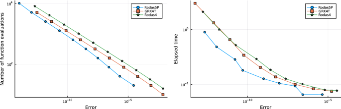

  

  Comparison of results of Rodas5P and modified methods GRK4T and Rodas4 for parabolic problem. Computations left with constant and right with adaptive stepsizes

  Table 8 Numerical results (error and order) for problem 4 (Index-2 DAE)

  Table 9 Numerical results (error) for dense output formulae

  Fig. 4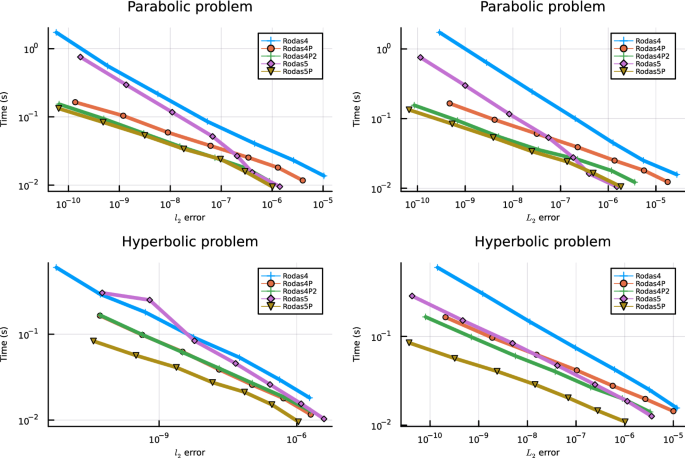

  

  Work-precision diagrams for parabolic and hyperbolic problems

  Fig. 5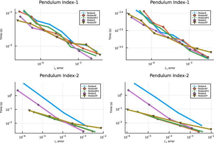

  

  Work-precision diagrams for the pendulum problem in index-1 and index-2 formulation

  Fig. 6

  

  Work-precision diagrams for two transistor amplifier and water tube problem

  Fig. 7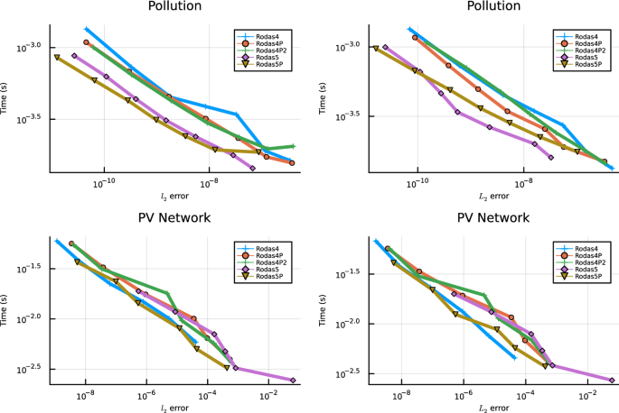

  

  Work-precision diagrams for pollution problem and photovoltaic network

  The third equation describes the consumer that demands a power P(t). It is assumed that P(t) represents a constant power, but it is switched on or off every hour. The discontinuities occurring in the process are, however, suitably smoothed. The fourth equation models the voltage-current characteristics of the PV element with given constants $c_i$, $i=1,..,6$. The battery is described by equations five to seven. Here, $R_0$, $R_1$, C are internal ohmic resistors and an internal capacity, respectively. The open-circuit voltage $u_0$ is described by a third-degree polynomial depending on the charge $q_B$. The main difficulties in this example are the solution of the nonlinear characteristics of the PV element and the switching processes of the load. The complete Julia Implementation is listed in the Appendix. Figure 7 shows that in this example the methods |Rodas4| and |Rodas5P| are most suitable.

5 Conclusion

Based on the construction method for |Rodas4P2| a new set of coefficients for |Rodas5| could be derived. The new |Rodas5P| method combines the properties of |Rodas5| (high order for standard problems) and |Rodas4P| or |Rodas4P2| (low order reduction for Prothero-Robinson model and parabolic problems). Moreover, it was possible to compute a fourth-order dense output formula for both methods, |Rodas5| and |Rodas5P|.

In all model problems the numerical results of the new method are in the range of the best methods from the class of Rodas schemes studied.

Therefore, |Rodas5P| can be recommended in the future as a standard method for stiff problems and index-1 DAEs for medium to high accuracy requirements within the Julia package |DifferentialEquations.jl|.

A Appendix

Work-precision diagrams for photovoltaic network with Julia

References

Alonso-Mallo, I., Cano, B.: Spectral/Rosenbrock discretizations without order reduction for linear parabolic problems. APNUM 41(2), 247–268 (2002)
Alonso-Mallo, I., Cano, B.: Efficient time integration of nonlinear partial differential equations by means of Rosenbrock methods. Mathematics 9(16), 1970 (2021). https://doi.org/10.3390/math9161970
Di Marzo, G.: RODAS5(4)-Méthodes de Rosenbrock d’ordre 5(4) adaptées aux problemes différentiels-algébriques. MSc mathematics thesis, Faculty of Science, University of Geneva, Switzerland (1993)
Hairer, E., Wanner, G.: Solving Ordinary Differential Equations II, Stiff and Differential Algebraic Problems, 2nd edn. Springer-Verlag, Berlin Heidelberg (1996)
Jax, T.: A rooted-tree based derivation of ROW-type methods with arbitrary Jacobian entries for solving index-one DAEs, Dissertation, University Wuppertal (2019)
Kaps, P., Rentrop, P.: Generalized Runge–Kutta methods of order four with stepsize control for stiff ordinary differential equations. Numer. Math. 33, 55–68 (1979)
Lamour, R., März, R., Tischendorf, C.: Differential-Algebraic Equations: A Projector Based Analysis, Differential-Algebraic Equations Forum book series. Springer, London (2013)
Lang, J.: Rosenbrock–Wanner Methods: Construction and Mission. In: Jax, T., Bartel, A., Ehrhardt, M., Günther, M., Steinebach, G. (eds.) Rosenbrock–Wanner-Type Methods, pp. 1–17. Mathematics Online First Collections Springer, Cham (2021). https://doi.org/10.1007/978-3-030-76810-2_2
Lang, J., Teleaga, D.: Towards a fully space-time adaptive FEM for magnetoquasistatics. IEEE Trans. Magn. 44, 1238–1241 (2008)
Lang, J., Verwer, J.G.: ROS3P-An Accurate Third-Order Rosenbrock Solver Designed for Parabolic Problems. J. BIT Numer. Math. 41, 731 (2001). https://doi.org/10.1023/A:1021900219772
Lubich, Ch., Roche, M.: Rosenbrock methods for differential-algebraic systems with solution-dependent singular matrix multiplying the derivative. Computing 43, 325–342 (1990). https://doi.org/10.1007/BF02241653
Mazzia, F., Cash, J.R., Soetaert, K.: A test set for stiff initial value problem solvers in the open source software R. J. Comput. Appl. Math. 236, 4119–4131 (2012)
Mazzia, F., Magherini, C.: Test set for initial value problem solvers, release 2.4 (Rep. 4/2008). Department of Mathematics, University of Bari, Italy. see https://archimede.uniba.it/testset/testsetivpsolvers/
Ostermann, A., Roche, M.: Rosenbrock methods for partial differential equations and fractional orders of convergence. SIAM J. Numer. Anal. 30, 1084–1098 (1993)
Prothero, A., Robinson, A.: The stability and accuracy of one-step methods. Math. Comp. 28, 145–162 (1974)
Rackauckas, C., Nie, Q.: Differentialequations.jl-a performant and feature-rich ecosystem for solving differential equations in Julia. J. Open Res. Softw. 5(1), 15 (2017)
Rang, J.: Improved traditional Rosenbrock–Wanner methods for stiff ODEs and DAEs. J. Comput. Appl. Math. 286, 128–144 (2015)
Rang, J.: The Prothero and Robinson example: Convergence studies for Runge–Kutta and Rosenbrock–Wanner methods. Appl. Numer. Math. 108, 37–56 (2016)
Rentrop, P., Roche, M., Steinebach, G.: The application of Rosenbrock–Wanner type methods with stepsize control in differential-algebraic equations. Numer. Math. 55, 545–563 (1989)
Roche, M.: Rosenbrock methods for differential algebraic equations. Numer. Math. 52, 45–63 (1988)
Sandu, A., Verwer, J.G., Van Loon, M., Carmichael, G.R., Potra, F.A., Dabdub, D., Seinfeld, J.H.: Benchmarking stiff ode solvers for atmospheric chemistry problems-I. implicit vs explicit. Atmos. Environ. 31(19), 3151–3166 (1997). https://doi.org/10.1016/S1352-2310(97)00059-9
Sanz-Serna, J.M., Verwer, J.G., Hundsdorfer, W.H.: Convergence and order reduction of Runge–Kutta schemes applied to evolutionary problems in partial differential eqautions. Numer. Math. 50, 405–418 (1986)
Scholz, S.: Order barriers for the B-convergence of ROW methods. Computing 41, 219–235 (1989)
Steinebach, G.: Order-reduction of ROW-methods for DAEs and method of lines applications. Preprint-Nr. 1741, FB Mathematik, TH Darmstadt (1995)
Steinebach, G.: Improvement of Rosenbrock–Wanner Method RODASP. In: Reis, T., Grundel, S., Schöps, S. (eds.) Progress in differential-algebraic equations II. Differential-algebraic equations forum, pp. 165–184. Springer, Cham (2020). https://doi.org/10.1007/978-3-030-53905-4_6
Steinebach, G., Dreistadt, D.M.: Water and hydrogen flow in networks: modelling and numerical solution by ROW methods. In: Jax, T., Bartel, A., Ehrhardt, M., Günther, M., Steinebach, G. (eds.) Rosenbrock–Wanner-Type Methods, pp. 19–47. Mathematics Online First Collections, Springer, Cham (2021)
Verwer, J.G.: Gauss-Seidel iteration for stiff ODEs from chemical kinetics. SIAM J. Sci. Comput. 15(5), 1243–1259 (1994)
Acknowledgements
This article is dedicated to my professor Peter Rentrop, who introduced me to the world of Rosenbrock–Wanner methods in 1986. Sincere thanks to Christopher Rackauckas for supporting me during implementation of the method in DifferentialEquations.jl and to the two reviewers for valuable comments to improve the paper.
Funding
Open Access funding enabled and organized by Projekt DEAL.
Author information
Authors and Affiliations
Corresponding author
Ethics declarations
Conflict of interest
The author declare that they have no conflict of interest.
Additional information
Publisher's Note
Springer Nature remains neutral with regard to jurisdictional claims in published maps and institutional affiliations.
Handling Editor: Antonella Zanna Munthe-Kaas.