On the interplay between cosmological shock waves and their environment

Abstract

Cosmological shock waves are tracers of the thermal history of the structures in the Universe. They play a crucial role in redistributing the energy within the cosmic structures and are also amongst the main ingredients of galaxy and galaxy cluster formation. Understanding this important function requires a proper description of the interplay between shocks and the different environments where they can be found. In this paper, an Adaptive Mesh Refinement (AMR) Eulerian cosmological simulation is analysed by means of a shock-finding algorithm that allows to generate shock wave maps. Based on the population of dark matter halos and on the distribution of density contrast in the simulation, we classify the shocks in five different environments. These range from galaxy clusters to voids. The shock distribution function and the shocks power spectrum are studied for these environments dynamics. We find that shock waves on different environments undergo different formation and evolution processes, showing as well different characteristics. We identify three different phases of formation, evolution and dissipation of these shock waves, and an intricate migration between distinct environments and scales. Shock waves initially form at external, low density regions and are merged and amplified through the collapse of structures. Shock waves and cosmic structures follow a parallel evolution. Later on, shocks start to detach from them and dissipate. We also find that most of the power that shock waves dissipate is found at scales of $k \sim0.5~\mbox{Mpc}^{-1}$, with a secondary peak at $k \sim8~\mbox{Mpc}^{-1}$. The evolution of the shocks power spectrum confirms that shock waves evolution is coupled and conditioned by their environment.

1 Introduction

The gas gravitational accretion gradually builds the elements found within our Universe following a bottom-up pattern (White and Frenk 1991). The resulting Large-Scale Structure (LSS) is comprised by various elements that hugely vary in size, from the small dwarf galaxies up to the cosmic web (see Kravtsov and Borgani 2012; Planelles et al. 2015, for recent reviews and references therein).

As gas infalls into the growing structures, they virialise and become pressure supported. During the accretion process, the sound speed at the borders of these regions decreases beneath the pace at which the baryonic material falls into them. This eventually generates accretion shock waves at the confines of the structures, since the thermal information regarding the presence of the material inside a region is not able to cross its outer boundaries. As a consequence, gravitational collapse continues. The thermalisation generated by the resulting shock front is a likely explanation for both the high temperatures reached within the intracluster medium (ICM; e.g. Quilis et al. 1998; Davé et al. 1999), and the radio emission detected at the peripheral regions of some galaxy clusters (see Ferrari et al. 2008; Feretti et al. 2012, and references therein, for recent reviews on extended radio emission from galaxy clusters).

Therefore, the physics of cosmological shock waves is crucial for a comprehensive understanding of the whole process of formation and evolution of cosmic structures in the Universe (e.g. Bykov et al. 2008; Dolag et al. 2008, for reviews). These shocks form altogether with cosmic structures, playing a crucial role in their evolution. The observational detection of shock waves is frequently connected with the observation of sharp jumps in some thermodynamical properties of the medium where the shock is located. Accretion shock waves have been elusive for direct observations, and no candidates have been discovered to date (see Brown et al. 2011, and references therein, for an analysis of different shock structures observed in a radio-selected galaxy cluster). The main difficulty to detect them is the low density of the medium where they are located, compared with the values within clusters or filaments. Therefore, X-ray emission generated at these outskirts, where stronger shocks are expected, is generally weak. Most cosmological shock detections occurred in radio ranges, as a diffusive shock acceleration process (DSA; Blandford and Ostriker 1978) is expected to produce electrons energetic enough to generate synchrotron emission (Ensslin et al. 1998; Giacintucci et al. 2008). These sources, known as radio relics, have been detected with relative ease (e.g. Ferrari et al. 2008; van Weeren et al. 2010; Brüggen et al. 2011; Feretti et al. 2012). Observations in X-rays or in the millimetre waveband through the Sunyaev-Zel’dovich effect (SZ effect; Sunyaev and Zeldovich 1972) have also confirmed that, within cosmological structures, shock waves mainly related to galaxy cluster dynamics can also be detected (e.g. Markevitch et al. 2002; Markevitch and Vikhlinin 2007; Ferrari et al. 2011; Botteon et al. 2016; Akamatsu et al. 2016).

A purely analytical approach to study cosmological shocks has been complicated to date, as the morphologies of the involved components are complex and intricate (Pavlidou and Fields 2005; Sheth and Tormen 1999). In this sense, numerical simulations represent the most self-consistent theoretical approach to study shock waves (e.g. Quilis et al. 1998; Miniati et al. 2000; Skillman et al. 2008; Vazza et al. 2009a; Araya-Melo et al. 2012; Planelles and Quilis 2013; Schaal and Springel 2015; Beck et al. 2016). Thanks to these numerical studies, now it is well established that shocks form around all the different structures of the Universe as an intricate network wrapping the LSS (Quilis et al. 1998; Miniati et al. 2000). Two main types of shock waves can be differentiated depending on their overall characteristics (Miniati et al. 2001; Ryu et al. 2003): external accretion shocks that surround the larger structures, and internal shocks, contained within the others and typically caused by the dynamics of elements such as galaxies or galaxy clusters.

Numerical simulations also indicate that shock waves with high Mach numbers¹ (typically $\mathcal{M} > 10$) correspond to accretion shocks that wrap the cosmic structures, fuelled by the flow of infalling cold gas. Among these accretion shocks, accretion shocks related to filaments generally involve lower Mach numbers ($10 < \mathcal{M} < 20$) than accretion shocks connected to galaxy clusters ($\mathcal {M} > 20$, e.g. Pfrommer et al. 2006; Skillman et al. 2008; Vazza et al. 2015a,b). Weaker shock waves can be associated to dissipation processes, with Mach numbers $4 < \mathcal{M} < 10$, or to merger events, reaching even lower Mach numbers ($\mathcal {M} \lesssim 1.5$; e.g. Gabici and Blasi 2003; Ryu et al. 2003; Battaglia et al. 2009; Skillman et al. 2010; Nuza et al. 2012; Araya-Melo et al. 2012).

Various significant phenomena are attributed to the existence of cosmological shock waves, such as the infalling gas thermalisation during accretion processes, which generates the baryonic pressure support, or the virialisation of halos through internal shocks. Several studies also indicate that DSA of cosmic rays (CRs) occurs in shock waves (Kang et al. 2007). Various authors have studied the expected spectrum of cosmic rays, suggesting that these particles contribute to the radio emission found in radio relics (e.g. Keshet et al. 2003; Vazza et al. 2009a; Hong et al. 2014, 2015; Wittor et al. 2017). Furthermore, recent observational findings suggest that cosmological shock waves resulting from galaxy cluster mergers may lead to star formation bursts in the internal galaxies (Stroe et al. 2015). Shock waves are also responsible of producing turbulence inside the ICM (e.g. Vazza et al. 2009b) or amplifying magnetic fields (e.g. Roettiger et al. 1999; see also Brüggen et al. 2011, Skillman et al. 2013, Vazza et al. 2015b, Wittor et al. 2016, 2017, for studies of shocks in magneto-hydrodynamic simulations). All these phenomena will affect the evolution of the cosmic structures, suggesting a complex interrelation between shocks and them.

Shock waves have also been suggested as an indirect method to measure the dark matter content of galaxy clusters (Planelles and Quilis 2013). Thus, shock waves are both ingredients and consequence of the diverse processes that progressively build up the cosmic structures, and their study allows us to recover an important amount of information regarding the formation and thermal history of the LSS. The relevance of cosmological shocks increases nowadays mainly due to the upcoming observational facilities like the Square-Kilometre Array² (SKA; e.g. Acosta-Pulido et al. 2015) that will be capable of, not just detecting a vast amount of diffuse radio sources, such as radio relics, but also study them in detail (e.g. Gaensler et al. 2004; Rawlings et al. 2004; Nuza et al. 2012; Kale et al. 2016). This will open a new window to look at the formation of the cosmic structures.

The aim of this paper is to perform a detailed description of the existing connection between cosmological shock waves and the different environments where they reside. In order to do so, an Adaptive Mesh Refinement (AMR) Eulerian cosmological simulation, accounting for radiative cooling and star formation, has been performed with the MASCLET code (Quilis 2004). The outputs of this simulation have been analysed by means of two numerical tools: a shock-finding algorithm (Planelles and Quilis 2013), that allows us to identify and characterise the formation and evolution of shock waves, and a halo finder (ASOHF; Planelles and Quilis 2010), that provides us with the population of dark matter halos found within our computational volume. Based on the population of dark matter halos and the distribution of density contrast in the simulation, we classify the environment where shocks are found in five different regimes, ranging from galaxy clusters to voids. The shocks distribution function and their power spectrum at different epochs, allow us to analyse in detail the intricate connection between cosmological shock waves and the medium where they are found.

This paper is organised as follows. In Sect. 2 we describe the main properties of the numerical simulation to be analysed; Sects. 3 and 4 include, respectively, a brief description of the shock-finder algorithm and the criteria employed to classify the different environments where shocks are found. In Sect. 5 we show results on the spatial distribution and temporal evolution of shock waves, their associated power spectrum and how their properties depend on the different environments where they are located. In Appendix A we give a detailed description of the Fast Fourier Transform (FFT) method we employ in our analysis. Finally, we summarise and discuss our results in Sect. 6.

2 Simulation setup

We study a cosmological simulation generated with MASCLET (Quilis 2004) in a standard cosmological concordance model. MASCLET is an AMR-Eulerian code that couples an hydrodynamical treatment to model the gas component of the Universe with N-body techniques for dark matter. The shock-capturing properties of the hydro algorithm allow us to avoid numerical artefacts and lead to an accurate treatment of discontinuities. A $\varLambda$CDM cosmology was assumed, with $\varOmega_{m} = 0.25$ matter density parameter, $\varOmega_{b} = 0.045$ baryon density parameter and $\varOmega_{\varLambda}= \varLambda/ 3 H_{0} ^{2} = 0.75$ for the cosmological constant. These values are consistent with the WMAP results (Hinshaw et al. 2013). The reduced Hubble constant in our simulation is $h = 0.73$. The initial density fluctuations power spectrum is scale invariant with $n_{s} = 1$ and normalised assuming $\sigma_{8} = 0.8$.

A CDM transfer function (Eisenstein and Hu 1998) is used. We generated our initial conditions at redshift $z = 50$. The grid coarse level covers a comoving length of $64~\mbox{Mpc}$ in a grid of $N_{x} = 256$ cells for each side (yielding a box of total volume $V_{T} = 64^{3}~\mbox{Mpc}^{3}$). The Zel’Dovich approximation is used to estimate which regions will require higher resolution. We set a first level of refinement wherever it is required. Dark matter particles are distributed accordingly, with lighter particles at the first level of refinement and heavier at the coarse grid. The best mass resolution is $_{\mathrm{DM}} = 2.7 \times10^{8} M_{\odot}$, equivalent to have the coarse grid sampled with $512^{3}$ particles with the same mass.

During the evolution of the simulation, subsequent AMR levels are created taking a pseudo-lagrangian approach. Thus, numerical cells having a baryonic (dark matter) mass larger than $1.04 \times10^{8} M _{\odot}$ ($4.74 \times10^{8} M_{\odot}$) are split in $2^{3}$ cubic cells, up to a maximum of $l = 6$ levels of resolution over the coarse grid. The highest spatial resolution in our simulation is $\Delta x \sim4~\mbox{kpc}$, considered an optimal value regarding the values tabulated in Vazza et al. (2011, see Table 1), where the authors study the resolution effects on the shock properties.

Our simulation includes cooling and heating processes: inverse Compton, free-free cooling and atomic and molecular cooling for primordial gases. UV heating background at $z \sim6$ is also considered (Haardt and Madau 1996).

Star formation processes and supernova (SN) feedback are also included in the simulation. We transform the cold gas inside a cell into star particles following the usual implementation $\dot{\rho}_{*} = \rho ^{1.5} / t_{0}^{*}$ (Kennicutt 1998), where $\rho_{*}$, $\rho$, and $t_{0}^{*}$ are the star density, gas density, and characteristic star formation time, respectively. Each SN explosion injects $10^{51}~\mbox{erg}$ of energy into the containing cell. No other feedback mechanisms are considered. The lack of an efficient central source of feedback, such as the one associated to central active galactic nuclei (AGN; e.g. Rasia et al. 2015), could generate unrealistic central temperature distributions in the innermost region ($<0.15R_{200}$) of our massive galaxy clusters. However, in the present analysis, where we focus on the large scale formation and evolution of cosmic shock waves, this shortcoming has negligible effects.

3 Shock-finding algorithm

Shock waves are detected during the post-processing phase using a shock-finding algorithm designed for MASCLET (see Planelles and Quilis 2013, for further details). Briefly, the shock finder associates shock waves with sharp jumps in various thermodynamic quantities. In this way, grid cells matching the expected conditions for the presence of a shock are identified and their corresponding Mach numbers are also computed. Two main methods for shock waves detection exist: those based on the temperature jump and those others based on the jump in velocity (e.g. Vazza et al. 2009a). Our shock-finding algorithm combines both methods to discriminate the shocked cells, whereas the associated Mach numbers are computed through the temperature jumps.

The discontinuities are examined using the Rankine-Hugoniot set of equations, which can be arranged to display a clear dependence on the Mach number:

$$\begin{aligned} &\frac{\rho_{d}}{\rho_{u}} = 4 \cdot\frac{\mathcal{M}^{2}}{ \mathcal{M}^{2}+3}, \end{aligned}$$

(1)

$$\begin{aligned} &\frac{T_{d}}{T_{u}} = \frac{(\mathcal{M}^{2}-1)(\mathcal{M}^{2}+3)}{16 \mathcal{M}^{2}}, \end{aligned}$$

(2)

$$\begin{aligned} &\frac{S_{d}}{S_{u}} = \frac{(\mathcal{M}^{2}-1)(\mathcal{M}^{2}+3)}{16 \mathcal{M}^{2}} \biggl( \frac{\mathcal{M}^{2}+3}{4\mathcal{M}^{2}} \biggr) ^{2/3}, \end{aligned}$$

(3)

being $T$ the gas temperature and $S$ the gas pseudo-entropy ($S = T \cdot\rho^{1-\gamma}$) of the upstream ($X_{u}$) and downstream ($X _{d}$) mediums. An ideal gas equation of state $p = \rho R T / \mu$ and an adiabatic coefficient $\gamma= 5/3$ are assumed, being $p$, $R$ and $\mu$ the pressure of the gas, the ideal gas constant and the mean molecular weight, respectively. The relation between the unshocked (upstream) and shocked (downstream) mediums of a shock wave directly depends on the shock strength, characterised by its Mach number. As indicated by Eq. (1), the discontinuity in density is limited to a maximum of $\rho_{d} / \rho_{u} = 4$. Both the temperature and the velocity methods avoid studying density jumps to circumvent this noisy mechanism. Our algorithm focuses on compression and thermalisation effects. The algorithm, displayed step by step in Fig. 1, operates as follows:

• 1. Tentative shocked cells in the simulation are detected and marked. Using the continuity equation,

  $$ \frac{\partial\rho}{\partial t} = - \frac{1}{a(t)} \vec{\nabla} \cdot\vec{v}, $$

  (4)

  (where $a (t)$ is the scale factor) and the fact that shock waves compress the flow, the first condition that a shocked cell must fulfil is to have a negative velocity divergence,

  $$ \vec{\nabla} \cdot\vec{v} < 0 $$

  (5)

  where $\vec{v}$ is the peculiar velocity of the fluid within each cell. Cells meeting this condition are marked as tentatively shocked (panel a in Fig. 1).

  Fig. 1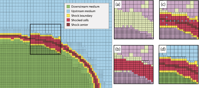

  

  Left panel: Sketch of a shock wave in an AMR grid detected using the shock-finding algorithm. Different colours stand for the different types of cells encountered during the process. The thickness of the shock wave has been exaggerated in the squared region for the sake of clarity. Usual thickness is of $\sim2\mbox{--}3$ cells. Right panels: Zoom-in of the black region displaying the shock identification process step by step. (a) Compression detection phase; temptatively shocked cells are marked in light yellow. (b) Shock thermalisation detection phase. (c) Boundaries recognition phase; from the cell that maximises the compression condition (star), we move along the spatial directions as indicated by the arrows. (d) Mach number characterisation phase

• 2. Shock waves differ from other compression mechanisms by a step jump in temperature and entropy over a thin layer. For the tentatively shocked cells identified by the previous condition, the temperature and entropy gradients are calculated. Cells displaying an increase in temperature and entropy in a given shock direction

  $$ (\vec{\nabla T}) \cdot(\vec{\nabla S}) > 0 $$

  (6)

  are marked as shocked cells (panel b in Fig. 1).

• 3. Once all shocked cells are identified, we focus on the cell that minimises $\vec{\nabla} \cdot\vec{v}$. Starting from this cell, the three spatial directions ($\mathrm{x},\mathrm{y},\mathrm{z}$) are evaluated forward and backward until one of the following conditions is not met:

  $$\begin{aligned} &T_{d} > T_{u}, \end{aligned}$$

  (7)
  $$\begin{aligned} &\rho_{d} > \rho_{u}, \end{aligned}$$

  (8)
  $$\begin{aligned} &v_{\mathrm{shock}} \neq0, \end{aligned}$$

  (9)

  or once a non-shocked cell is encountered. In this manner, the spatial extension of the shock is obtained. The process is recursively repeated on the remaining shock cells (panel c in Fig. 1).

• 4. We compute the Mach number at each shock retrieving the temperature of the upstream and downstream mediums and using Eq. (2). The Mach number is computed along each of the directions and combined as $\mathcal{M}^{2} = \mathcal{M}^{2} _{x} + \mathcal{M}^{2}_{y} + \mathcal{M}^{2}_{z}$ (panel d in Fig. 1).

A low Mach number threshold of $\mathcal{M}_{\mathrm{th}} = 1.3$ is assumed (e.g. Ryu et al. 2003; Skillman et al. 2008; Vazza et al. 2009a; Schaal and Springel 2015). The estimation of the final Mach number as described in the last item and the Mach number threshold imposed, avoid the overprediction, in a coordinate-split detection method as the one employed, of transonic and weakly supersonic regimes within the internal regions of clusters due to complex flow motions (e.g. Skillman et al. 2008; Vazza et al. 2009a).

We also note that the presence of radiative cooling might lead to spurious detections of shocks in the interstellar medium (e.g. Schaal et al. 2016). This requires very high resolutions, way over the ones captured in the present simulation and would have a main effect at very small scale regions.

4 Environmental classification

As indicated by observational and numerical studies, the properties of shock waves will be mainly determined by the nature of the event generating them (e.g., galactic dynamics, major cluster mergers, etc.) and the properties of the medium where they are located. Indeed, the two main factors influencing their evolution are the density and the temperature of this environment. To establish and study the relation between shock waves and their ambient, we present in this section the criteria employed to classify our numerical domain in five different regimes.

The shock-finding scheme gathers the densities and temperatures at the outer boundaries of the shocks. Since we estimate the shock Mach numbers through the jump in gas temperature, we base our environmental classification on the gas mass distribution of the simulation. In this way we guarantee an independent environmental classification with respect to the presence of shock waves. Additionally, density gradients generated by shock waves are smaller than the corresponding temperature gradients.

Therefore, based on the gas density, we broadly classify the environment into five different regimes: galaxy clusters, cluster outskirts, filaments, filament outskirts and voids. To more physically motivate the environments corresponding to galaxy clusters and cluster outskirts, we make use of the halo finder ASOHF (see Planelles and Quilis 2010; Knebe et al. 2011, for further details on the algorithm and its performance). This code provides us with a complete catalogue of dark matter halos at every redshift of the simulation. We consider a sample of 44 halos with masses $M_{200} \ge1.0\times10^{13}M_{\odot}$. For each halo we take as a reference the value of $R_{200}$, which corresponds to the radius enclosing a spherical region, centred at the position of the halo, with a mean density equal to 200 times the critical density of the Universe.

Once the halo catalogue is built, we proceed to classify the environment where the different shocked cells are embedded in the following way. Shocked cells contained within $R_{200}$ from the centre of any dark matter halo are classified as shocks in galaxy clusters, whereas those contained in a shell within a distance from the halo centre of $2 \ge r/R_{200} \ge1$ are classified in cluster outskirts. Note that, given the low-mass end of the employed halo catalogue, dark matter halos in our sample represent a wide range of masses, from galactic halos up to the largest galaxy clusters. Therefore, the environmental classification in galaxy clusters and cluster outskirts does not only represent the population of galaxy clusters (systems with, typically, $M_{200} \ge1.0\times10^{14}M_{\odot}$), but rather classifies the densest regions associated to cosmic structures. The shocks associated to the remaining shocked cells are classified attending exclusively to the gas density contrast of the upstream medium. Therefore, depending on the value of $\delta$ we divide the rest of the shock cells as shocks in filaments ($\delta> 3$), filament outskirts ($0.7< \delta< 3$) or voids ($0.1<\delta<0.7$). Other authors have employed environmental classifications based on similar density thresholds as Skillman et al. (2008), where they also employ temperature thresholds, or Vazza et al. (2009a). We include the additional environment filament outskirts, which allows to conservatively discriminate shocks found within filaments from those found in void regions.

Shock waves occurring in extremely low density environments, with a density contrast $\delta< 0.1$, are removed from the analysis. Due to the very low values that the ambient sound speed acquires at these very low densities, these shocks are in most cases numerical artefacts that display a highly noisy behaviour. As a consequence, most flows are considered shocked in these regions. The criteria employed in this environmental classification are summarised in Table 1.

Table 1 Environmental classification criteria. Our computational domain is classified in five different environments (namely, galaxy clusters, cluster outskirts, filaments, filament outskirts and voids) according to the density contrast, $\delta$, and the distance, $r$, of the considered shocked cell to the centre of any dark matter halo. For completeness, the last two columns show, at $z=0$, the ratio of the shocked volume for each environment $V_{\mathrm{sh}}$ with respect to the total shocked volume $V_{T, \mathrm{sh}}$, and the corresponding volume-weighted mean Mach number $\mathcal{M}_{m}$

An example of the resulting environmental classification is shown in the right panel of Fig. 2. For the sake of comparison, the left panel of Fig. 2 shows the corresponding gas density distribution at the same epoch. The defined galaxy cluster environment follows the galaxy cluster and groups seen in the overdensity distribution, whereas the outskirt environment is defined by the encompassing region, extending out to the interface with voids. The environment corresponding to the filaments captures the shocks contained within the filamentary structure, whereas the shocks in the external part of the filaments are classified as in filament outskirts. Finally, shocks that have escaped from the structures and are now contained in regions of very low density are classified as voids.

Fig. 2

Thin slices of gas density contrast $\delta_{\mathrm{gas}}$ (left panel) and environmental classification of the shocked cells (right panel) at redshift $z = 0$. The images are 32 Mpc side length and 32 kpc depth. See Table 1 for further details on the environmental classification performed

5 Results

In this Section, we describe the spatial and temporal evolution of the shock waves found in our simulation, their properties depending on the environment where they are found, and the characteristics of their power spectrum which is also compared with the gas matter power spectrum.

5.1 Distribution and evolution of shock waves

The distribution of shock waves over the Universe is directly coupled to the matter structures, as their growth is characterised by an intimate interplay. Consequently, the shock distribution mainly resembles the cosmic web of filaments and nodes over time, appearing the first shocks shortly after the first virialised structures form (e.g. Planelles and Quilis 2013).

In our simulation, the structure followed by shock fronts and their gaseous counterpart can be observed in Figs. 3 and 4, where thin slices of relevant physical quantities are displayed at different redshifts. In particular, whereas Fig. 3 shows the distribution of gas density contrast and gas temperature around the position of the biggest halo formed in our simulation at $z=0$, Fig. 4 shows the corresponding temporal evolution of the Mach number distribution, from $z=5$ down to $z=0$. Therefore, at $z=0$, the spatial distribution of shock waves and its connection with gas density and temperature can be obtained by comparing Fig. 3 with the top panel of Fig. 4. The inspection of these figures shows how the gas density contrast and the temperature drop separate the thermalised cosmic web from the void regions.

Fig. 3

Left and right panels show, respectively, a projection of the gas density contrast ($\delta_{\mathrm{gas}}$) and the gas temperature ($T_{\mathrm{gas}}$) at redshift $z = 0$. These images, centred at the position of the biggest halo found in our simulation, have $64~\mbox{Mpc}$ in side length and are integrated over $4~\mbox{Mpc}$ in depth

Fig. 4

Maps of the Mach number evolution from $z=5$ (bottom panel) to $z=0$ (top panel). The size of the images is the same as in Fig. 3

As shown in the top panel of Fig. 4, the extension of thermalised regions perfectly correlates with the position of external, high-Mach number shock waves wrapping the LSS. These shocks are typically resolved with cells of $\Delta x \sim 30~\mbox{kpc}$. Note that, as the quantities are integrated in depth and the shocks are thin surfaces, the Mach number seen in these projections is reduced by the inclusion of non-shocked regions in the line of sight.

From the distribution of shock waves at $z=0$, it is clear that higher Mach numbers are found at the largest scales. These external shock waves, with Mach numbers up to $\mathcal{M} \lesssim100$, expand towards the empty regions when the outer pressure decreases, maintaining a roughly constant flux of infalling gas and progressively escaping from their progenitor structures.

On the contrary, and in agreement with previous studies (e.g. Pavlidou and Fields 2005; Skillman et al. 2008), internal shocks have lower Mach numbers. These shock waves are consistent with being the by-product of small dark matter halos mergers and baryonic gas flows. Halos form at high redshifts and are progressively embedded inside bigger ones as the evolution approaches $z = 0$. In the inner regions, the high values reached by the density considerably increase the gas sound speed, which generates lower Mach numbers. Several authors have studied the dissipation of gravitational energy at shock waves (e.g. Vazza et al. 2009b; Skillman et al. 2013; Schaal and Springel 2015), indicating that, despite having low Mach numbers, the internal discontinuities are precisely the main sources of gravitational energy dissipation in their simulations.

The distribution of shock waves at any stage of the cosmic evolution is directly connected with the complex process of formation and evolution of cosmic structures. Figure 4 shows, for a thin slice of our simulation, the shock waves evolution over time from $z=5$ down to $z=0$. At high redshifts (from $z\sim5$ down to $z\sim3$), even when the cosmic network of galaxies and clusters is still not fully formed, the first shock waves start to form tightly wrapping their progenitor structures. Already at $z\sim2$, strong shock waves become precise tracers of the potential wells associated with forming filaments and proto-clusters, anticipating the distribution of the LSS obtained at $z=0$.

Nevertheless, observational detection of these strong, high-redshift shock waves is difficult, as their dominant effect is the heating of the primordial gas. In a further analysis, Skillman et al. (2013) also showed that most of the radio emission occurs at internal shocks in the presence of strong magnetic fields.

For completeness, Fig. 5 shows the temporal evolution of the fraction of shocked volume in our simulation (top panel), together with its corresponding mean volume-weighted Mach number (bottom panel). The Figures display the different environments and the total distribution.

Fig. 5

Temporal evolution of the fraction of shocked volume (top panel) and mean volume-weighted Mach number (bottom panel) for the different environments identified in the simulation

In the evolution of the total distribution (orange, solid line in Fig. 5), the highest fraction of shocked volume occurs at hight redshift, close to $z \sim5$, when the reionisation of the simulation triggers an increase in thermal pressure in the proto-structures, and generates various very low Mach number shocks (Schaal et al. 2016). At this early epoch, the shocked volume reaches a fraction of $\sim30\%$ of the computational box, and steadily declines as the redshift decreases. Overdense regions commence to merge and form the first structures, allowing the shock waves in their outskirts to interact amongst them as they grow. As a consequence, the fraction of shocked volume in the simulation is reduced and the mean Mach number is boosted, while larger structure shocks begin to be formed. Shock waves progressively dissipate, and the weakest shocks disappear when their ambient is depleted of their nurturing gas. The total shocked volume reaches a value of $\sim15\%$ at redshift $z = 0$, in broad agreement with other studies (Ryu et al. 2003; Vazza et al. 2009a; Planelles and Quilis 2013).

The redshift evolution of the simulation mean Mach number behaves similarly to the fraction of shocked volume. At $z \sim4$, the formation of most shock waves is accompanied by a high value of the mean Mach number ($\mathcal{M}_{\mathrm{mean}} \sim6$). Afterwards, as shock waves dissipate, the mean ℳ progressively decreases, reaching a value of $\mathcal{M}_{\mathrm{mean}} \sim4$ at $z=0$.

5.2 Dependence on the environment

We now analyse the connection between the main shock properties and the environment where they reside. In this regard, the analysis of Fig. 5 for the different environmental regimes provides several interesting trends. Attending to the final mean Mach numbers and their evolutions, we can broadly distinguish two different behaviours: the one associated to shock waves found in the densest environments, that is, galaxy clusters and cluster outskirts, and another related with the less dense regimes, i.e., filaments, filament outskirts and voids.

Galaxy clusters and cluster outskirts start with the highest mean Mach numbers at $z=4$ and end up with the lowest values at $z=0$. Filaments, filament outskirts and voids display a more steady mean Mach value and end up in a higher mean Mach state. As it would be expected, galaxy clusters and cluster outskirts are the only environments increasing the amount of volume occupied by their shocked cells as the redshift decreases. Shocks inside these environments are due to mergers, complex gas dynamics and stellar feedback. The local effect of stellar feedback is likely to only affect shocks on the smallest scales. A similar behaviour is also shown by filaments, at least from $z = 4 \mbox{ to } 2$. Afterwards, the volume they occupy remains approximately constant.

To deepen in the study of the interplay between shock waves and the different environments, we employ the Shock Distribution Function (SDF; Planelles and Quilis 2013). Figure 6 shows, in log-log scale, the normalised number of cells within a determined Mach number interval as a function of the Mach number at $z=0, 1, \mbox{ and } 3$ for the total distribution of shocks cells and for the different environments in which they have been classified.

Fig. 6

Normalised distribution of shock Mach numbers as a function of the Mach number. The panels display, from top to bottom, results at $z = 0, 1 \mbox{ and } 3$, respectively. At each redshift, the total (orange line) and all the environments are considered

From $z\sim3$, when the LSS begins to be defined, the SDF of the total distribution of shocked cells displays two main trends corresponding to low and high Mach numbers. At higher redshifts, the gravitational collapse forms the first shock waves in the simulation with relatively low Mach numbers. We would like to note that the reionisation background behaves as a uniform heating field at high redshift ($z \sim7$), representing a source of reheating to model the subgrid formation of the first massive stars. This reionisation triggers the formation of very low Mach number shocks in low density regions, which are not expected to have a large impact at lower redshifts. On the other hand, this heats up void regions and, therefore, is expected to avoid unrealistically high Mach numbers for accretion shocks (see Vazza et al. 2009a, where the authors also study the impact on shocks of different reionisation implementations).

As the evolution proceeds, the accretion shocks consolidate and the potential wells generated by different cosmic structures become deeper.

When the evolution reaches $z\sim3$, the epoch of formation of strong accretion shock waves is finished and their SDF can be described by two different power-laws, $dN(\mathcal{M}) \propto\mathcal{M}^{\alpha}$, governing the low and high Mach number regimes. From this moment, even when the shock waves in the simulation expand and fade, the distribution maintains this structure down to redshift $z = 0$. The slope for the power-laws during this later epoch of expansion down to $z = 0$ are $\alpha_{\mathrm{low}\mbox{-}{\mathcal{M}}} \sim-1.5 \pm0.1$ for most of the shocks, and $\alpha_{\mathrm{high}\mbox{-}{\mathcal{M}}} \sim-4.5 \pm0.1$ for the suppressed, high-Mach number. The break of the double power-law or, in other words, the change between these two regimes, takes place at around $\mathcal{M}_{\mathrm{break}} \sim50$. The inclusion of AGN feedback is expected to contribute to increase the SDF at high Mach numbers (Vazza et al. 2013; Schaal et al. 2016). This type of feedback is expected to be non-negligible around $z = 2$ and it could contribute to form a more shallow power-law in the high Mach regime, especially in the densest environments studied.

Observing the distribution of shock waves over the different environments, initially, shocks form in the most external regions of the first potential wells. These shocks expand towards voids. Regions within these shocks will later become the densest regions in the LSS and, therefore, they will be associated to different environments.

This increase of gravitational potential and the coalescence of shocks will be responsible of displacing the shocks towards higher Mach numbers as the redshift decreases. Regardless of the particular stellar feedback prescription, gravity and gas dynamics are almost the exclusive drivers of shocks evolution in the absence of AGN feedback (e.g. Vazza et al. 2013; Schaal et al. 2016).

In general, although with a different normalisation, shocks in filaments, filament outskirts and voids show a similar SDF evolution than the total distribution of shocked cells, with voids being the dominant environment.

In addition, as it is displayed in Fig. 5, these low-density environments are also similar in terms of volume and mean Mach number.

On the contrary, clusters and their outskirts, selected following a physical criterion based on the existence of dark matter halos, follow a different distribution over the Mach number range. Already at $z = 3$, these environments display a power-law at low Mach numbers and a plateau at $10<\mathcal{M}<100$ with a growing amount of low Mach number shocks. The presence of high Mach shocks is related with the accretion into the most massive structures within the simulation. The shocked volume within galaxy clusters and cluster outskirts increases exponentially with decreasing z at the same pace, that is, $V_{\mathrm{sh}} (z) \propto e^{(-0.6 \pm0.1)\,z}$. The distribution continues increasing its volume over time up to redshift $z \sim1$ and, from this point, progressively transforms into a steeper power-law at $z = 0$, where the presence of low Mach numbers dominates, accordingly with Fig. 5.

5.3 Shock waves power spectrum

The power spectra of the fluctuations in thermodynamical properties of a fluid, such as density, temperature, velocity or entropy, provide valuable information and constraints on the different astrophysical processes at play (e.g. Gaspari and Churazov 2013; Gaspari et al. 2014, and references therein). In our case, a useful tool to characterise the main features of shock waves at different scales, as well as their variations within the different environments, could be the shock waves power spectrum, that is, the Fourier analysis of the associated Mach number maps.

In order to carry out this analysis, we compute the discrete Fourier transform of Mach number, $\mathcal{M}_{k}$, for the 3D maps that we have obtained with the shock-finding algorithm (see Appendix A for further technical details on the method). The power spectrum, $P_{\mathrm{sh}}$, and the dimensionless shocks power spectrum, $\mathcal{F}(k)$, are defined, respectively, as

$$\begin{aligned} &P_{\mathrm{sh}}(k)=|\mathcal{M}_{k}^{2}|, \end{aligned}$$

(10)

$$\begin{aligned} &\mathcal{F}(k)=\frac{|k^{3} P_{\mathrm{sh}}(k)|}{2 \pi^{2}}, \end{aligned}$$

(11)

where $\mathcal{M}_{k}$ is the complex Mach number transform at a characteristic scale $k$.

In a similar way, we also define the gas matter power spectrum as

$$ P_{m}(k)=|\delta_{k}^{2}|, $$

(12)

where $\delta_{k}$ corresponds to the complex gas density contrast transform at a characteristic scale $k$.

In our particular implementation, we focus on the Fourier analysis of the central $32~\mbox{Mpc}$ cubic box, which is the best numerically resolved. For this volume, the characteristic wavelengths range from a minimum value $k_{\mathrm{min}} \sim0.4~\mbox{Mpc}^{-1}$ up to a maximum of $k_{\mathrm{max}} \sim170~\mbox{Mpc}^{-1}$.

The study of the Mach number spectrum allows us to identify how gas thermalisation effects are distributed over different scales.

Figure 7 presents the dimensionless power spectrum of the Mach numbers at $z=0, 1, 3$ as a function of the spectral wavelength. This distribution is shown for the total sample of shocked cells (black solid lines) as well as for the different environmental classifications in which we have divided our shocks. To improve the clarity in the comparison, we have increased the power for the clusters and cluster outskirts lines by a factor 10.

Fig. 7

The dimensionless power spectrum of the shock waves, $\mathcal{F}(k)$ over the wavelength $k$ for redshifts $z = 0$, $z = 1$ and $z = 3$ respectively. The power assigned to the Clusters and Outskirts has been increased by a factor of 10 for the sake of clarity

The power spectrum for all the shock waves displays four different regions related with the different types of scales at which shock waves can be found in the simulation. At the smallest scales ($k > 100~\mbox{Mpc}^{-1}$), we expect shock waves related with galaxies and small scale dynamics; the medium scales, comprised by $30~\mbox{Mpc}^{-1} < k < 100~\mbox{Mpc}^{-1}$, are expected to be caused by complex flow dynamics; large scales, with $2~\mbox{Mpc}^{-1} < k < 30~\mbox{Mpc}^{-1}$, can be related with galaxy clusters and, finally, the largest scales, $k < 2~\mbox{Mpc}^{-1}$, are attributed to the LSS. The dimensionless power spectrum of this distribution also displays two clear drops of power at $k \sim50~\mbox{Mpc}^{-1}$ and $k \sim100~\mbox{Mpc}^{-1}$, which are related with the change in the grid resolution, from the coarse to the first level of refinement and from the first to the second level, respectively.

Indeed, as shown in Gaspari and Churazov (2013), this effect in the Fourier spectrum is partially due to the numerical noise when reaching the non-periodic boundaries of a given level of resolution.

In the overall simulation, the small scale shock waves (large values of $k$) lose importance in comparison with the rest of scales. The analysis of the small scales has to be taken with care, due to possible resolution effects and the proximity to the Nyquist frequency. Only at the scale of galaxy clusters ($2~\mbox{Mpc}^{-1} < k < 30~\mbox{Mpc}^{-1}$) there is a noticeable change from $z = 3$ to $z = 0$. Namely, the temporal evolution of cluster scales is characterised by the formation of a bump, clearly visible at $z \sim3$ for $k \sim6~\mbox{Mpc}^{-1}$, and by a later displacement of the power towards lower k values that diminishes this feature. The power of the entire distribution decays rapidly from redshift $z = 3$ to $z = 1$. After this point, the decay is halted and the changes are found exclusively within the different environments. On the overall spectrum, most of the compressional effect of shock waves occurs typically on these scales. This can be expected from the important influence of the presence of strong accretion shock waves.

Unfolding the dimensionless power spectrum in the environments of our simulation displays information about their interplay with the shock waves. A clear differentiated behaviour is found again between the two cluster-related environments and the other distributions. In general, shocks expanding towards voids, filaments and filament outskirts broadly resemble the total distribution. Their associated power spectra can also be roughly described by the same four scales introduced above.

Most of the shock waves are generated in the interface between the voids and the other structures, specially at scales of $k \sim5\mbox{--}10~\mbox{Mpc}^{-1}$, comparable to the size of collapsing scales. As in the case of the total distribution, at these scales, a bump is formed at $z =3$ and progressively fades. As the redshift decreases to $z \sim1$, these shocks, and their forming collapsing regions, merge and are later identified inside other environments. This is reflected in the spectrum by a loss of power at the mentioned scale. As a consequence, the distribution flattens and becomes of the order of magnitude of the shocks in filament outskirts, which remains mostly unchanged. This phase of formation of shocks and migration towards other ambients is followed by the subsequent expansion of these shocks. This will dictate an eventual escape, back to the voids regions. At scales of $k < 2~\mbox{Mpc}^{-1}$, power is also lost from this voids environment, due to the formation of a background of shocks of transonic Mach numbers.

Shocks classified in filament outskirts display a stable spectrum, undergoing an increase of power from redshift $z \sim3$ to $z \sim1$ at scales $k < 5~\mbox{Mpc}^{-1}$. From $z = 1$, during the process of expansion, shock waves found within other environments will be transferred to the filament outskirts, producing a high power in the explained range from this moment onwards. After this point of $z = 1$, both the voids and the filament outskirts distribution display very similar trends, which is attributed to both regions representing the major contribution to gas compression occurring in the most external regions of the LSS.

Although filaments display a similar behaviour to their outskirts and the voids, their distribution is flatter and most of their power concentrates at $k < 1~\mbox{Mpc}^{-1}$. They undergo a subtle migration of power towards lower values of $k$. This is believed to be a consequence of the growth in size of the structures comprising this environment. That causes the distribution to become remarkably flat at $z \sim1$. After this moment, the environment starts to lose power, as the shock waves within this region dissipate.

Finally, the two environments related with clusters, i.e. galaxy clusters and cluster outskirts, follow a different power spectrum. At $z=3$ they concentrate all their power at scales $k > 10~\mbox{Mpc} ^{-1}$, being highly suppressed at other scales. At this high redshift, for $k > 10~\mbox{Mpc}^{-1}$, they also display flat spectra.

The growth of galaxy clusters triggers the appearance of strong accretion shock waves at scales similar to the size of the clusters, $k \sim10~\mbox{Mpc}^{-1}$, boosting the correlation towards $z = 1$. A similar boost is seen in cluster outskirts for smaller values of $k$. As the epoch of shock formation in this environment finishes, the simulation evolves to redshift $z = 0$. Shock waves start to expand and this translates into the cluster environment losing power at $k \sim5 {-} 10~\mbox{Mpc}^{-1}$. The distribution becomes flat again. Meanwhile, likely due to the spatial growth of galaxy clusters, the power grows at scales $k < 5~\mbox{Mpc}^{-1}$. At the same scales, shock waves in cluster outskirts also gain power by the migration of strong accretion shock waves escaping from galaxy clusters and the growth of their associated volume. These two environments also exhibit the highest relative ratio at scales $k > 100~\mbox{Mpc}^{-1}$, accordingly with the expected presence of internal dissipation shock waves, complex gas flows and galaxy dynamics. At $z = 0$, the cluster outskirts and the filaments distribution display a reasonably similar spectrum, with the most noticeable discrepancies being the higher power of the filaments at large scales and the large decay of power at the smallest scales of the filaments compared with the cluster outskirts. The first can be justified with the larger fraction of volume and extended nature of the filaments while the second is explained by the presence of more galaxies and high density regions within the cluster outskirts.

The presence of stellar feedback is expected to have little influence in the shocks power spectrum. However, AGN feedback is expected to affect the shocks power spectra. This feedback will trigger shocks at definite scales and might display as a pronounced bump in the studied spectra, with different effects due to different implementations (e.g. Vazza et al. 2013).

For the sake of comparison, Fig. 8 shows, at $z=0, 1, 3$, the dimensional shocks power spectrum, $P_{\mathrm{sh}}$, together with the gas matter power spectrum, $P_{m}$. Both power spectra have been normalised by requiring that their integral in the interval $[k_{\mathrm{min}},k_{\mathrm{max}}]$ to be equal to one. At $z=0$, the shocks power spectrum decays as a power-law, $P_{\mathrm{sh}}(k) = \vert \mathcal {M}_{k} \vert ^{2} \propto k^{\beta_{\mathrm{sh}}}$, with $\beta_{\mathrm{sh}} = -3.8 \pm0.1$. A similar shape is also found back to $z = 3$. The fact that this power-law is steeper than the slope found in the dimensional gas matter spectrum, which varies from $\beta_{m} = -1.6\pm0.1$ at $z=3$ down to $\beta_{m} = -3.0\pm0.1$ from $z=1$ to $z=0$, implies that there is more relative correlation at larger scales (lower values of $k$) for the case of the shock waves. A flat dimensionless power spectra in Fig. 7 implies also a $\beta= 3$. This is precisely found for the filaments environment from $z = 1$ onwards and the cluster outskirts for $z = 0$.

Fig. 8

Gas matter power spectrum ($P_{m}$; black line) and shocks power spectrum ($P_{\mathrm{sh}}$; red line) at $z = 0, 1, 3$ (from top to bottom panels, respectively) as defined in Eqs. (10)–(12)

In general, the shocks power spectrum is dominated by shocks in low density environments, in contrast to the gas matter power spectrum. The second yields more information about high density regions as galaxy clusters. The time evolution of both follow different patterns: while the gas matter spectrum peaks on structure scales and goes through a strong variation over redshift, the overall shocks power spectrum is characterised by dissipation and migration of shock waves between scales and environments. This is translated in a progressive lose of power and displacement of different features over decreasing redshift. It is also interesting to note that at $z=3$ the shocks power spectrum intersects the gas matter power spectrum at scales $k\sim15~\mbox{Mpc}^{-1}$, at $z=1$ both spectra are almost parallel, and they intersect each other again at $z=0$ but at larger scales ($k\sim0.7~\mbox{Mpc}^{-1}$).

Indeed, from $z=1$, both spectra are roughly parallel at the smallest scales. These results suggest that the shocks power spectrum evolves tightly coupled to the dynamical processes at scales $k>40\mbox{--}50~\mbox{Mpc}^{-1}$. From $z\sim3$, however, it decouples from the accretion processes, and the power starts to grow in larger scales while it is overall lost by dissipation.

Finally, Fig. 9 shows a comparison of the kinetic energy spectrum associated to the gas of the entire region and to the shock waves. In particular, the kinetic energy spectra associated to the whole domain are computed with the gas density and gas velocity fields of all the considered cells (dashed lines). On the other hand, the kinetic spectra associated to shock waves are computed by exclusively using the density in the shocked cells and the corresponding shock velocity components ($v_{\mathrm{shock}}$; continuous lines).

Fig. 9

Kinetic energy spectra of the central cubic box of the simulation at $z = 0, 1, 3$. The kinetic energy spectra associated to the shocked cells (calculated employing $v_{\mathrm{shock}}$; solid lines) and to the cells in the domain (dashed lines) are shown. Dot-dashed black line represents the Kolmogorov cascade, $\mathcal{E} _{\mathrm{kin}} \propto k^{-5/3}$, for reference

Shock waves seem to contain more kinetic energy at small scales ($k \gtrsim 3\mbox{--}4~\mbox{Mpc}^{-1}$) than at the rest of the domain. This trend is in line with the results presented in Skillman et al. (2008), where it was shown that low-Mach number shocks process a significant amount of kinetic energy. As redshift decreases, the amount of energy in shocks at the smallest scales is slightly reduced. This is consistent with shocks dissipating as thermalisation progresses at these small scales. A monotonic increase at large scales is also expected, due to the expansion of shock waves and the growth in size of galaxy clusters. The kinetic energy spectrum of the entire domain is broadly consistent with the characteristic Kolmogorov cascade towards the smallest scales, with a typical injection scale on the size of galaxy clusters. This injection scale becomes more evident as redshift decreases and clusters consolidate. However, the energy contained in shocks deviates from this turbulent cascade. Indeed, while on the largest scales both spectra are quite similar, once the injection scale of clusters is reached, the energy in shocks displays a flatter distribution. The fact that all scales contain similar orders of energy evidences that shocks are not the result of an energy cascade but they are rather generated by local gravitational phenomena. We find again that the spectrum conserves its shape as redshift decreases, indicating that shock waves structure remains approximately constant once they form. Due to the scaling with gas density, most of their energy is expected to be found within the densest regions. On the other hand, the shape of the spectra, deviating from the Kolmogorov cascade at the injection scale of clusters, allows a clear identification of this injection scale, on the order of $\sim5\mbox{--}10~\mbox{Mpc}$. The change of regime at the injection scale also favours most of the energy being held by internal shocks.

Cosmic shock waves are known to co-evolve with the LSS. Their spectra, with its main characteristics formed at high redshift, remains mostly unchanged by $z = 0$. This implies that shock waves contain thermal information about the high redshift universe. Furthermore, the study of their power spectrum reveals information on how different structures were spatially distributed at earlier times and how the primordial gas was thermalised to form the systems we observe today.

6 Summary

Cosmological shock waves are generated as a result of the formation, evolution and interaction of cosmic structures (e.g. Bykov et al. 2008, and references therein). As a consequence, they are present at all the relevant scales and are crucial processes to understand the energetics of the intergalactic medium.

Given the obvious connection between shock waves and cosmic structures, we have investigated in this paper the relation between shock waves and the cosmic environment where they reside. In particular, we have studied how the evolution of cosmic shock waves is affected by their ambients and their associated evolution. In addition, we analyse for the first time the power spectrum of shock waves. We identify different epochs in the formation of cosmological shock waves and their migration from their progenitor environments.

We have analysed the outputs of an AMR-Eulerian cosmological simulation, including radiative cooling and star formation, which has been carried out with the MASCLET code (Quilis 2004). A shock-finding algorithm (Planelles and Quilis 2013) has been employed in the post-processing phase to identify and characterise the formation and evolution of shock waves in the computational volume. Based on the population of dark matter halos and the density contrast distribution in the simulation, we have classified the environment where shocks are found in five different types, namely, galaxy clusters, cluster outskirts, filaments, filaments outskirts and voids. Despite its relative simplicity, this environmental classification, together with the shocks distribution function and their power spectrum, both studied at different epochs, has allowed us to analyse in detail the intricate connection between cosmological shock waves and the medium where they are found.

In our simulation, most shock waves are formed at redshifts between $z\sim5$ and $z\sim3$, in the external part of forming dark matter halos. From $z \sim3$ down to redshift $z \sim1$, these halos merge to progressively form the cosmic web. Meanwhile, the shocks coalesce, migrating towards denser environments. During this process, a double power-law distribution is formed in the Shock Distribution Function of the simulated universe, where Mach numbers over a given strength are strongly suppressed. As confirmed by the shocks power spectrum, the formation of shock waves around galaxy clusters becomes patent by the increase of power at scales $k \sim10~\mbox{Mpc}^{-1}$, which are populated by a high relative amount of high-Mach number shocks. Down to $z = 0$, the shock waves rapidly expand towards less dense environments, being dissipated in the process. At the present epoch, shock waves are specially important at scales of $k \sim0.5~\mbox{Mpc}^{-1}$ and shocked cells occupy a volume fraction of $\sim15\%$ with a mean Mach number of $\sim4$.

From the analysis of the connection between shock waves and environment, we confirm that shock waves are clear statistical tracers of the evolution of cosmological structures and their substructures, specially at scales larger than 200 kpc. Three main epochs are identified in the evolution of shock waves: an initial phase at very high redshift ($\sim z \in[5, 3]$) when the seeds of the shocks appear, an evolution phase at $z \in[3, 1]$ when the shocks seeds are transferred towards the defined environments and amplified. After a period of relative calm (approximately from $z\sim1$ down to $z\sim0.8$), an expansion phase when accretion shocks begin to escape to lower density environments and dissipate until $z=0$. Migration between the different environments and scales is identified, first from $k \sim2~\mbox{Mpc}^{-1}$ to $k \gtrsim5~\mbox{Mpc}^{-1}$, and then from $k \sim10~\mbox{Mpc}^{-1}$ towards larger scales. A progressive loss of power occurs for the shock waves at the present day, forecasting the future disappearance of cosmic accretion shocks (Cavaliere et al. 2011). Within denser regions, such as galaxy clusters and cluster outskirts, shock waves are described by different properties and spatial distributions. These shocks trigger the formation of the strongest shocks in the simulation but, at $z = 0$, they are mainly characterised by internal, low-Mach number shocks ($\mathcal{M} \sim1.5$).

At $z = 0$, both shocks within filaments and in cluster outskirts display a spectrum slope coincident with the gas matter spectrum.

It is interesting to remark that the power spectrum followed by the shock waves peaks at different scales than the density power spectrum, and is dominated by different environments, as galaxy clusters dominate the latter due to their high density compared to other structures.

Furthermore, shock waves seem to contain relatively more energy at cluster scales than the overall kinetic gas distribution. This is due to shock waves not being the result of a cascade of energy but being caused by local thermal and gravitational phenomena.

This result reinforces their crucial role in the process of structure formation and, at the same time, contributes to promote shocks as a promising probe to shed light on the nature of the different components of the Universe, not only at cluster scales but even at filamentary scales. Therefore, shock waves naturally arise as a window to the Universe, serving not only as a thermal record but also as structural tracers. The observation of cosmological shock waves will be a challenge for the future generation of radio telescopes, that will be able to exploit all the potentialities and physical implications that shock waves will bring to light. These observations will require to be guided and constrained, for which mock observations can be very useful. These wide surveys could potentially employ tools, such as the studied shocks power-spectrum, as new tests to study the structure of the Universe.

Future studies should also focus in the addition of cosmic rays models accelerated by shocks. This will require the inclusion of magnetic fields in the simulations. The effects of more detailed feedback implementations, specially for the case of stellar feedback, may alter dramatically the shock waves at galactic scales but it is unlikely to produce remarkable consequences on the cosmological shock structure.

Appendix A: FFT methods for the shocks distribution

To validate the employed Fast Fourier Transform (FFT) of the shock waves distribution, this Appendix illustrates the impact of different variations in the calculation procedure.

The negligible thickness of shock waves compared with the volume of the simulation implies that the FFT of this discontinuous distribution might display numerical artifacts. In particular, the presence of strong discrete signals surrounded by null values could act as flat window functions, which can lead to oscillations in Fourier space around the signal wavelength (Hewitt and Hewitt 1979).

The effect of local discreteness can be tested by introducing a local filter with a low spectral leakage. Figure 10 shows the effect of a local Gaussian filter in the region described in Sect. 5.3 at $z = 0$. Regardless of the $\sigma$ value employed in the Gaussian variance, there are no effects at scales $k < 10 \mbox{h Mpc}^{-1}$. At large scales, the effect of this discreteness disappears due to a more homogeneous appearance of the distribution. However, some effects can be seen at the smallest scales. As the local filter becomes wider, the resolution feature found at $k \sim100 \mbox{h Mpc}^{-1}$ disappears and power is lost. This change has to be interpreted with care, as increasing the thickness of the shock waves causes artificially thick shocks that are smoothed over AMR boundaries. Regarding artificial oscillations, none are found nor smoothed applying this filter. This indicates that the possible effect of the signal acting as a rectangular window is not influencing our results. Finally, the resolution of the box employed for the FFT is lower than the typical thickness of the smallest scale shocks in the simulation. Due to this, a value of $\sigma= 1$ unrealistically thickens them. The strength of the signal is also considerably reduced in the interphase between shocked and unshocked regions.

Fig. 10

FFT of the central cubic box of the simulation at $z = 0$. The $32~\mbox{Mpc}^{3}$ box is sampled with a uniform grid of $N$ cells. Left panel: Different lines display different values of $N$. In yellow we display the spectrum resulting of the zero-padded $N = 512$ box. The lines are shifted for the sake of clarity. Right panel: Different lines display the spectra after applying a local gaussian filter of width $\sigma$

As deduced from Fig. 10, the employed FFT is robust under different resolutions. As the resolution increases, the FFT probes even smaller frequencies. The oscillations leading to the Nyquist frequency are also displaced towards smaller scales. All the features far from the resolution limit are however conserved unaltered, resulting in the aforementioned robustness.

The calculation of the FFT employed in this paper assumes periodicity of the domain and isotropy of the shock waves in order to calculate the spectra as a combination of the three spatial dimensions.

As a different test, we also consider the effect of zero-padding to the studied box. This is a non-physical case, as the studied box is expected to exist within a larger region that fulfils the cosmological principle. In Fig. 10, the yellow line displays the effect of this zero-padding. This is computed by transferring the $N = 512$ box to the central [0.25–0.75] of a $N = 1024$ box. In this way, power is reduced at the largest scales due to the absence of correlation at the edges of the box after the zero-pad. This zero-pad is avoiding correlation to occur between periodic occurrences of the studied box.

The non-negligible effects of the AMR grid on the FFT analysis are discussed throughout the text (Sect. 5.3).

References

Acosta-Pulido, J.A., Agudo, I., Alberdi, A., Alcolea, J., Alfaro, E.J., Alonso-Herrero, A., Anglada, G., Arnalte-Mur, P., Ascasibar, Y., Ascaso, B., Azulay, R., Bachiller, R., Baez-Rubio, A., Battaner, E., Blasco, J., Brook, C.B., Bujarrabal, V., Busquet, G., Caballero-Garcia, M.D., Carrasco-Gonzalez, C., Casares, J., Castro-Tirado, A.J., Colina, L., Colomer, F., de Gregorio-Monsalvo, I., del Olmo, A., Desmurs, J.-F., Diego, J.M., Dominguez-Tenreiro, R., Estalella, R., Fernandez-Soto, A., Florido, E., Font, J., Font, J.A., Fuente, A., Garcia-Benito, R., Garcia-Burillo, S., Garcia-Lorenzo, B., Gil de Paz, A., Girart, J.M., Goicoechea, J.R., Gomez, J.F., Gonzalez-Garcia, M., Gonzalez-Martin, O., Gonzalez-Serrano, J.I., Gorgas, J., Gorosabel, J., Guijarro, A., Guirado, J.C., Hernandez-Garcia, L., Hernandez-Monteagudo, C., Herranz, D., Herrero-Illana, R., Hu, Y.-D., Huelamo, N., Huertas-Company, M., Iglesias-Paramo, J., Jeong, S., Jimenez-Serra, I., Knapen, J.H., Lineros, R.A., Lisenfeld, U., Marcaide, J.M., Marquez, I., Marti, J., Marti, J.M., Marti-Vidal, I., Martinez-Gonzalez, E., Martin-Pintado, J., Masegosa, J., Mayen-Gijon, J.M., Mezcua, M., Migliari, S., Mimica, P., Moldon, J., Morata, O., Negueruela, I., Oates, S.R., Osorio, M., Palau, A., Paredes, J.M., Perea, J., Perez-Gonzalez, P.G., Perez-Montero, E., Perez-Torres, M.A., Perucho, M., Planelles, S., Pons, J.A., Prieto, A., Quilis, V., Ramirez-Moreta, P., Ramos Almeida, C., Rea, N., Ribo, M., Rioja, M.J., Rodriguez Espinosa, J.M., Ros, E., Rubiño-Martin, J.A., Ruiz-Granados, B., Sabater, J., Sanchez, S., Sanchez-Contreras, C., Sanchez-Monge, A., Sanchez-Ramirez, R., Sintes, A.M., Solanes, J.M., Sopuerta, C.F., Tafalla, M., Tello, J.C., Tercero, B., Toribio, M.C., Torrelles, J.M., Torres, M.A.P., Usero, A., Verdes-Montenegro, L., Vidal-Garcia, A., Vielva, P., Vilchez, J., Zhang, B.-B.: arXiv e-prints 1506.03474 (2015)
Akamatsu, H., Gu, L., Shimwell, T.W., Mernier, F., Mao, J., Urdampilleta, I., de Plaa, J., Röttgering, H.J.A., Kaastra, J.S.: Astron. Astrophys. 593, 7 (2016). 1608.01669. doi:10.1051/0004-6361/201629275
Araya-Melo, P.A., Aragón-Calvo, M.A., Brüggen, M., Hoeft, M.: Mon. Not. R. Astron. Soc. 423, 2325 (2012). 1204.1759. doi:10.1111/j.1365-2966.2012.21042.x
Battaglia, N., Pfrommer, C., Sievers, J.L., Bond, J.R., Enßlin, T.A.: Mon. Not. R. Astron. Soc. 393, 1073 (2009). 0806.3272. doi:10.1111/j.1365-2966.2008.14136.x
Beck, A.M., Dolag, K., Donnert, J.M.F.: Mon. Not. R. Astron. Soc. 458, 2080 (2016). 1511.07444. doi:10.1093/mnras/stw487
Blandford, R.D., Ostriker, J.P.: Astrophys. J. Lett. 221, 29 (1978). doi:10.1086/182658
Botteon, A., Gastaldello, F., Brunetti, G., Kale, R.: Mon. Not. R. Astron. Soc. 463, 1534 (2016). 1607.04641. doi:10.1093/mnras/stw2089
Brown, S., Duesterhoeft, J., Rudnick, L.: Astrophys. J. Lett. 727, 25 (2011). 1011.4985. doi:10.1088/2041-8205/727/1/L25
Brüggen, M., van Weeren, R.J., Röttgering, H.J.A.: Mem. Soc. Astron. Ital. 82, 627 (2011). 1102.1926
Bykov, A.M., Dolag, K., Durret, F.: Space Sci. Rev. 134, 119 (2008). 0801.0995. doi:10.1007/s11214-008-9312-9
Cavaliere, A., Lapi, A., Fusco-Femiano, R.: Astron. Astrophys. 525, 110 (2011). 1010.4415. doi:10.1051/0004-6361/201015390
Davé, R., Hernquist, L., Katz, N., Weinberg, D.H.: Astrophys. J. 511, 521 (1999). astro-ph/9807177. doi:10.1086/306722
Dolag, K., Bykov, A.M., Diaferio, A.: Space Sci. Rev. 134, 311 (2008). 0801.1048. doi:10.1007/s11214-008-9319-2
Eisenstein, D.J., Hu, W.: Astrophys. J. 496, 605 (1998). astro-ph/9709112. doi:10.1086/305424
Ensslin, T.A., Biermann, P.L., Klein, U., Kohle, S.: Astron. Astrophys. 332, 395 (1998). astro-ph/9712293
Feretti, L., Giovannini, G., Govoni, F., Murgia, M.: Astron. Astrophys. Rev. 20, 54 (2012). 1205.1919. doi:10.1007/s00159-012-0054-z
Ferrari, C., Govoni, F., Schindler, S., Bykov, A.M., Rephaeli, Y.: Space Sci. Rev. 134, 93 (2008). 0801.0985. doi:10.1007/s11214-008-9311-x
Ferrari, C., Intema, H.T., Orrù, E., Govoni, F., Murgia, M., Mason, B., Bourdin, H., Asad, K.M., Mazzotta, P., Wise, M.W., Mroczkowski, T., Croston, J.H.: Astron. Astrophys. 534, 12 (2011). 1107.5945. doi:10.1051/0004-6361/201117788
Gabici, S., Blasi, P.: Astrophys. J. 583, 695 (2003). astro-ph/0207523. doi:10.1086/345429
Gaensler, B.M., Beck, R., Feretti, L.: New Astron. Rev. 48, 1003 (2004). astro-ph/0409100. doi:10.1016/j.newar.2004.09.003
Gaspari, M., Churazov, E.: Astron. Astrophys. 559, 78 (2013). 1307.4397. doi:10.1051/0004-6361/201322295
Gaspari, M., Churazov, E., Nagai, D., Lau, E.T., Zhuravleva, I.: Astron. Astrophys. 569, 67 (2014). 1404.5302. doi:10.1051/0004-6361/201424043
Giacintucci, S., Venturi, T., Macario, G., Dallacasa, D., Brunetti, G., Markevitch, M., Cassano, R., Bardelli, S., Athreya, R.: Astron. Astrophys. 486, 347 (2008). 0803.4127. doi:10.1051/0004-6361:200809459
Haardt, F., Madau, P.: Astrophys. J. 461, 20 (1996). astro-ph/9509093. doi:10.1086/177035
Hewitt, E., Hewitt, R.E.: Arch. Hist. Exact Sci. 21(2), 129 (1979). doi:10.1007/BF00330404
Hinshaw, G., Larson, D., Komatsu, E., Spergel, D.N., Bennett, C.L., Dunkley, J., Nolta, M.R., Halpern, M., Hill, R.S., Odegard, N., Page, L., Smith, K.M., Weiland, J.L., Gold, B., Jarosik, N., Kogut, A., Limon, M., Meyer, S.S., Tucker, G.S., Wollack, E., Wright, E.L.: Astrophys. J. Suppl. Ser. 208, 19 (2013). 1212.5226. doi:10.1088/0067-0049/208/2/19
Hong, S.E., Kang, H., Ryu, D.: Astrophys. J. 812, 49 (2015). 1504.03102. doi:10.1088/0004-637X/812/1/49
Hong, S.E., Ryu, D., Kang, H., Cen, R.: Astrophys. J. 785, 133 (2014). 1403.1420. doi:10.1088/0004-637X/785/2/133
Kale, R., Dwarakanath, K.S., Vir Lal, D., Bagchi, J., Paul, S., Malu, S., Datta, A., Parekh, V., Sharma, P., Pandey-Pommier, M.: J. Astrophys. Astron. 37, 31 (2016). 1610.08182. doi:10.1007/s12036-016-9406-9
Kang, H., Ryu, D., Cen, R., Ostriker, J.P.: Astrophys. J. 669, 729 (2007). 0704.1521. doi:10.1086/521717
Kennicutt, R.C. Jr.: Annu. Rev. Astron. Astrophys. 36, 189 (1998). astro-ph/9807187. doi:10.1146/annurev.astro.36.1.189
Keshet, U., Waxman, E., Loeb, A., Springel, V., Hernquist, L.: Astrophys. J. 585, 128 (2003). astro-ph/0202318. doi:10.1086/345946
Knebe, A., Knollmann, S.R., Muldrew, S.I., Pearce, F.R., Aragon-Calvo, M.A., Ascasibar, Y., Behroozi, P.S., Ceverino, D., Colombi, S., Diemand, J., Dolag, K., Falck, B.L., Fasel, P., Gardner, J., Gottlöber, S., Hsu, C.-H., Iannuzzi, F., Klypin, A., Lukić, Z., Maciejewski, M., McBride, C., Neyrinck, M.C., Planelles, S., Potter, D., Quilis, V., Rasera, Y., Read, J.I., Ricker, P.M., Roy, F., Springel, V., Stadel, J., Stinson, G., Sutter, P.M., Turchaninov, V., Tweed, D., Yepes, G., Zemp, M.: Mon. Not. R. Astron. Soc. 415, 2293 (2011). 1104.0949. doi:10.1111/j.1365-2966.2011.18858.x
Kravtsov, A.V., Borgani, S.: Annu. Rev. Astron. Astrophys. 50, 353 (2012). 1205.5556. doi:10.1146/annurev-astro-081811-125502
Markevitch, M., Vikhlinin, A.: Phys. Rep. 443, 1 (2007). astro-ph/0701821. doi:10.1016/j.physrep.2007.01.001
Markevitch, M., Gonzalez, A.H., David, L., Vikhlinin, A., Murray, S., Forman, W., Jones, C., Tucker, W.: Astrophys. J. Lett. 567, 27 (2002). astro-ph/0110468. doi:10.1086/339619
Miniati, F., Ryu, D., Kang, H., Jones, T.W., Cen, R., Ostriker, J.P.: Astrophys. J. 542, 608 (2000). astro-ph/0005444. doi:10.1086/317027
Miniati, F., Ryu, D., Kang, H., Jones, T.W.: Astrophys. J. 559, 59 (2001). astro-ph/0105465. doi:10.1086/322375
Nuza, S.E., Hoeft, M., van Weeren, R.J., Gottlöber, S., Yepes, G.: Mon. Not. R. Astron. Soc. 420, 2006 (2012). 1111.1721. doi:10.1111/j.1365-2966.2011.20118.x
Pavlidou, V., Fields, B.D.: Phys. Rev. D 71(4), 043510 (2005). astro-ph/0410338. doi:10.1103/PhysRevD.71.043510
Pfrommer, C., Springel, V., Enßlin, T.A., Jubelgas, M.: Mon. Not. R. Astron. Soc. 367, 113 (2006). astro-ph/0603483. doi:10.1111/j.1365-2966.2005.09953.x
Planelles, S., Quilis, V.: Astron. Astrophys. 519, 94 (2010). 1006.3205. doi:10.1051/0004-6361/201014214
Planelles, S., Quilis, V.: Mon. Not. R. Astron. Soc. 428, 1643 (2013). 1210.1369. doi:10.1093/mnras/sts142
Planelles, S., Schleicher, D.R.G., Bykov, A.M.: Space Sci. Rev. 188, 93 (2015). 1404.3956. doi:10.1007/s11214-014-0045-7
Quilis, V.: Mon. Not. R. Astron. Soc. 352, 1426 (2004). astro-ph/0405389. doi:10.1111/j.1365-2966.2004.08040.x
Quilis, V., Ibáñez, J.M., Sáez, D.: Astrophys. J. 502, 518 (1998). astro-ph/9803059. doi:10.1086/305932
Rasia, E., Borgani, S., Murante, G., Planelles, S., Beck, A.M., Biffi, V., Ragone-Figueroa, C., Granato, G.L., Steinborn, L.K., Dolag, K.: Astrophys. J. Lett. 813, 17 (2015). 1509.04247. doi:10.1088/2041-8205/813/1/L17
Rawlings, S., Abdalla, F.B., Bridle, S.L., Blake, C.A., Baugh, C.M., Greenhill, L.J., van der Hulst, J.M.: New Astron. Rev. 48, 1013 (2004). astro-ph/0409479. doi:10.1016/j.newar.2004.09.024
Roettiger, K., Stone, J.M., Burns, J.O.: Astrophys. J. 518, 594 (1999). astro-ph/9902105. doi:10.1086/307298
Ryu, D., Kang, H., Hallman, E., Jones, T.W.: Astrophys. J. 593, 599 (2003). astro-ph/0305164. doi:10.1086/376723
Schaal, K., Springel, V.: Mon. Not. R. Astron. Soc. 446, 3992 (2015). 1407.4117. doi:10.1093/mnras/stu2386
Schaal, K., Springel, V., Pakmor, R., Pfrommer, C., Nelson, D., Vogelsberger, M., Genel, S., Pillepich, A., Sijacki, D., Hernquist, L.: Mon. Not. R. Astron. Soc. 461, 4441 (2016). 1604.07401. doi:10.1093/mnras/stw1587
Sheth, R.K., Tormen, G.: Mon. Not. R. Astron. Soc. 308, 119 (1999). astro-ph/9901122. doi:10.1046/j.1365-8711.1999.02692.x
Skillman, S.W., O’Shea, B.W., Hallman, E.J., Burns, J.O., Norman, M.L.: Astrophys. J. 689, 1063 (2008). 0806.1522. doi:10.1086/592496
Skillman, S.W., Hallman, E.J., O’Shea, B.W., Burns, J.O.: In: American Astronomical Society Meeting Abstracts #215. Bulletin of the American Astronomical Society, vol. 42, p. 389 (2010)
Skillman, S.W., Xu, H., Hallman, E.J., O’Shea, B.W., Burns, J.O., Li, H., Collins, D.C., Norman, M.L.: Astrophys. J. 765, 21 (2013). 1211.3122. doi:10.1088/0004-637X/765/1/21
Stroe, A., Sobral, D., Dawson, W., Jee, M.J., Hoekstra, H., Wittman, D., van Weeren, R.J., Brüggen, M., Röttgering, H.J.A.: Mon. Not. R. Astron. Soc. 450, 646 (2015). 1410.2891. doi:10.1093/mnras/stu2519
Sunyaev, R.A., Zeldovich, Y.B.: Comments Astrophys. Space Phys. 4, 173 (1972)
van Weeren, R.J., Röttgering, H.J.A., Brüggen, M., Hoeft, M.: Science 330, 347 (2010). 1010.4306. doi:10.1126/science.1194293
Vazza, F., Brüggen, M., Gheller, C.: Mon. Not. R. Astron. Soc. 428, 2366 (2013). 1210.3541. doi:10.1093/mnras/sts213
Vazza, F., Brunetti, G., Gheller, C.: Mon. Not. R. Astron. Soc. 395, 1333 (2009a). 0808.0609. doi:10.1111/j.1365-2966.2009.14691.x
Vazza, F., Brunetti, G., Kritsuk, A., Wagner, R., Gheller, C., Norman, M.: Astron. Astrophys. 504, 33 (2009b). 0905.3169. doi:10.1051/0004-6361/200912535
Vazza, F., Dolag, K., Ryu, D., Brunetti, G., Gheller, C., Kang, H., Pfrommer, C.: Mon. Not. R. Astron. Soc. 418, 960 (2011). 1106.2159. doi:10.1111/j.1365-2966.2011.19546.x
Vazza, F., Eckert, D., Brüggen, M., Huber, B.: Mon. Not. R. Astron. Soc. 451, 2198 (2015a). 1505.02782. doi:10.1093/mnras/stv1072
Vazza, F., Ferrari, C., Brüggen, M., Bonafede, A., Gheller, C., Wang, P.: Astron. Astrophys. 580, 119 (2015b). 1503.08983. doi:10.1051/0004-6361/201526228
White, S.D.M., Frenk, C.S.: Astrophys. J. 379, 52 (1991). doi:10.1086/170483
Wittor, D., Vazza, F., Brüggen, M.: Galaxies 4, 71 (2016). 1612.04248. doi:10.3390/galaxies4040071
Wittor, D., Vazza, F., Brüggen, M.: Mon. Not. R. Astron. Soc. 464, 4448 (2017). 1610.05305. doi:10.1093/mnras/stw2631
Acknowledgements
The authors kindly thank the referee for a constructive criticism that helped to improve the quality of this manuscript. This work has been partially supported by the Spanish Ministerio de Economía y Competitividad (MINECO; grant AYA2013-48226-C-2-P and grant AYA2016-77237-C3-3-P) and Generalitat Valenciana (grant PROMETEO II/2014/069). SMA acknowledges a Iniciació a la Investigació scholarship from the Universitat de València and a Hintze scholarship from the Oxford Centre for Astrophysical Surveys which is funded through generous support from the Hintze Family Charitable Foundation. Simulations were carried at the Servei d’Informática de la Universitat de Valéncia using the Lluís Vives supercomputer. The authors also acknowledge the usage of the FFTW.
Author information
Authors and Affiliations
Corresponding author